On Quaternionic 3 CR-Structure and Pseudo-Riemannian Metric

Abstract

A CR-structure on a 2n +1-manifold gives a conformal class of Lorentz metrics on the Fefferman S1-bundle. This analogy is carried out to the quarternionic conformal 3-CR structure (a generalization of quaternionic CR- structure) on a 4n + 3 -manifold M. This structure produces a conformal class [g] of a pseudo-Riemannian metric g of type (4n + 3,3) on M × S3. Let (PSp(n +1,1), S4n+3) be the geometric model obtained from the projective boundary of the complete simply connected quaternionic hyperbolic manifold. We shall prove that M is locally modeled on (PSp(n +1,1), S4n+3) if and only if (M × S3 ,[g]) is conformally flat (i.e. the Weyl conformal curvature tensor vanishes).

Share and Cite:

Kamishima, Y. (2018) On Quaternionic 3 CR-Structure and Pseudo-Riemannian Metric. Applied Mathematics, 9, 114-129. doi: 10.4236/am.2018.92008.

1. Introduction

This paper concerns a geometric structure on ( 4 n + 3 ) -manifolds which is related with CR-structure and also quaternionic CR-structure (cf. [1] [2] ). Given a quaternionic CR-structure { ω α } α = 1 , 2 , 3 on a 4 n + 3 -manifold M, we have proved in [3] that the associated endomorphism J α on the 4n-bundle D naturally extends to a complex structure J ¯ α on ker   ω α . So we obtain 3 CR-structures on M. Taking into account this fact, we study the following geometric structure on ( 4 n + 3 ) -manifolds globally.

A hypercomplex 3 CR-structure on a ( 4 n + 3 ) -manifold M consists of (positive definite) 3 pseudo-Hermitian structures { ω α , J α } α = 1 , 2 , 3 on M which satisfies that

1) D = ∩ α = 1 3 ker   ω α is a 4n-dimensional subbundle of TM such that

D + [ D , D ] = T M .

2) Each J γ coincides with the endomorphism ( d ω β | D ) − 1 ∘ ( d ω α | D ) : D → D ( ( α , β , γ ) ~ ( 1,2,3 ) ) such that { J 1 , J 2 , J 3 } constitutes a hypercomplex structure on D .

We call the pair ( D , { J 1 , J 2 , J 3 } ) also a hypercomplex 3 CR-structure if it is represented by such pseudo-Hermitian structures on M. A quaternionic CR- structure is an example of our hypercomplex 3 CR-structure. As Sasakian 3- structure is equivalent with quaternionic CR-structure, Sasakian 3-structure is also an example. Especially the 4 n + 3 -dimensional standard sphere S 4 n + 3 is a hypercomplex 3 CR-manifold. The pair ( PSp ( n + 1,1 ) , S 4 n + 3 ) is the spherical homogeneous model of hypercomplex 3 CR-structure in the sense of Cartan geometry (cf. [4] ). First we study the properties of hypercomplex 3 CR-structure. Next we introduce a quaternionic 3 CR-structure on M in a local manner. In fact, let D be a 4n-dimensional subbundle endowed with a quaternionic structure Q on a ( 4 n + 3 ) -manifold M. The pair ( D , Q ) is called quaternionic 3 CR-structure if the following conditions hold:

1) D + [ D , D ] = T M ;

2) M has an open cover { U i } i ∈ Λ each U i of which admits a hypercomplex 3 CR-structure ( ω α ( i ) , J α ( i ) ) α = 1 , 2 , 3 such that:

a) D | U i = ∩ α = 1 3 ker ω α ( i ) ;

b) Each hypercomplex structure { J 1 ( i ) , J 2 ( i ) , J 3 ( i ) } i ∈ Λ on D | U i generates a quaternionic structure Q on D .

A 4 n + 3 -manifold equipped with this structure is said to be a quaternionic 3 CR-manifold. A typical example of a quaternionic 3 CR-manifold but not a hypercomplex 3 CR-manifold is a quaterninic Heisenberg nilmanifold. In this paper, we shall study an invariant for quaternionic 3 CR-structure on ( 4 n + 3 ) - manifolds.

Theorem A. Let ( M , { D , Q } ) be a quaternionic 3 CR-manifold. There exists a pseudo-Riemannian metric g of type ( 4 n + 3,3 ) on M × S 3 . Then the con- formal class [ g ] is an invariant for quaternionic 3 CR-structure.

As well as the spherical quaternionic 3 CR homogeneous manifold S 4 n + 3 , we have the pseudo-Riemannian homogeneous manifold S 4 n + 3 × S 3 which is a two-fold covering of the pseudo-Riemannian homogeneous manifold ( S 4 n + 3 × ℤ 2 S 3 , g 0 ) . The pair ( PSp ( n + 1,1 ) × SO ( 3 ) , S 4 n + 3 × ℤ 2 S 3 ) is a subgeometry of conformally flat pseudo-Riemannian homogeneous geometry ( PO ( 4 n + 4,4 ) , S 4 n + 3 × ℤ 2 S 3 ) where PSp ( n + 1,1 ) × SO ( 3 ) ≤ PO ( 4 n + 4,4 ) .

Theorem B. A quaternionic 3 CR-manifold M is spherical (i.e. locally modeled on ( PSp ( n + 1,1 ) , S 4 n + 3 ) ) if and only if the pseudo-Riemannian manifold ( M × S 3 , g ) is conformally flat, more precisely it is locally modeled on ( PSp ( n + 1,1 ) × SO ( 3 ) , S 4 n + 3 × ℤ 2 S 3 ) .

We have constructed a conformal invariant on ( 4 n + 3 ) -dimensional pseudo- conformal quaternionic CR manifolds in [3] . We think that the Weyl conformal curvature of our new pseudo-Riemannian metric obtained in Theorem A is theoretically the same as this invariant in view of Uniformization Theorem B. But we do not know whether they coincide.

Section 2 is a review of previous results and to give some definition of our notion. In Section 3 we prove the conformal equivalence of our pseudo-Riemannian metrics and prove Theorem A. In Section 4 first we relate our spherical 3 CR-homogeneous model ( PSp ( n + 1,1 ) , S 4 n + 3 ) and the conformally flat pseudo-Riemannian homogeneous model ( PSp ( n + 1,1 ) × SO ( 3 ) , S 4 n + 3,3 ) . We study properties of 3-dimensional lightlike groups with respect to the pseudo- Riemannian metric g 0 of type ( 4 n + 3,3 ) on S 4 n + 3 × S 3 . We apply these results to prove Theorem B.

2. Preliminaries

Let ( M , { ω α , J α } α = 1 , 2 , 3 ) be a (4n + 3)-dimensional hypercomplex 3 CR-manifold. Put ( ω α , J α ) = ( ω , J ) for one of α’s. By the definition, ( M , { ω , J } ) is a CR-manifold. Let C 2 n + 2,0 ( M ) be the canonical bundle over M (i.e. the ℂ -line bundle of complex ( 2 n + 2,0 ) -forms). Put C ( M ) = C 2 n + 2,0 ( M ) − { 0 } / ℝ * which is a principal bundle: S 1 → C ( M ) → p M . Compare [ [5] , Section 2.2]. Fefferman [6] has shown that C ( M ) admits a Lorentz metric g for which the Lorentz isometries S 1 induce a lightlike vector field. We recognize the following definition from pseudo-Riemannian geometry.

Definition 1. In general if S 1 induces a lightlike vector field with respect to a Lorentz metric of a Lorentz manifold, then S 1 is said to be a lightlike group acting as Lorentz isometries. Similarly if each generator S 1 of S 3 is chosen to be a lightlike group, then we call S 3 also a lightlike group.

We recall a construction of the Fefferman-Lorentz metric from [5] (cf. [6] ). Let ξ be the Reeb vector field for ( ω , J ) . The circle S 1 generates the vector field T on C ( M ) . Define d t to be a 1-form on C ( M ) such that

d t ( T ) = 1,     d t ( V ) = 0     ( ∀   V ∈ T M ) . (2.1)

In [ [5] , (3.4) Proposition] J. Lee has shown that there exists a unique real 1-form σ on C ( M ) . The explicit form of σ is obtained from [ [5] , (5.1) Theorem] in this case:

σ = 1 2 n + 3 ( d t + i ω α α − i 2 h α β ¯ d h α β ¯ − 1 2 ( 2 n + 2 ) R ω ) . (2.2)

Here 1-forms { ω α β , τ β } are connection forms of ω such that

d ω = i h α β ω α ∧ ω β ¯ , d ω α = ω β ∧ ω β α + ω ∧ τ α . (2.3)

The function R is the Webster scalar curvature on M. Note from (2.2)

d σ = 1 2 n + 3 ( i d ω α α − 1 2 ( 2 n + 2 ) R d ω − 1 2 ( 2 n + 2 ) d R ∧ ω ) . (2.4)

Normalize d t so that we may assume σ ( T ) = 1 . Let σ ⊙ ω denote the symmetric 2-form defined by σ ⋅ ω + ω ⋅ σ . Since ω ( T ) = 0 , it follows σ ⊙ ω ( T , T ) = 0 . The Fefferman-Lorentz metric for ( ω , J ) on C ( M ) is defined by

g ( X , Y ) = σ ⊙ ω ( X , Y ) + d ω ( J X , Y ) . (2.5)

Here T ( C ( M ) ) = 〈 T 〉 ⊕ 〈 ξ 〉 ⊕ ker   ω . Since ξ is the Reeb field, d ω ( J X , ξ ) = 0 . As [ ker   ω , T ] = 0 , d ω ( J X , T ) = 0 ( ∀   X ∈ k e r   ω ) . On the other hand, J ( { T , ξ } ) = 0 by the definition. We have

g ( ξ , T ) = 1,   g ( T , T ) = 0. (2.6)

Thus g becomes a Lorentz metric on C ( M ) in which S 1 is a lightlike group.

Theorem 2 ( [5] ). If ω ′ = u ω , then g ′ = u g .

3. Hypercomplex 3 CR-Structure

Our strategy is as follows: first we construct a pseudo-Riemannian metric locally on each neighborhood of M × S 3 by Condition I below and then sew these metrics on each intersection to get a globally defined pseudo-Riemannian metric on M × S 3 using Theorem 4. (See the proof of Theorem A.)

Suppose that ( M , { ω α , J α } α = 1 , 2 , 3 ) is a hypercomplex 3 CR-manifold of dimension ( 4 n + 3 ) . Put ω = ω 1 i + ω 2 j + ω 3 k . It is an Im   ℍ -valued 1-form annihilating D . In general, there is no canonical choice of ω annihilating D . In [ [3] , Lemma 1.3] we observed that if ω ′ is another Im   ℍ -valued 1-form annihilating D , then

ω ′ = λ ω λ ¯ (3.1)

for some ℍ -valued function λ on M. (Here λ ¯ is the quaternion conjugate.) If we put λ = u a for a positive function u and a ∈ Sp ( 1 ) , then ω ′ = u a ω a ¯ such that the map z ↦ a z a ¯ ( z ∈ ℍ ) represents a matrix function A ∈ SO ( 3 ) . If { J ′ α } α = 1 , 2 , 3 is a hypercomplex structure on D for ω ′ , then they are related as [ J ′ 1   J ′ 2   J ′ 3 ] = [ J 1   J 2   J 3 ] A .

For each ( ω α , J α ) , we obtain a unique real 1-form σ α on C ( M ) from Section 2 (cf. (2.2)). First of all we construct a pseudo-Riemannian metric on M × S 3 . In general C ( M ) is a nontrivial principal S 1 -bundle. It is the trivial bundle when we restrict to a neighborhood. So for our use we assume:

Condition I. C ( M ) is trivial as bundle, i.e. C ( M ) = M × S 1 .

We construct a 1-form σ α on M × S 3 ( α = 1 , 2 , 3 ) as follows. Let T α , T β , T γ generate { e i θ } θ ∈ ℝ , { e j θ } θ ∈ ℝ , { e k θ } θ ∈ ℝ of S 3 respectively. Obtained as in (2.2), we have σ α ’s on each C ( M ) = M × S 1 such that

σ α ( T α ) = 1, σ β ( T β ) = 1, σ γ ( T γ ) = 1.

We then extend σ α to M × S 3 by setting

σ α ( T β ) = σ α ( T γ ) = 0 (3.2)

Since [ T β , T γ ] = 2 T α on T S 3 ,

d σ α ( T β , T γ ) = − 1 2 σ α ( [ T β , T γ ] ) = − 1 = − 2 σ β ∧ σ γ ( T β , T γ ) . Note that for any

p ∈ M ,

d σ α + 2 σ β ∧ σ γ = 0       on     { p } × S 3     ( ( α , β , γ ) ~ ( 1,2,3 ) ) . (3.3)

On the other hand, we recall the following from [ [3] , Lemma 4.1].

Proposition 3. The following hold:

d ω 1 ( J 1 X , Y ) = d ω 2 ( J 2 X , Y ) = d ω 3 ( J 3 X , Y )     ( ∀   X , Y ∈ D ) .

In particular g D = d ω α ∘ J α is a positive definite invariant symmetric bilinear form on D ;

g D ( X , Y ) = g D ( J α X , J α Y ) .

Choose a frame field { X 1 , ⋯ , X 4 n } on D such that J α X j = X α n + j ( j = 1 , ⋯ , n ) with d ω α ( J α X j , X k ) = δ j k . Let θ i be the dual frame to X i ( i = 1 , ⋯ , 4 n ) such that

d ω α ( J α X , Y ) = ∑ i = 1 4 n   θ i ( X ) ⋅ θ i ( Y )       ( ∀   X , Y ∈ D ) . (3.4)

Let ξ α be the Reeb field for ω α respectively. There is a decomposition T ( M × S 3 ) = T M ⊕ { T α , T β , T γ } = { ξ 1 , ξ 2 , ξ 3 } ⊕ D ⊕ { T α , T β , T γ } .

As before let σ ⊙ ω = ∑ α = 1 3 ( σ α ⋅ ω α + ω α ⋅ σ α ) be a symmetric 2-form. Define a pseudo-Riemannian metric on M × S 3 by

g ( X , Y ) = ∑ α = 1 3 ( σ α ( X ) ⋅ ω α ( Y ) + ω α ( X ) ⋅ σ α ( Y ) ) + d ω α ( J α X , Y ) = σ ⊙ ω ( X , Y ) + ∑ i = 1 4 n   θ i ⋅ θ i ( X , Y ) . (3.5)

As in (2.6) it follows that g ( ξ α , T α ) = 1 , g ( T α , T α ) = 0 . If we note σ α ( ξ α ) ≠ 0 , letting η α = ξ α − σ α ( ξ α ) T α , it follows g ( η α , η α ) = 0 . So

[ g ( η α , η α ) g ( η α , T α ) g ( T α , η α ) g ( T α , T α ) ] = [ 0 1 1 0 ]

( α = 1 , 2 , 3 ) . As g | D = g D is positive definite from Proposition 3, g is a pseudo-Riemannian metric of type ( 4 n + 4,3 ) on M × S 3 .

Theorem 4. Let g ′ be the pseudo-Riemannian metric on M × S 3 corre- sponding to another Im   ℍ -valued 1-form ω ′ on M representing ( D , Q ) , i.e. ω ′ = u a ω a ¯ ( a ∈ Sp ( 1 ) , u > 0 ) , then g ′ = u ⋅ g .

We divide a proof according to whether ω ′ = u ω or ω ′ = a ω a ¯ .

Proposition 5. If ω ′ = u ω , then g ′ = u ⋅ g .

Proof. (Existence.) Suppose ω ′ = u ω . We show the existence of such a 1-form σ ′ for ω ′ . Let { T α , ξ α , X 1 , ⋯ , X 4 n } α = 1,2,3 be the frame on M × S 3 for ω . Then ω ′ determines another frame { T′ α , ξ ′ α , X ′ 1 , ⋯ , X ′ 4 n } . Since each T′ α generates the same S 1 as that of T α , note

T α = T′ α     ( α = 1,2,3 ) . (3.6)

Let { X i } i = 1 , ⋯ , 4 n be the frame on D . Then the Reeb field ξ ′ α for each ω ′ α is described as

ξ α = u ⋅ ξ ′ α + x 1 ( α ) u X ′ 1 + ⋯ + x 4 n ( α ) u X ′ 4 n     ( α = 1,2,3 ) . (3.7)

( ∃   x i ( α ) ∈ ℝ ,   i = 1, ⋯ , n ) . As u ⋅ d ω = d ω ′ on D and g D ( X , Y ) = g D ( J α X , J α Y ) from Proposition 3, there exists a matrix B = ( b i k ) ∈ Sp ( n ) such that

X i = u ∑ k = 1 4 n   b i k X ′ k . (3.8)

Two frames { T α , ξ α , X 1 , ⋯ , X 4 n } , { T′ α , ξ ′ α , X ′ 1 , ⋯ , X ′ 4 n } give the coframes { ω α , θ 1 , ⋯ , θ 4 n , σ α } , { ω ′ α , θ ′ 1 , ⋯ , θ ′ 4 n , σ ′ α } on M × S 3 respectively. Then the above Equations (3.6), (3.7), (3.8) determine the relations between coframes:

ω ′ α = u ⋅ ω α   ( α = 1,2,3 ) , θ ′ i = u ∑ j = 1 4 n   b j i θ j + u x i ( 1 ) ⋅ ω 1 + u x i ( 2 ) ⋅ ω 2 + u x i ( 3 ) ⋅ ω 3 , (3.9)

Moreover if we put

σ ′ α = σ α − ( ∑ j = 1 4 n ( ∑ i = 1 4 n   b j i x i ( α ) ) θ j + 1 2 ∑ i = 1 4 n   x i ( β ) x i ( α ) ⋅ ω β                 + 1 2 ∑ i = 1 4 n     x i ( γ ) x i ( α ) ⋅ ω γ ) − 1 2 ∑ i = 1 4 n | x i ( α ) | 2 ω α , (3.10)

then (3.15) and (3.10) show that

( ω ′ 1 , ω ′ 2 , ω ′ 3 , θ ′ 1 , ⋯ , θ ′ 4 n , σ ′ 1 , σ ′ 2 , σ ′ 3 ) = ( ω 1 , ω 2 , ω 3 , θ 1 , ⋯ , θ 4 n , σ 1 , σ 2 , σ 3 ) P

for which

P = ( u x ( 1 ) − | x ( 1 ) | 2 2 − x ( 1 ) ⋅ x ( 2 ) 2 − x ( 1 ) ⋅ x ( 3 ) 2 u I 3 u x ( 2 ) − x ( 2 ) ⋅ x ( 1 ) 2 − | x ( 2 ) | 2 2 − x ( 2 ) ⋅ x ( 3 ) 2 u x ( 3 ) − x ( 3 ) ⋅ x ( 1 ) 2 − x ( 3 ) ⋅ x ( 2 ) 2 − | x ( 3 ) | 2 2 0 u B − B   t x ( 1 ) − B   t x ( 2 ) − B   t x ( 3 ) 0   0   I 3 ) .

If I 4 n 3 is a symmetric matrix defined by

I 4 n 3 = ( 0 0 ⋯ 0 I 3 0 0 ⋮ I 4 n ⋮ 0 0 I 3 0 ⋯ 0 0 ) , (3.11)

it is easily checked that P   I 4 n 3 t P = u ⋅ I 4 n 3 .

Letting ω ′ = ( ω ′ 1 , ω ′ 2 , ω ′ 3 ) and σ ′ = ( σ ′ 1 , σ ′ 2 , σ ′ 3 ) , we define a pseudo- Riemannian metric

g ′ = σ ′ ⊙ ω ′ + ∑ i = 1 4 n   θ ′ i ⋅ θ ′ i . (3.12)

Then a calculation shows

g ′ = ∑ α = 1 3 ( σ ′ α ⋅ ω ′ α + ω ′ α ⋅ σ ′ α ) + ∑ i = 1 4 n   θ ′ i ⋅ θ ′ i = ( ω ′ , θ ′ 1 , ⋯ , θ ′ 4 n , σ ′ ) I 4 n 3   t ( ω ′ , θ ′ 1 , ⋯ , θ ′ 4 n , σ ′ ) = ( ω , θ 1 , ⋯ , θ 2 n , σ ) P   I 4 n 3 t P   t ( ω , θ 1 , ⋯ , θ 2 n , σ ) = u ⋅ ( ω , θ 1 , ⋯ , θ 2 n , σ ) I 4 n 3   t ( ω , θ 1 , ⋯ , θ 2 n , σ ) = u ( ∑ α = 1 3 ( σ α ⋅ ω α + ω α ⋅ σ α ) + ∑ i = 1 4 n   θ i ⋅ θ i ) = u ⋅ g . (3.13)

(Uniqueness.) We prove the above σ ′ is uniquely determined with respect to ω ′ . Let F = { ω α , θ 1 , ⋯ , θ 4 n , θ 4 n + 1 , θ 4 n + 2 } be the coframe for ω α where θ 4 n + 1 = ω β , θ 4 n + 2 = ω γ . We have a Fefferman-Lorentz metric on M × S 1 from (3.5) and (3.4) under Condition I:

g α = σ α ⊙ ω α + 1 3 d ω α ∘ J α = σ α ⊙ ω α + 1 3 ( ∑ i = 1 4 n   θ i ⋅ θ i + ω β ⋅ ω β + ω γ ⋅ ω γ ) . (3.14)

(We take the coefficient 1 3 for our use.) When ω ′ α = u ω α , the coframe F

will be transformed into a coframe F ′ = { ω ′ α , θ ′ α 1 , ⋯ , θ ′ α 4 n , θ ′ α 4 n + 1 , θ ′ α 4 n + 2 } such as

θ ′ α i = u ∑ j   c α j i θ j + u y α i ω α , θ ′ α 4 n + 1 = u θ 4 n + 1 = u ω β , θ ′ α 4 n + 2 = u θ 4 n + 2 = u ω γ , (3.15)

( ∃   y α i ∈ ℝ ,   ∃   ( c α j i ) ∈ Sp ( n ) , i , j = 1, ⋯ , n ) .

If g ′ α is the corresponding metric on M × S 1 , then g ′ α = u g α by Theorem 2 and there exists a unique 1-form σ ˜ α such that

g ′ α = σ ˜ α ⊙ ω ′ α + 1 3 ( ∑ i = 1 4 n   θ ′ α i ⋅ θ ′ α i + θ ′ α 4 n + 1 ⋅ θ ′ α 4 n + 1 + θ ′ α 4 n + 2 ⋅ θ ′ α 4 n + 2 ) = σ ˜ α ⊙ ω ′ α + 1 3 ( ∑ i = 1 4 n   θ ′ α i ⋅ θ ′ α i + u ω β ⋅ ω β + u ω γ ⋅ ω γ ) . (3.16)

If we sum up this equality for α = 1 , 2 , 3 ;

g ′ 1 + g ′ 2 + g ′ 3 = σ ˜ ⊙ ω ′ + 1 3 ∑ α , i     θ ′ α i ⋅ θ ′ α i + 2 3 u ( ω α ⋅ ω α + ω β ⋅ ω β + ω γ ⋅ ω γ ) = u g 1 + u g 2 + u g 3 = u ( σ ⊙ ω + ∑ i = 1 4 n   θ i ⋅ θ i + 2 3 ( ω α ⋅ ω α + ω β ⋅ ω β + ω γ ⋅ ω γ ) ) ,

which yields

σ ˜ ⊙ ω ′ + 1 3 ∑ α = 1 3 ∑ i = 1 4 n   θ ′ α i ⋅ θ ′ α i = u ( σ ⊙ ω + ∑ i = 1 4 n   θ i ⋅ θ i ) = u g . (3.17)

Compared this with (3.13) it follows

σ ′ = σ ˜ ,       i . e .         σ ′ α = σ ˜ α     ( α = 1,2,3 ) . (3.18)

By uniqueness of σ ˜ α , σ ′ α defined by (3.10) is a unique real 1-form with respect to ω ′ .

Next put ω ˜ = a ⋅ ω ⋅ a ¯ . The conjugate z ↦ a z a ¯ ( ∀   z ∈ ℍ ) represents a

matrix A = [ a 11 a 12 a 13 a 21 a 22 a 23 a 31 a 32 a 33 ] ∈ SO ( 3 ) . Then it follows

ω ˜ = [ ω 1 , ω 2 , ω 3 ] A [ i j k ] (3.19)

By our definition, a hypercomplex structure { J 1 , J 2 , J 3 } on D satisfies that ( d ω β | D ) − 1 ∘ ( d ω α | D ) = J γ ( α , β , γ ) ~ ( 1,2,3 ) . A new hypercomplex structure on D is described as

( J ˜ 1 J ˜ 2 J ˜ 3 ) = A t ( J 1 J 2 J 3 ) . (3.20)

Differentiate (3.19) and restrict to D (in fact, d ω ˜ = a ⋅ d ω ⋅ a ¯ on D ), using Proposition 3, a calculation shows

d ω ˜ α ( X , Y ) = − a 1 α g D ( J 1 X , Y ) + a 2 α g D ( J 2 X , Y ) + a 3 α g D ( J 3 X , Y ) = − g D ( ( a 1 α J 1 + a 2 α J 2 + a 3 α J 3 ) X , Y ) = − g D ( J ˜ α X , Y ) ,

d ω ˜ α ( J ˜ α X , Y ) = g D ( X , Y )     ( α = 1,2,3 ) . (3.21)

In particular, we have ( d ω ˜ β | D ) − 1 ∘ ( d ω ˜ α | D ) = J ˜ γ ( α , β , γ ) ~ ( 1,2,3 ) .

Proposition 6. If ω ˜ = a ω a ¯ , then g ˜ = g .

Proof. Let g ˜ ( X , Y ) = σ ˜ ⊙ ω ˜ ( X , Y ) + d ω ˜ α ( J ˜ α X , Y ) . Since σ ˜ α is uniquely determined by ω ˜ α and ω ˜ = [ ω 1 , ω 2 , ω 3 ] A = ω A from (3.19), it implies that

σ ˜ = [ σ 1 , σ 2 , σ 3 ] A = σ A . (3.22)

Note that

σ ˜ ⊙ ω ˜ = ∑ α = 1 3 ( σ ˜ α ⋅ ω ˜ α + ω ˜ α ⋅ σ ˜ α ) = σ A   t A   t ω + ω A   t A   t σ = σ   t ω + ω   t σ = σ ⊙ ω . (3.23)

By (3.21),

g ˜ = σ ˜ ⊙ ω ˜ + d ω ˜ α ∘ J ˜ α = σ ⊙ ω + g D = g .

Proof of Theorem 4. Suppose ω ′ = λ ω λ ¯ = u ω ˜ where ω ˜ = a ω a ¯ . It follows from Proposition 5 that g ′ = u g ˜ . By Proposition 6, we have g ˜ = g and hence g ′ = u g . This finishes the proof under Condition I.

Proof of Theorem A

Proof. Let ( M , { D , Q } ) be a quaternionic 3 CR-manifold. Then M has an open cover { U i } i ∈ Λ where each U i admits a hypercomplex 3 CR-structure ( ω α ( i ) , J α ( i ) ) α = 1,2,3 . Put ω ( i ) = ω 1 ( i ) i + ω 2 ( i ) j + ω 3 ( i ) k which is an Im ℍ -valued 1-form on U i . Since we may assume that U i is homeomorphic to a ball (i.e. contractible), Condition I is satisfied for each U i , i.e. C ( U i ) = U i × S 1 . Then we have a pseudo-Riemannian metric g ( i ) = ∑ α = 1 3   σ α ( i ) ⊙ ω α ( i ) + d ω α ( i ) ∘ J α ( i ) on U i × S 3 for ω ( i ) by Theorem 4. Suppose U i ∩ U j ≠ ∅ . By condition a) of 2) (cf. Introduction), D | U i ∩ U j = ker   ω ( i ) | U i ∩ U j = ker   ω ( j ) | U i ∩ U j . Then by the equivalence (3.1) there exists a function λ = u a defined on U i ∩ U j such that

ω ( j ) = λ ⋅ ω ( i ) ⋅ λ ¯ = u a ω ( i ) a ¯       on     U i ∩ U j . (3.24)

It follows from Theorem 4 that g ( j ) = u g ( i ) on U i ∩ U j . We may put u = u j i which is a positive function defined on U i ∩ U j . By construction, it is easy to see that u k i = u k j u j i on U i ∩ U j ∩ U k ≠ ∅ . This implies that { u } i , j ∈ Λ defines a 1-cocycle on M. Since ℝ + is a fine sheaf as the germ of local continuous functions, note that the first cohomology H 1 ( U , ℝ + ) = 0 . (Here U is a chain complex of covers running over all open covers of M.) Therefore there exists a local function { f } i , j ∈ Λ defined on each U i such that δ f ( j , i ) = u j i , i.e. f i ⋅ f j − 1 = u j i on U i ∩ U j . We obtain that

f j ⋅ g ( j ) = f i ⋅ g ( i )       on     ( U i ∩ U j ) × S 3 .

Then we may define

g | U i × S 3 = f i ⋅ g ( i ) . (3.25)

so that g is a globally defined pseudo-Riemannian metric on M × S 3 . If another family { ω ′ i } i ∈ Λ represents the same quaternionic 3 CR-structure ( D , Q ) , then the same argument shows that g ′ = u g on M × S 3 for some positive function. Hence the conformal class [ g ] is an invariant for quaternionic 3 CR-structure. In particular, the Weyl curvature tensor W ( g ) is also an invariant. This completes the proof of Theorem A.

4. Model Geometry and Transformations

We introduce spherical 3 CR-homogeneous model ( PSp ( n + 1,1 ) , S 4 n + 3 ) and conformally flat pseudo-Riemannian homogeneous model ( PSp ( n + 1,1 ) × SO ( 3 ) , S 4 n + 3,3 ) equipped with pseudo-Riemannian metric g 0 of type ( 4 n + 3,3 ) and then characterize the lightlike subgroup in PSp ( n + 1,1 ) × SO ( 3 ) .

4.1. Pseudo-Riemannian Metric g0

Let us start with the quaternionic vector space ℍ n + 2 endowed with the Her- mitian form:

〈 z , w 〉 = z ¯ 1 w 1 + ⋯ + z n + 1 w n + 1 − z ¯ n + 2 w n + 2     ( z , w ∈ ℍ n + 2 ) . (4.1)

The q-cone is defined by

V 0 = { z ∈ ℍ n + 2 − { 0 } | 〈 z , z 〉 〉 = 0 } . (4.2)

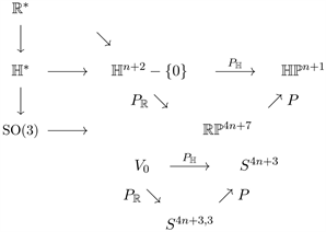
When ℍ n + 2 is viewed as the real vector space ℝ 4 n + 8 , O ( 4 n + 4,4 ) denotes the full subgroup of GL ( 4 n + 8, ℝ ) preserving the bilinear form Re   〈   ,   〉 . Consider the commutative diagrams below. The image of the pair ( O ( 4 n + 4,4 ) , V 0 ) by the projection P � is the homogeneous model of conformally flat pseudo-Riemannian geometry ( PO ( 4 n + 4,4 ) , S 4 n + 3,3 ) in which S 4 n + 3,3 = P ℝ ( V 0 ) is diffeomorphic to a quotient manifold S 4 n + 3 × ℤ 2 S 3 . The identification ℍ n + 2 = ℝ 4 n + 8 gives a natural embedding Sp ( n + 1,1 ) ⋅ Sp ( 1 ) → O ( 4 n + 4,4 ) which results a special geometry ( PSp ( n + 1,1 ) × SO ( 3 ) , S 4 n + 3,3 ) from ( PO ( 4 n + 4,4 ) , S 4 n + 3,3 ) .

As usual, the image of ( Sp ( n + 1,1 ) ⋅ Sp ( 1 ) , V 0 ) by P ℍ is spherical quarter- nionic 3 CR-geometry ( PSp ( n + 1,1 ) , S 4 n + 3 ) .

(4.3)

We describe a pseudo-Riemannian metric g 0 on S 4 n + 3,3 = S 4 n + 3 × ℤ 2 S 3 . Let S 4 n + 3 × S 3 be the product of unit spheres. For ( z , w ) ∈ S 4 n + 3 × S 3 , | z | 2 − | w | 2 = 1 − 1 = 0 so S 4 n + 3 × S 3 ⊂ V 0 . Then P ℝ ( V 0 ) = S 4 n + 3,3 induces a 2-fold covering P ℝ : S 4 n + 3 × S 3 → S 4 n + 3,3 for which P * : T ( S 4 n + 3 × S 3 ) → T S 4 n + 3,3 is an isomorphism.

Let x ∈ S 4 n + 3 × S 3 where we put P ℝ ( x ) = [ x ] . Choose y ∈ S 4 n + 3 × S 3 such that 〈 x , y 〉 = 1 . Denote by { x , y } ⊥ the orthogonal complement in ℍ n + 2 with respect to 〈   ,   〉 . As T x V 0 = { Z ∈ ℍ n + 2 | Re   〈 x , Z 〉 = 0 } , it follows T x V 0 = y Im ℍ ⊕ x ℍ ⊕ { x , y } ⊥ ⊂ ℍ n + 2 such that

T x ( S 4 n + 3 × S 3 ) = y Im ℍ ⊕ x Im ℍ ⊕ { x , y } ⊥ .

In particular, T x V 0 = x ℝ ⊕ T x ( S 4 n + 3 × S 3 ) . Note that this decomposition does not depend on the choice of points x ′ ∈ [ x ] and y ′ with 〈 x ′ , y ′ 〉 = 1 . (see [3] , Theorem 6.1]). We define a pseudo-Riemannian metric on S 4 n + 3,3 to be

g [ x ] 0 ( P ℝ * X , P ℝ * Y ) = Re 〈 X , Y 〉     ( ∀   X , Y ∈ T x ( S 4 n + 3 × S 3 ) ) . (4.4)

Noting Re 〈 y a , y a 〉 = Re 〈 x a , x a 〉 = 0 , Re 〈 x a , y a 〉 = 1 ( ∀   a ∈ Sp ( 1 ) ) and Re 〈   ,   〉 | { x , y } ⊥ is positive definite, g [ x ] 0 is a pseudo-Riemannian metric of type ( 4 n + 3,3 ) at each [ x ] ∈ S 4 n + 3,3 .

4.2. Conformal Group O ( 4 n + 4 , 4 )

It is known more or less but we need to check that O ( 4 n + 4 , 4 ) acts on S 4 n + 3 × S 3 as conformal transformations with respect to Re 〈   ,   〉 and so does PO ( 4 n + 4,4 ) on ( S 4 n + 3,3 , g 0 ) .

For any h ∈ O ( 4 n + 4,4 ) , 〈 h x , h x 〉 = 〈 x , x 〉 = 0 so h x ∈ V 0 . However h x does not necessarily belong to S 4 n + 3 × S 3 . Normalized h x , there is x ′ ∈ S 4 n + 3 × S 3 such that ( h x ) λ = x ′ for some λ ∈ ℝ + . Note [ h x ] = P ℝ ( h x ) = P ℝ ( x ′ ) . If R λ : ℍ n + 2 → ℍ n + 2 is the right multiplication defined by R λ ( z ) = z λ , then there is the commutative diagram:
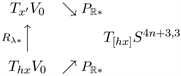
in which R * ( h * X ) = ( h * X ) λ ∈ T x ′ V 0 . As T x ′ V 0 = x ′   ℝ ⊕ T x ′ ( S 4 n + 3 × S 3 ) , we have ( h * X ) λ = x ′ μ + X ′ for some μ ∈ ℝ , X ′ ∈ T x ′ ( S 4 n + 3 × S 3 ) . Since P * ( T x ℝ * ) = P * ( x ℝ ) = 0 and P ℝ : ( O ( 4 n + 4,4 ) , V 0 ) → ( PO ( 4 n + 4,4 ) , S 4 n + 3,3 ) is equivariant, it follows

h * P ℝ * ( X ) = P ℝ * ( h * X ) = P ℝ * ( ( h * X ) λ ) = P ℝ * ( x ′ μ + X ′ ) = P ℝ * ( X ′ ) .

Similarly h * P ℝ * ( Y ) = P ℝ * ( Y ′ ) for ( h * Y ) λ = x ′ ν + Y ′ for some ν ∈ ℝ , Y ′ ∈ T x ′ ( S 4 n + 3 × S 3 ) . As Re 〈 x ′ , X ′ 〉 = Re 〈 x ′ , Y ′ 〉 = 0 , a calculation shows

g [ h x ] 0 ( h * P ℝ * ( X ) , h * P ℝ * ( Y ) ) = g [ h x ] 0 ( P ℝ * ( X ′ ) , P ℝ * ( Y ′ ) ) = Re 〈 X ′ , Y ′ 〉 = Re 〈 x ′ μ + X ′ , x ′ ν + Y ′ 〉 = Re 〈 ( h * X ) λ , ( h * Y ) λ 〉 = λ 2 Re 〈 h * X , h * Y 〉 = λ 2 Re 〈 X , Y 〉 = λ 2 g [ x ] 0 ( P ℝ * ( X ) , P ℝ * ( Y ) ) .

Hence h ∈ O ( 4 n + 4,4 ) acts as conformal transformation with respect to g 0 .

4.3. Conformal Subgroup S p ( n + 1 , 1 ) ⋅ S p ( 1 )

Let ( I , J , K ) be the standard hypercomplex structure on ℍ n + 2 defined by

I z = − z i , J z = − z j , K z = − z k .

Put Q = span ( I , J , K ) as the associated quaternionic structure. Then Re 〈   ,   〉 leaves invariant Q. The full subgroup of O ( 4 n + 4,4 ) preserving Q is isomorphic to Sp ( n + 1,1 ) ⋅ Sp ( 1 ) , i.e. the intersection of O ( 4 n + 4,4 ) with GL ( n + 2, ℍ ) ⋅ GL ( 1, ℍ ) .

Let ρ : S 3 → O ( 4 n + 4,4 ) be a faithful representation. Then the subgroup ρ ( S 3 ) preserves Q so it is contained in

( Sp ( 1 ) × ⋯ × Sp ( 1 ) ︷ n + 2 ) ⋅ Sp ( 1 ) ≤ SO ( 4 ) × ⋯ × SO ( 4 ) ︷ n + 2

which is a subgroup of SO ( 4 n + 4 ) × SO ( 4 ) .

4.4. Three Dimensional Lightlike Group

Choose S 1 ≤ S 3 and consider a representation restricted to S 1 . As we may assume that the semisimple group ρ ( S 3 ) belongs to ( Sp ( 1 ) × ⋯ × Sp ( 1 ) ) ⋅ Sp ( 1 ) , this reduces to a faithful representation: ρ : S 1 → T n + 2 ⋅ S 1 such that

ρ ( t ) = ( ( e i a 1 t , ⋯ , e i a n + 2 t ) ⋅ e i b t ) . (4.5)

Here we may assume that a i ≥ 0 are relatively prime ( i = 1 , ⋯ , n + 2 ) without loss of generality, and either b = 0 or 1. The element ρ ( t ) acts on S 4 n + 3 × S 3 ⊂ V 0 as

ρ ( t ) ( z 1 , ⋯ , z n + 1 , w ) = ( e i a 1 t z 1 , ⋯ , e i a n + 1 t z n + 1 , e i a n + 2 t w ) ⋅ e − i b t = ( e i a 1 t z 1 e − i b t , ⋯ , e i a n + 1 t z n + 1 e − i b t , e i a n + 2 t w e − i b t ) (4.6)

where | z 1 | 2 + ⋯ + | z n + 1 | 2 − | w | 2 = 0 for ( z , w ) = ( z 1 , ⋯ , z n + 1 , w ) ∈ V 0 . If X is the vector field induced by ρ ( S 1 ) at ( z , w ) , then it follows

X = ( i a 1 z 1 , ⋯ , i a n + 1 z n + 1 , i a n + 2 w ) − ( z 1 i b , ⋯ , z n + 1 i b , w i b ) . (4.7)

Proposition 7. If ρ : S 1 → T n + 2 ⋅ S 1 is a faithful lightlike 1-parameter group, then it has either one of the forms:

ρ ( t ) = ( e i t , ⋯ , e i t ) ≤ ( Sp ( 1 ) × ⋯ × Sp ( 1 ) ︷ n + 2 ) ≤ Sp ( n + 1,1 ) ⋅ { 1 } , ρ ( t ) = ( 1, ⋯ ,1 ) ⋅ e i t ≤ { 1 } ⋅ Sp ( 1 ) ≤ Sp ( n + 1,1 ) ⋅ Sp ( 1 ) . (4.8)

Proof. Case (i) b = 0 . X = ( i a 1 z 1 , ⋯ , i a n + 1 z n + 1 , i a n + 2 w ) from (4.7) so that 〈 X , X 〉 = a 1 2 | z 1 | 2 + ⋯ + a n + 1 2 | z n + 1 | 2 − a n + 2 2 | w | 2 = ( a 1 2 − a n + 2 2 ) | z 1 | 2 + ⋯ + ( a n + 1 2 − a n + 2 2 ) | z n + 1 | 2 . Since Re 〈 X , X 〉 = 0 and we assume a i ≥ 0 , it follows

a 1 = a n + 2 , ⋯ , a n + 1 = a n + 2 .

As a i ’s are relatively prime, this implies

a 1 = ⋯ = a n + 1 = a n + 2 = 1.

As a consequence ρ ( t ) = ( e i t , ⋯ , e i t ) ≤ Sp ( n + 1 , 1 ) ⋅ { 1 } . In this case note that T x ( S 4 n + 3 × S 3 ) = Im ℍ y ⊕ Im ℍ x ⊕ { x , y } ⊥ such that 〈 x , y 〉 ∈ ℝ * .

Case (ii) b = 1 . It follows from (4.7) that

X = ( i a 1 z 1 , ⋯ , i a n + 1 z n + 1 , i a n + 2 w ) − ( z 1 i , ⋯ , z n + 1 i , w i ) .

Put Y = ( i a 1 z 1 , ⋯ , i a n + 1 z n + 1 , i a n + 2 w ) , W = ( z 1 i , ⋯ , z n + 1 i , w i ) = x i such that X = Y − W and 〈 W , W 〉 = i ¯ 〈 x , x 〉 i = 0 . Calculate

〈 Y , Y 〉 = a 1 2 | z 1 | 2 + ⋯ + a n + 1 | z n + 1 | 2 − a n + 2 2 | w | 2 , 〈 Y , W 〉 = a 1 z ¯ 1 i ¯ z 1 i + ⋯ + a n + 1 z ¯ n + 1 i ¯ z n + 1 i − a n + 2 w ¯ i ¯ w i , Re 〈 Y , W 〉 = a 1 | z 1 | 2 + ⋯ + a n + 1 | z n + 1 | 2 − a n + 2 | w | = Re 〈 W , Y 〉 . (4.9)

This shows

Re 〈 X , X 〉 = Re 〈 Y − W , Y − W 〉 = Re 〈 Y , Y 〉 − 2 Re 〈 Y , W 〉 + Re 〈 W , W 〉 = R 〈 Y , Y 〉 − 2 Re 〈 Y , W 〉 = ( a 1 2 − 2 a 1 ) | z 1 | 2 + ⋯ + ( a n + 1 2 − 2 a n + 1 ) | z n + 1 | 2 − ( a n + 2 2 − 2 a n + 2 ) | w | 2 = ( ( a 1 2 − 2 a 1 ) − ( a n + 2 2 − 2 a n + 2 ) ) | z 1 | 2 + ⋯ + ( ( a n + 1 2 − 2 a n + 1 ) − ( a n + 2 2 − 2 a n + 2 ) ) | z n + 1 | 2 = ( ( a 1 − 1 ) 2 − ( a n + 2 − 1 ) 2 ) | z 1 | 2 + ⋯ + ( ( a n + 1 − 1 ) 2 − ( a n + 2 − 1 ) 2 ) | z n + 1 | 2 .

Thus

( a 1 − 1 ) 2 = ( a n + 2 − 1 ) 2 , ⋯ , ( a n + 1 − 1 ) 2 = ( a n + 2 − 1 ) 2 . (4.10)

On the other hand, we may assume in general

a 1 = ⋯ = a k = 0. a k + 1 − 1 ≤ 0 , ⋯ , a l − 1 ≤ 0. a l + 1 − 1 ≥ 0 , ⋯ , a n + 1 − 1 ≥ 0.

(ii-1). Suppose a n + 2 − 1 ≥ 0 . As 0 < a j ≤ 1 for k + 1 ≤ j ≤ l , it implies a k + 1 = ⋯ = a l = 1 . Since ( a k + 1 − 1 ) 2 = ( a n + 2 − 1 ) 2 from (4.10), it follows a n + 2 = 1 . Again from (4.10), ( a j − 1 ) 2 = 0 and so a j = 1 ( l + 1 ≤ j ≤ n + 1 ) . Note that a i ≠ 0 because ( a i − 1 ) 2 = ( a n + 2 − 1 ) 2 = 0 . Thus a 1 = a 2 = ⋯ = a n + 2 = 1 . This implies ρ ( t ) = ( e i t , ⋯ , e i t ) ⋅ e i t .

(ii-2). Suppose a n + 2 − 1 < 0 . In this case a n + 2 = 0 . By (4.10), it follows that ∀   a i ≠ 0 and a 1 = ⋯ = a l = 1 , a i = 2 ( l + 1 ≤ i ≤ n + 1 ) . Thus ρ ( t ) = ( 1 , ⋯ , 1 , e i 2 t , ⋯ , e i 2 t , 1 ) ⋅ e i t . This contradicts that nonzero a i ’s ( 1 ≤ i ≤ n + 1 ) are relatively prime.

(ii-3). Suppose a n + 2 − 1 < 0 and a 1 = a 2 = ⋯ = a n + 1 = 0 . Again a n + 2 = 0 and so ρ ( t ) = ( 1, ⋯ ,1 ) ⋅ e i t .

To complete the proof of the proposition we prove the following. Put x = ( z , w ) = ( z 1 , ⋯ , z n + 1 , w ) ∈ S 4 n + 3 × S 3 ⊂ V 0 such that 〈 x , x 〉 = 0 .

Lemma 8. Case (ii-1) does not occur.

Proof. It follows from (4.7) that

X = ( i z 1 , ⋯ , i z n + 1 , i w ) − ( z 1 i , ⋯ , z n + 1 i , w i ) = i x − x i . (4.11)

Put x = p + j q ( p , q ∈ C n+2 ) . Then X = 2 k q . As 〈 X , X 〉 = 0 implies 〈 q , q 〉 = 0 . On the other hand, the equation

0 = 〈 x , x 〉 = ( 〈 p , p 〉 + 〈 q , q 〉 ) − 2 j 〈 p ¯ , q 〉

shows 〈 p , p 〉 + 〈 q , q 〉 = 0 , 〈 p ¯ , q 〉 = 0. Note that if S 2n+1 × S 1 is the canonical subset in S 4n+3 × S 3 , then 〈 p , p 〉 = 0 if and only if p ∈ S 2n+1 × S 1 . Since X is a nontrivial vector field on S 4n+3 × S 3 , there is a point x in the open subset S = S 4n+3 × S 3 \ S 2n+1 × S 1 such that 〈 p , p 〉 ≠ 0 and thus 〈 X , X 〉 ≠ 0 on S, which contradicts that X is a lightlike vector field.

4.5. Proof of Theorem B

Applying Proposition 7 to a lightlike group S 3 we obtain:

Corollary 9. Let ρ : S 3 → O ( 4 n + 4,4 ) be a faithful representation which preserves the metric Re 〈 ,   〉 on V 0 . If ρ ( S 3 ) is a lightlike group on S 4 n + 3 × S 3 , then either one of the following holds.

ρ ( S 3 ) = diag ( Sp ( 1 ) × ⋯ × Sp ( 1 ) ) ≤ Sp ( n + 1,1 ) ⋅ { 1 } , ρ ( S 3 ) = { 1 } ⋅ Sp ( 1 ) ≤ Sp ( n + 1,1 ) ⋅ Sp ( 1 ) . (4.13)

Let ( diag ( Sp ( 1 ) × ⋯ × S p ( 1 ) ) ⋅ Sp ( 1 ) , S 4 n + 3 × S 3 ) be as in (4.13). If f : S 4 n + 3 × S 3 → S 4 n + 3 × S 3 is a map defined by f ( ( z 1 , ⋯ , z n + 1 , w ) ) = ( w ¯ z 1 , ⋯ , w ¯ z n + 1 , w ¯ ) , then for a ∈ Sp ( 1 ) , b ∈ Sp ( 1 ) ,

f ( ( a z 1 , ⋯ , a z n + 1 , a w b ¯ ) ) = ( b w ¯ z 1 , ⋯ , b w ¯ z n + 1 , b w ¯ a ¯ ) .

So the equivariant diffeomorphism f induces a quotient equivariant diffeomorphism

f ^ : ( Sp ( 1 ) , S 4 n + 3 × S 3 / ρ ( S 3 ) ) → ( diag ( Sp ( 1 ) × ⋯ × Sp ( 1 ) ) , S 4 n + 3 ) . (4.14)

We prove Theorem B of Introduction.

Proof. Suppose that the pseudo-Riemannian manifold ( M × S 3 , g ) is conformally flat. Let π = π 1 ( M ) be the fundamental group and M ˜ the universal covering of M. By the developing argument (cf. [7] ), there is a developing pair:

( ρ , Dev ) : ( π × S 3 , M ˜ × S 3 , g ˜ ) → ( O ( 4 n + 4,4 ) , S 4 n + 3 × S 3 , g 0 )

where Dev is a conformal immersion such that Dev * g 0 = u g ˜ for some positive function u on M ˜ × S 3 and ρ : π × S 3 → O ( 4 n + 4,4 ) is a holonomy homomorphism for which Dev is equivariant with respect to ρ .

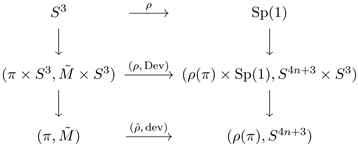
By Corollary 9, if ρ ( S 3 ) = { 1 } ⋅ Sp ( 1 ) ≤ Sp ( n + 1,1 ) ⋅ Sp ( 1 ) , then the normalizer of Sp ( 1 ) in O ( 4 n + 4,4 ) is isomorphic to Sp ( n + 1,1 ) ⋅ Sp ( 1 ) . In particular, ρ ( π × S 3 ) = ρ ( π ) × Sp ( 1 ) ≤ Sp ( n + 1,1 ) ⋅ Sp ( 1 ) where ρ ( S 3 ) = { 1 } ⋅ Sp ( 1 ) . We have the commutative diagram:

(4.15)

where ρ ( π ) ≤ PSp ( n + 1,1 ) and dev is an immersion which is ρ ^ - equivariant.

If ρ ( S 3 ) = diag ( Sp ( 1 ) × ⋯ × Sp ( 1 ) ) ≤ Sp ( n + 1,1 ) ⋅ { 1 } from (4.13), then ρ ( π × S 3 ) = ρ ( S 3 ) ⋅ ρ ( π ) ≤ diag ( Sp ( 1 ) × ⋯ × Sp ( 1 ) ) ⋅ Sp ( 1 ) . Composed f with Dev , we have an equivariant diffeomorphism f ^ ∘ dev : ( π , M ˜ ) → ( ρ ( π ) , S 4 n + 3 ) where ρ ( π ) ≤ diag ( Sp ( 1 ) × ⋯ × Sp ( 1 ) ) ≤ PSp ( n + 1,1 ) . In each case taking the developing map either dev of (4.15) or f ^ ∘ dev , a quaternionic 3 CR-manifold M is spherical, i.e. uniformized with respect to ( PSp ( n + 1,1 ) , S 4 n + 3 ) .

Conversely recall ( ω 0 , { J α 0 } α = 1 , 2 , 3 ) is the standard quaternionic 3 CR-structure on S 4 n + 3 equipped with the standard hypercomplex structure Q 0 = { J α 0 } α = 1 , 2 , 3 on D 0 . Suppose that ( ω , { J α } α = 1 , 2 , 3 ) is a spherical quaternionic 3 CR-structure on M with a quaternionic structure Q, then there exists a developing map dev : M ˜ → S 4 n + 3 such that

dev ∗ ω 0 = λ ω ˜ λ ¯

for some ℍ -valued function λ on M ˜ with a lift of quaternionic 3 CR-structure ω ˜ . In particular, dev * D = D 0 and dev * Q = Q 0 .

Let g ˜ be a pseudo-Riemannian metric on M ˜ × S 3 for ω ˜ which is a lift of g and ω to M ˜ × S 3 respectively. Put ω ′ = dev ∗ ω 0 . Let λ = u a be a function for u > 0 and a ∈ Sp ( 1 ) such that

ω ′ = u a ω ˜ a ¯ .

By the definition, recall d ω β 0 ( J γ 0 V , W ) = d ω α 0 ( V , W ) ( ∀   V , W ∈ D 0 ) . The induced quaternionic structure { J ′ α } α = 1 , 2 , 3 for ω ′ = dev ∗ ω 0 is obtained as d ( dev * ω β 0 ) ( J ′ γ X , Y ) = d ( dev * ω α 0 ) ( X , Y ) . Since d ω β 0 ( dev * J ′ γ X , dev * Y ) = d ω α 0 ( dev * X , dev * Y ) , taking V = dev * X , we obtain

dev * J ′ γ X = J γ 0 dev * X     ( ∀   X ∈ D ) . (4.16)

As dev * Q = Q 0 = span ( J α 0 , α = 1,2,3 ) , note that { J ′ α } α = 1 , 2 , 3 ∈ Q .

On the other hand, let g ′ be the pseudo-Riemannian metric on M ˜ × S 3 for ω ′ , it follows from Theorem 4

g ′ = u g ˜ . (4.17)

Take the above element a ∈ S 3 and let ρ : S 3 → S 3 be a homomorphism defined by ρ ( s ) = a s a ¯ ( ∀   s ∈ S 3 ) . Define a map dev × ρ : M ˜ × S 3 → S 4 n + 3 × S 3 which makes the diagram commutative. (Here p is the projection onto the left summand.)
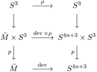
(4.18)

where both p * : ( D , { J′ α } ) → ( D , { J′ α } ) and p * : ( D 0 , { J α 0 } ) → ( D 0 , { J α 0 } ) are isomorphisms such that

p * ∘ J ′ α = J ′ α ∘ p *       and       p * ∘ J α 0 = J α 0 ∘ p *     ( α = 1 , 2 , 3 ) . (4.19)

Recall from (3.5) that g 0 = σ 0 ⊙ p * ω 0 + d p * ω α 0 ∘ J α 0 . (We write p more pre- cisely.) Consider the pull-back metric

( dev × ρ ) * g 0 ( X , Y ) = σ 0 ⊙ p * ω 0 ( ( dev × ρ ) * X , ( dev × ρ ) * Y )     + d p * ω α 0 ( J α 0 ( dev × ρ ) * X , ( dev × ρ ) * Y ) . (4.20)

Calculate the first and the second summand of (4.20) respectively.

( dev × ρ ) * ( σ 0 ⊙ p * ω 0 ) = ( dev × ρ ) * σ 0 ⊙ ( dev × ρ ) * p * ω 0 = ρ * dev * σ 0 ⊙ p * dev * ω 0 . (4.21)

d p * ω α 0 ( J α 0 ( dev × ρ ) * X , ( dev × ρ ) * Y ) = d ω α 0 ( J α 0 p * ( dev × ρ ) * X , p * ( dev × ρ ) * Y ) = d ω α 0 ( J α 0 dev * p * X , dev * p * Y )

= d ω α 0 ( dev * J ′ α p * X , dev * p * Y )

= d ω α 0 ( dev * p * J ′ α X , dev * p * Y )

= d p * dev * ω α 0 ( J ′ α X , Y ) = d ( p * dev * ω α 0 ) ∘ J ′ α ( X , Y ) . (4.22)

Thus

( dev × ρ ) * g 0 = R a ¯ *   dev * σ 0 ⊙ p * dev * ω 0 + d ( p * dev * ω α 0 ) ∘ J ′ α .

Then it follows by the construction of (3.5) that ( dev × ρ ) * g 0 is the corresponding pseudo-Riemannian metric for dev * ω 0 = ω ′ and so ( dev × ρ ) * g 0 = g ′ = u g ˜ by (4.17). Therefore ( M ˜ × S 3 , g ˜ ) is conformally flat and so is ( M × S 3 , g ) .

Conflicts of Interest

The authors declare no conflicts of interest.

References

[1] Biquard, O. (2001) Quaternionic Contact Structures, Quaternionic Structures in Mathematics and Physics, Rome, World Sci. 1999 Publishing, River Edge, NJ. 23-30.
[2] Webster, S. (1977) On the Transformation Group of a Real Hypersurfaces. Transactions of the American Mathematical Society, 231, 179-190.
[CrossRef]
[3] Alekseevsky, D.V. and Kamishima, Y. (2008) Pseudo-Conformal Quaternionic CR Structure on -Dimensional Manifolds. Annali di Matematica Pura ed Applicata, 187, 487-529.
[CrossRef]
[4] Kobayashi, S. (1970) Transformation Groups in Differential Geometry. Ergebnisse Math., 70.
[5] Lee, J. (1986) The Fefferman Metric and Pseudo Hermitian Invariants. Transactions of the American Mathematical Society, 296, 411-429.
[CrossRef]
[6] Fefferman, C. (1976) Monge-Ampère Equations, the Bergman Kernel, and Geometry of Pseudo-Convex Domains. Annals of Mathematics, 103, 395-416.
[CrossRef]
[7] Kulkarni, R. (1978) On the Principle of Uniformization. Journal of Differential Geo-metry, 13, 109-138.
[CrossRef]

Copyright © 2026 by authors and Scientific Research Publishing Inc.

Creative Commons License

This work and the related PDF file are licensed under a Creative Commons Attribution 4.0 International License.