Omer Abdalrhman^1,2*, Afif Abdalmonem^1,3, Shuangping Tao^1
1College of Mathematics and Statistics, Northwest Normal University, Lanzhou, China.
²College of Education, Shendi University, Shendi, River Nile State, Sudan.
³Faculty of Science, University of Dalanj, Dalanj, South kordofan, Sudan.
DOI: 10.4236/am.2017.84035   PDF    HTML   XML   1,710 Downloads   3,411 Views   Citations

Abstract

The aim of this paper is to study the boundedness of Calderón-Zygmund operator and their commutator on Herz Spaces with two variable exponents p(.),q(.). By applying the properties of the Lebesgue spaces with variable exponent, the boundedness of the Calderón-Zygmund operator and the commutator generated by BMO function and Calderón-Zygmund operator is obtained on Herz space.

Keywords

Calderón-Zygmund Operator, Commutator, Herz Spaces with Variable Exponent, BMO Spaces

Share and Cite:

1. Introduction

Definition 1.1. Let $T$ be a bounded linear operator from $S\left({ℝ}^n\right)$ to $S^{\prime }\left({ℝ}^n\right)$ (see [1] , [2] ). $T$ is called a standard operator if $T$ satisfies the following conditions:

1) $T$ extends to a bounded linear operator on $L^2\left({ℝ}^n\right)$ .

2) There exists a function $K\left(x,y\right)$ defined by $\left\{\left(x,y\right)\in \left({ℝ}^n\right)\times \left({ℝ}^n\right);x\ne y\right\}$ satisfies

$\left|K\left(x,y\right)\right|\le C/{\left|x-y\right|}^n,$ (1.1)

where $C>0$ .

3) $\langle Tf,g\rangle ={\displaystyle {\int }_{\left({ℝ}^n\right)}}{\displaystyle {\int }_{\left({ℝ}^n\right)}}K\left(x,y\right)f\left(y\right)g\left(x\right)\text{d}x\text{d}y,$ for $f,g\in S\left({ℝ}^n\right)$ with $\text{supp}\left(f\right)\cap \text{supp}\left(g\right)=\varnothing$

A standard operator $T$ is called a $\gamma$ -Calderón $\text{-}$ Zygmund operator if $K$ is a standard kernel satisfies:

$\left|K\left(x,y\right)-K\left(z,y\right)\right|\le C{\left|x-z\right|}^{\gamma }/{\left|x-y\right|}^{n+\gamma };$ (1.2)

$\left|K\left(y,x\right)-K\left(y,z\right)\right|\le C{\left|x-z\right|}^{\gamma }/{\left|x-y\right|}^{n+\gamma },$ (1.3)

if $\left|x-z\right|<\frac{1}{2}\left|x-y\right|$ for some $0<\gamma \le 1$ .

The bounded mean oscillation BMO space and BMO norm are defined, respectively, by

$BMO\left({ℝ}^n\right)=\left\{b\in L_{loc}^1\left({ℝ}^n\right):{\Vert b\Vert }_{BMO\left({ℝ}^n\right)}<\infty \right\},$ (1.4)

${\Vert b\Vert }_{BMO\left({ℝ}^n\right)}=\underset{B:\text{ball}}{\sup }1/\left|B\right|{\displaystyle {\int }_B}\left|b\left(x\right)-b_B\right|\text{d}x.$ (1.5)

The commutator of the Calderón-Zygmund operator is defined by

$\left[b,T\right]f\left(x\right)=b\left(x\right)Tf\left(x\right)-T\left(bf\right)\left(x\right).$ (1.6)

In 1983, J.-L. Jouné proved $\gamma$ -Calderón $\text{-}$ Zygmund operator is bounded on $L^p\left({ℝ}^n\right)$ in [3] . Coifman, Rochberg and Weiss proved that commutator [b,T] is bounded on $L^p\left({ℝ}^n\right)\left(1<p<1\right)$ (see [4] ).

Kovácik and Rákosník introduced Lebesgue spaces and Sobolev spaces with variable exponents (see [5] ). The function spaces with variable exponent has been recently obtained an increasing interest by a number of authors since many applications are found in many different fields, for example, in fluid dynamics (see [6] ), image restoration (see [7] [8] [9] ) and differential equations.

Herz spaces play an important role in harmonic analysis. After they were introduced in [10] , the boundedness of some operators and some characteriza- tions of Herz spaces with variable exponents were studied extensively (see [11] - [16] ). In 2015, Wang and Tao introduced the Herz spaces with two variable exponents $p(.),q(.)$ , and studied the parameterized Littlewood-Paley operators and their commutators on Herz spaces with variable exponents in [17] .

In this paper, we will discuss the boundedness of the Calderón-Zygmund operator $T$ and their commutator $\left[b,T\right]$ are bounded on Herz spaces with two variable exponents $p(.),q(.)$ .

2. Definitions of Function Spaces with Variable Exponent

In this section we recall some definitions. Let $\Omega$ be a measurable set in ${ℝ}^n$ with $\left|\Omega \right|>0$ . We firstly recall the definition of the Lebesgue spaces with variable exponent.

Definition 2.1. [5] Let $p(\cdot ):\Omega \to \left[1,\infty \right)$ be a measurable function. The Lebesgue space with variable exponent $L^{p(\cdot )}\left(\Omega \right)$ is defined by

$L^{p(\cdot )}\left(\Omega \right)=\left\{f\text{ismeasurable}:{\displaystyle {\int }_{\Omega }}{\left(\frac{\left|f\left(x\right)\right|}{\eta }\right)}^{p\left(x\right)}\text{d}x<\infty \text{forsomeconstant}\eta >0\right\}.$ (2.1)

For all compact $K\subset \Omega$ , the space $L_{loc}^{p(\cdot )}\left(\Omega \right)$ is defined by

$L_{loc}^{p(\cdot )}\left(\Omega \right)=\left\{f\text{ismeasurable}:f\in L^{p(\cdot )}\left(K\right)\right\}.$ (2.2)

The Lebesgue spaces $L^{p(\cdot )}\left(\Omega \right)$ is a Banach spaces with the norm defined by

${\Vert f\Vert }_{L^{p(\cdot )}\left(\Omega \right)}=\inf \left\{\eta >0:{\displaystyle {\int }_{\Omega }}{\left(\frac{\left|f\left(x\right)\right|}{\eta }\right)}^{p\left(x\right)}\text{d}x\le 1\right\}.$ (2.3)

We denote $p_{-}=ess\text{inf}\left\{p\left(x\right):x\in \Omega \right\},p_{+}=ess\sup \left\{p\left(x\right):x\in \Omega \right\}$ . Then $\mathcal{P}\left(\Omega \right)$ consists of all $p(\cdot )$ satisfying $p_{-}>1$ and $p_{+}<\infty$ . Let $M$ be the Hardy-Littlewood maximal operator. We denote $\mathcal{B}\left(\Omega \right)$ to be the set of all function $p(\cdot )\in \mathcal{P}\left(\Omega \right)$ satisfying the $M$ is bounded on $L^{p(\cdot )}\left(\Omega \right)$ .

Definition 2.2. [18] Let $p(\cdot ),q(\cdot )\in \mathcal{P}\left(\Omega \right)$ . The mixed Lebesgue sequence space with variable exponent ${\mathcal{l}}^{q(\cdot )}\left(L^{p(\cdot )}\right)$ is the collection of all sequences ${\left\{f_j\right\}}_{j=0}^{\infty }$ of the measurable functions on ${ℝ}^n$ such that

$\begin{array}{l}{\Vert {\left\{f_j\right\}}_{j=0}^{\infty }\Vert }_{{\mathcal{l}}^{q(\cdot )}\left(L^{p(\cdot )}\right)}=\inf \left\{\eta >0:Q_{{\mathcal{l}}^{q(\cdot )}\left(L^{p(\cdot )}\right)}\left(\begin{array}{c}{\left\{\frac{f_j}{\zeta }\right\}}_{j=0}^{\infty }\end{array}\right)\le 1\right\}<\infty ,\\ Q_{{\mathcal{l}}^{q(\cdot )}\left(L^{p(\cdot )}\right)}\left({\left\{f_j\right\}}_{j=0}^{\infty }\right)={\displaystyle \underset{j=0}{\overset{\infty }{\sum }}}\inf \left\{{\zeta }_j>0;{\displaystyle {\int }_{R^n}}{\left(\frac{\left|f_j\left(x\right)\right|}{{\zeta }_j^{\frac{1}{q\left(x\right)}}}\right)}^{p\left(x\right)}\text{d}x\le 1\right\}.\end{array}$ (2.4)

Let $B_k=\left\{x\in {ℝ}^n:\left|x\right|\le 2^k\right\},C_k=B_k\backslash B_{k-1},{\chi }_k={\chi }_{C_k}$ , $k\in \mathbb{Z}.$ , for $q_{+}<\infty$ , we have that

$Q_{{\mathcal{l}}^{q(\cdot )\left(L^{p(\cdot )}\right)}}\left({\left\{f_j\right\}}_{j=0}^{\infty }\right)={\displaystyle \underset{j=0}{\overset{\infty }{\sum }}}{\Vert {\left|f_j\right|}^{q(\cdot )}\Vert }_{L^{\frac{p(\cdot )}{q(\cdot )}}}.$ (2.5)

Let $B_k=\left\{x\in {ℝ}^n:\left|x\right|\le 2^k\right\},C_k=B_k\backslash B_{k-1},{\chi }_k={\chi }_{C_k}$ , $k\in \mathbb{Z}.$

Definition 2.3. [17] Let $\alpha \in {ℝ}^n,\mathrm{<mi>\; </mi>}q(\cdot ),\mathrm{<mi>\; </mi>}p(\cdot )\in \mathcal{P}\left({ℝ}^n\right)$ . The homogeneous Herz space with variable exponent ${\stackrel{\dot{}}{K}}_{p(\cdot )}^{\alpha ,q(\cdot )}\left({ℝ}^n\right)$ is defined by

${\stackrel{\dot{}}{K}}_{p(\cdot )}^{\alpha ,q(\cdot )}\left({ℝ}^n\right)=\left\{f\in L_{loc}^{p(\cdot )}\left({ℝ}^n\backslash \left\{0\right\}\right):{\Vert f\Vert }_{{\stackrel{\dot{}}{K}}_{p(\cdot )}^{\alpha ,q(\cdot )}\left({ℝ}^n\right)}<\infty \right\}.$

Equipped the norm

$\begin{array}{l}{\Vert f\Vert }_{{\stackrel{\dot{}}{K}}_{p_{(\cdot )}}^{\alpha ,q(\cdot )}\left({ℝ}^n\right)}={\Vert {\left\{2^{k\alpha }\left|f{\chi }_k\right|\right\}}_{k=0}^{\infty }\Vert }_{l^{q(\cdot )}\left(L^{p(\cdot )}\right)}\\ =\inf \left\{\eta >0:{\displaystyle \underset{k=-\infty }{\overset{\infty }{\sum }}}{\Vert {\left(\frac{2^{k\alpha }\left|f{\chi }_k\right|}{\eta }\right)}^{q(\cdot )}\Vert }_{L^{\frac{p(\cdot )}{q(\cdot )}}}\le 1\right\}.\end{array}$

Remark 2.1. [17] Let $q_1(\cdot ),q_2(\cdot )\in \mathcal{P}\left({ℝ}^n\right)$ satisfying ${\left(q_1\right)}_{+}\le {\left(q_2\right)}_{+}$ and satisfy the following results:

1) ${\stackrel{\dot{}}{K}}_{p(\cdot )}^{\alpha ,q_1(\cdot )}\left({ℝ}^n\right)\subset {\stackrel{\dot{}}{K}}_{p(\cdot )}^{\alpha ,q_2(\cdot )}\left({ℝ}^n\right).$

2) If $\frac{q_2(\cdot )}{q_1(\cdot )}\in \mathcal{P}\left({ℝ}^n\right)$ and $\frac{q_2(\cdot )}{q_1(\cdot )}\ge 1$ . For any $f\in {\stackrel{\dot{}}{K}}_{p(\cdot )}^{\alpha ,q(\cdot )}\left({ℝ}^n\right)$ , by using Lemma 3.7 and Remark 2.2, we have

$\begin{array}{c}{\displaystyle \underset{k=-\infty }{\overset{\infty }{\sum }}}{\Vert {\left(\frac{2^{k\alpha }\left|f{\chi }_k\right|}{\eta }\right)}^{q_2(\cdot )}\Vert }_{L^{\frac{p(\cdot )}{q_2(\cdot )}}}\le {\displaystyle \underset{k=-\infty }{\overset{\infty }{\sum }}}{\Vert {\left(\frac{2^{k\alpha }\left|f{\chi }_k\right|}{\eta }\right)}^{q_1(\cdot )}\Vert }_{L^{\frac{p(\cdot )}{q_1(\cdot )}}}^{p_v}\\ \le {\left\{{\displaystyle \underset{k=-\infty }{\overset{\infty }{\sum }}}{\Vert {\left(\frac{2^{k\alpha }\left|f{\chi }_k\right|}{\eta }\right)}^{q_1(\cdot )}\Vert }_{L^{\frac{p(\cdot )}{q_1(\cdot )}}}^{p_h}\right\}}^{p_{*}}\le 1.\end{array}$

where

$p_v=\{\begin{array}{l}{\left(\frac{q_2(\cdot )}{q_1(\cdot )}\right)}_{-},\frac{2^{k\alpha }\left|f{\chi }_k\right|}{\eta }\le 1,\hfill \\ {\left(\frac{q_2(\cdot )}{q_1(\cdot )}\right)}_{+},\frac{2^{k\alpha }\left|f{\chi }_k\right|}{\eta }>1.\hfill \end{array}$

$p_{*}=\{\begin{array}{l}\underset{v\in \mathbb{N}}{{\displaystyle \min }}{p}_v,{\displaystyle \underset{v=0}{\overset{\infty }{\sum }}}{a}_v\le 1,\hfill \\ \underset{v\in \mathbb{N}}{{\displaystyle \max }}{p}_v,{\displaystyle \underset{v=0}{\overset{\infty }{\sum }}}{a}_v>1.\hfill \end{array}$

This implies that ${\stackrel{\dot{}}{K}}_{p(\cdot )}^{\alpha ,q_1(\cdot )}\left({ℝ}^n\right)\subset {\stackrel{\dot{}}{K}}_{p(\cdot )}^{\alpha ,q_2(\cdot )}\left({ℝ}^n\right)$ .

Remark 2.2. Let $v\in \mathbb{N},\mathrm{<mi>\; </mi>}{a}_v\ge 0,\mathrm{<mi>\; </mi>1}\le p_v<\infty$ . Then we have

${\displaystyle \underset{v=0}{\overset{\infty }{\sum }}}{a}_v\le {\left({\displaystyle \underset{v=0}{\overset{\infty }{\sum }}}{a}_h\right)}^{p_{*}},$

where

$p_{*}=\{\begin{array}{l}\underset{v\in \mathbb{N}}{{\displaystyle \min }}{p}_v,{\displaystyle \underset{v=0}{\overset{\infty }{\sum }}}{a}_v\le 1,\hfill \\ \underset{v\in \mathbb{N}}{{\displaystyle \max }}{p}_v,{\displaystyle \underset{v=0}{\overset{\infty }{\sum }}}{a}_v>1.\hfill \end{array}$

3. Properties and Lemmas of Variable Exponent

In this section, we recall some properties and some lemmas of variable exponent belonging to the class $\mathcal{B}\left({ℝ}^n\right)$ .

Proposition 3.1. [19] If $p(\cdot )\in \mathcal{P}\left({ℝ}^n\right)$ satisfies

$\left|p\left(x\right)-p\left(y\right)\right|\le \frac{-C}{\text{Log}\left(\left|x-y\right|\right)},\left|x-y\right|\le 1/2;$ (3.1)

$\left|p\left(x\right)-p\left(y\right)\right|\le \frac{C}{\text{Log}\left(e+\left|x\right|\right)},\left|y\right|\ge \left|x\right|.$ (3.2)

Hence we have $p(\cdot )\in \mathcal{B}\left({ℝ}^n\right)$ .

Lemma 3.1. [5] Given $p(\cdot ):{ℝ}^n\to \left[1,\infty \right)$ have that for all functions $f$ and $g$ ,

${\displaystyle {\int }_{{ℝ}^n}}\left|f\left(x\right)g\left(x\right)\right|\text{d}x\le C{\Vert f\Vert }_{L^{p(\cdot )}\left({ℝ}^n\right)}{\Vert g\Vert }_{L^{p^{\prime }(\cdot )}\left({ℝ}^n\right)}.$ (3.3)

where $C_p=1+\frac{1}{p_{-}}-\frac{1}{p_{+}}$ .

Lemma 3.2. [5] Suppose that $p(\cdot ),\mathrm{<mi>\; </mi>}{p}_1(\cdot ),\mathrm{<mi>\; </mi>}{p}_2(\cdot )\in \mathcal{P}\left({ℝ}^n\right)$ , for any $f\in L^{p_1(\cdot )}\left({ℝ}^n\right),\mathrm{<mi>\; </mi>}g\in L^{p_2(\cdot )}\left({ℝ}^n\right)$ , when $\frac{1}{p(\cdot )}=\frac{1}{p_2(\cdot )}+\frac{1}{p_1(\cdot )}$ , we get

${\Vert f\left(x\right)g\left(x\right)\Vert }_{L^{p(\cdot )}\left({ℝ}^n\right)}\le C{\Vert g\left(x\right)\Vert }_{L^{p_2}\left({ℝ}^n\right)}{\Vert f\left(x\right)\Vert }_{L^{p_1(\cdot )}\left({ℝ}^n\right)},$ (3.4)

where $C_{p_1,p_2}={\left[1+\frac{1}{p_{1-}}-\frac{1}{p_{1+}}\right]}^{\frac{1}{p_{-}}}$ .

Proposition 3.2. [20] Let $p(\cdot )\in \mathcal{B}\left({ℝ}^n\right)$ and $T$ be a Calderón $\text{-}$ Zygmund operator. Then we have

${\Vert Tf\Vert }_{L^{p(\cdot )}\left({ℝ}^n\right)}\le C{\Vert f\Vert }_{L^{p(\cdot )}\left({ℝ}^n\right)}.$ (3.5)

Lemma 3.3. [20] Let $p(\cdot )\in \mathcal{B}\left({ℝ}^n\right),b\in \text{BMO}$ function and $T$ be a Calderón $\text{-}$ Zygmund operator.Then

${\Vert \left[b,T\right]f\Vert }_{L^{p(\cdot )}\left({ℝ}^n\right)}\le C{\Vert b\Vert }_{\text{BMO}\left({ℝ}^n\right)}{\Vert f\Vert }_{L^{p(\cdot )}\left({ℝ}^n\right)}$ (3.6)

Lemma 3.4. [11] Let $b\in \text{BMO}\left({ℝ}^n\right)$ . If $i,j\in \mathbb{Z}$ with $i<j$ , then we have

1. $C^{-1}{\Vert b\Vert }_{\text{BMO}\left({ℝ}^n\right)}\le \underset{B}{\sup }\frac{1}{{\Vert {\chi }_B\Vert }_{L^{p(\cdot )}\left({ℝ}^n\right)}}{\Vert \left(b-b_B\right){\chi }_B\Vert }_{L^{p(\cdot )}\left({ℝ}^n\right)}\le C{\Vert b\Vert }_{\text{BMO}\left({ℝ}^n\right)}.$

2. ${\Vert \left(b-b_{B_i}\right){\chi }_{B_j}\Vert }_{L^{q(\cdot )}\left({ℝ}^n\right)}\le C\left(j-i\right){\Vert b\Vert }_{\text{BMO}\left({ℝ}^n\right)}{\Vert {\chi }_{B_j}\Vert }_{L^{q(\cdot )}\left({ℝ}^n\right)}.$

Lemma 3.5. [21] Let $p_u(\cdot )\in \mathcal{B}\left({ℝ}^n\right)\left(u=1,2\right)$ , then there exist constants $0<{\iota }_{u1},{\iota }_{u2}<1$ , and $C>0$ such that for all balls $B\subset {ℝ}^n$ and all measurable subset $R\subset B$ ,

$\frac{{\Vert {\chi }_R\Vert }_{L^{p_u(\cdot )}\left({ℝ}^n\right)}}{{\Vert {\chi }_B\Vert }_{L^{p_u(\cdot )}\left({ℝ}^n\right)}}\le C{\left(\frac{\left|R\right|}{\left|B\right|}\right)}^{{\iota }_{u1}},\frac{{\Vert {\chi }_R\Vert }_{L^{{p^{\prime }}_u(\cdot )}\left({ℝ}^n\right)}}{{\Vert {\chi }_B\Vert }_{L^{{p^{\prime }}_u(\cdot )}\left({ℝ}^n\right)}}\le C{\left(\frac{\left|R\right|}{\left|B\right|}\right)}^{{\iota }_{u2}}.$ (3.7)

Lemma 3.6. [11] If $p(\cdot )\in \mathcal{B}\left({ℝ}^n\right)$ , there exist a constant $C>0$ such that for any balls B in ${ℝ}^n$ , we have

$\frac{1}{\left|B\right|}{\Vert {\chi }_B\Vert }_{L^{p(\cdot )}\left({ℝ}^n\right)}{\Vert {\chi }_B\Vert }_{L^{p^{\prime }(\cdot )}\left({ℝ}^n\right)}\le C.$ (3.8)

Lemma 3.7. [17] Suppose that $p(\cdot ),\mathrm{<mi>\; </mi>}q(\cdot )\in \mathcal{P}\left({\mathcal{B}}^n\right)$ . If $f\in L^{p(\cdot )q(\cdot )}$ , then

$\min \left({\Vert f\Vert }_{L^{p(\cdot )q(\cdot )}}^{q_{+}},{\Vert f\Vert }_{L^{p(\cdot )q(\cdot )}}^{q_{-}}\right)\le {\Vert {\left|f\right|}^{q(\cdot )}\Vert }_{L^{p(\cdot )}}\le \max \left({\Vert f\Vert }_{L^{p(\cdot )q(\cdot )}}^{q_{+}},{\Vert f\Vert }_{L^{p(\cdot )q(\cdot )}}^{q_{-}}\right).$ (3.9)

4. The Main Theorems and Their Proofs

Theorem 4.1. Suppose that $p_1(\cdot )\in \mathcal{B}\left({ℝ}^n\right),\mathrm{<mi>\; </mi>}{q}_1(\cdot ),\mathrm{<mi>\; </mi>}{q}_2(\cdot )\in \mathcal{P}\left({ℝ}^n\right)$ with ${\left(q_2\right)}_{-}\ge {\left(q_1\right)}_{+}$ . If $-n{\iota }_{12}<\alpha <n{\iota }_{11}$ with ${\iota }_{11},{\iota }_{12}$ as defined in Lemma 3.5, then the operator $T$ is bounded from ${\stackrel{\dot{}}{K}}_{p_1(\cdot )}^{\alpha ,q_2(\cdot )}\left({ℝ}^n\right)$ to ${\stackrel{\dot{}}{K}}_{p_1(\cdot )}^{\alpha ,q_1(\cdot )}\left({ℝ}^n\right)$ .

Proof Let $h\left(x\right)\in {\stackrel{\dot{}}{K}}_{p_1(\cdot )}^{\alpha ,q_1(\cdot )}\left({ℝ}^n\right)$ . We write

$h\left(x\right)={\displaystyle \underset{j=-\infty }{\overset{\infty }{\sum }}}h\left(x\right){\chi }_j={\displaystyle \underset{j=-\infty }{\overset{\infty }{\sum }}}{h}_j\left(x\right).$

By Definition 2.3, we have

#Math_135# (4.1)

Since

$\begin{array}{c}{\Vert {\left(\frac{2^{k\alpha }\left|T\left(h\right){\chi }_k\right|}{\eta }\right)}^{q_2(\cdot )}\Vert }_{L^{\frac{p_1(\cdot )}{q_2(\cdot )}}}\le {\Vert {\left(\frac{2^{k\alpha }\left|{\displaystyle {\sum }_{j=-\infty }^{\infty }T\left(h_j\right){\chi }_k}\right|}{{\displaystyle {\sum }_{i=1}^3{\eta }_{1i}}}\right)}^{q_2(\cdot )}\Vert }_{L^{\frac{p_1(\cdot )}{q_2(\cdot )}}}\\ \le {\Vert {\left(\frac{2^{k\alpha }\left|{\displaystyle {\sum }_{j=-\infty }^{k-2}T\left(h_j\right){\chi }_k}\right|}{{\eta }_{11}}\right)}^{q_2(\cdot )}\Vert }_{L^{\frac{p_1(\cdot )}{q_2(\cdot )}}}\\ +{\Vert {\left(\frac{2^{k\alpha }\left|{\displaystyle {\sum }_{j=k-2}^{k+2}T\left(h_j\right){\chi }_k}\right|}{{\eta }_{12}}\right)}^{q_2(\cdot )}\Vert }_{L^{\frac{p_1(\cdot )}{q_2(\cdot )}}}\\ +{\Vert {\left(\frac{2^{k\alpha }\left|{\displaystyle {\sum }_{j=k+2}^{\infty }T\left(h_j\right){\chi }_k}\right|}{{\eta }_{13}}\right)}^{q_2(\cdot )}\Vert }_{L^{\frac{p_1(\cdot )}{q_2(\cdot )}}},\end{array}$ (4.2)

where

${\eta }_{11}={\Vert {\left\{2^{k\alpha }\left|{\displaystyle \underset{j=-\infty }{\overset{k-2}{\sum }}}T\left(h_j\right){\chi }_k\right|\right\}}_{k=-\infty }^{\infty }\Vert }_{{\mathcal{l}}^{q_2(\cdot )}\left(L^{p_1(\cdot )}\right)},$ (4.3)

${\eta }_{12}={\Vert {\left\{2^{k\alpha }\left|{\displaystyle \underset{j=k-2}{\overset{k+2}{\sum }}}T\left(h_j\right){\chi }_k\right|\right\}}_{k=-\infty }^{\infty }\Vert }_{{\mathcal{l}}^{q_2(\cdot )}\left(L^{p_1(\cdot )}\right)},$ (4.4)

${\eta }_{13}={\Vert {\left\{2^{k\alpha }\left|{\displaystyle \underset{j=k+2}{\overset{\infty }{\sum }}}T\left(h_j\right){\chi }_k\right|\right\}}_{k=-\infty }^{\infty }\Vert }_{{\mathcal{l}}^{q_2(\cdot )}\left(L^{p_1(\cdot )}\right)},$

and

$\eta ={\displaystyle \underset{i=1}{\overset{3}{\sum }}}{\eta }_{1i}.$

Thus,

${\displaystyle \underset{k=-\infty }{\overset{\infty }{\sum }}}{\Vert {\left(\frac{2^{k\alpha }\left|T\left(h\right){\chi }_k\right|}{\eta }\right)}^{q_2(\cdot )}\Vert }_{L^{\frac{p_1(\cdot )}{q_2(\cdot )}}}\le C.$

We easily see that

${\Vert T\left(h\right)\Vert }_{{\stackrel{\dot{}}{K}}_{p_1(\cdot )}^{\alpha ,q_2(\cdot )}\left({ℝ}^n\right)}\le C\eta =C{\displaystyle \underset{i=1}{\overset{3}{\sum }}}{\eta }_{1i}.$ (4.6)

This implies that we only need to prove ${\eta }_{11},{\eta }_{12},{\eta }_{13}\le C{\Vert h\Vert }_{{\stackrel{\dot{}}{K}}_{p_1(\cdot )}^{\alpha ,q_1(\cdot )}\left({ℝ}^n\right)}$ . Denote ${\eta }_{10}={\Vert h\Vert }_{{\stackrel{\dot{}}{K}}_{p_1(\cdot )}^{\alpha ,q_1(\cdot )}\left({ℝ}^n\right)}.$

First, we consider ${\eta }_{12}$ . By virtue of Lemma 3.7, we get

$\begin{array}{l}{\displaystyle \underset{k=-\infty }{\overset{\infty }{\sum }}}{\Vert {\left(\frac{2^{k\alpha }\left|{\displaystyle {\sum }_{j=k-2}^{k+2}T\left(h_j\right){\chi }_k}\right|}{{\eta }_{10}}\right)}^{q_2(\cdot )}\Vert }_{L^{\frac{p_1(\cdot )}{q_2(\cdot )}}}\\ \le {\displaystyle \underset{k=-\infty }{\overset{\infty }{\sum }}}{\Vert \frac{2^{k\alpha }\left|{\displaystyle {\sum }_{j=k-2}^{k+2}T\left(h_j\right){\chi }_k}\right|}{{\eta }_{10}}\Vert }_{L^{p_1(\cdot )}}^{{\left(q_2^1\right)}_k}\\ \le {\displaystyle \underset{k=-\infty }{\overset{\infty }{\sum }}}{\left({\Vert \frac{2^{k\alpha }\left|{\displaystyle {\sum }_{j=k-2}^{k+2}T\left(h_j\right){\chi }_k}\right|}{{\eta }_{10}}\Vert }_{L^{p_1(\cdot )}}\right)}^{{\left(q_2^1\right)}_k},\end{array}$ (4.7)

where,

${\left(q_2^1\right)}_k=\{\begin{array}{l}{\left(q_2\right)}_{-},{\Vert {\left(\frac{2^{k\alpha }\left|{\displaystyle {\sum }_{j=k-2}^{k+2}T\left(h_j\right){\chi }_k}\right|}{{\eta }_{10}}\right)}^{q_2(\cdot )}\Vert }_{L^{\frac{p_1(\cdot )}{q_2(\cdot )}}}\le 1,\hfill \\ {\left(q_2\right)}_{+},{\Vert {\left(\frac{2^{k\alpha }\left|{\displaystyle {\sum }_{j=k-2}^{k+2}T\left(h_j\right){\chi }_k}\right|}{{\eta }_{10}}\right)}^{q_2(\cdot )}\Vert }_{L^{\frac{p_1(\cdot )}{q_2(\cdot )}}}>1.\hfill \end{array}$

In the above, we use the Proposition 3.2 and Remark 2.2. Since $h\left(x\right)\in {\stackrel{\dot{}}{K}}_{p_1(\cdot )}^{\alpha ,q_1(\cdot )}\left({ℝ}^n\right)$ , we have ${\Vert \frac{2^{k\alpha }\left|h{\chi }_k\right|}{{\eta }_{10}}\Vert }_{L^{p_1(\cdot )}}\le 1$ and ${\displaystyle {\sum }_{k=-\infty }^{\infty }}{\Vert {\left(\frac{2^{k\alpha }\left|h{\chi }_k\right|}{{\eta }_{10}}\right)}^{q_1(\cdot )}\Vert }_{L^{\frac{p_1(\cdot )}{q_1(\cdot )}}}\le 1$ , we get

$\begin{array}{l}{\displaystyle \underset{k=-\infty }{\overset{\infty }{\sum }}}{\Vert {\left(\frac{2^{k\alpha }\left|{\displaystyle {\sum }_{j=k-2}^{k+2}T\left(h_j\right){\chi }_k}\right|}{{\eta }_{10}}\right)}^{q_2(\cdot )}\Vert }_{L^{\frac{p_1(\cdot )}{q_2(\cdot )}}}\\ \le C{\displaystyle \underset{k=-\infty }{\overset{\infty }{\sum }}}{\left({\displaystyle \underset{j=k-2}{\overset{k+2}{\sum }}}{\Vert \frac{2^{k\alpha }\left|h_j\right|}{{\eta }_{10}}\Vert }_{L^{p_1(\cdot )}}\right)}^{{(q_2^1)}_k}\\ \le C{\displaystyle \underset{k=-\infty }{\overset{\infty }{\sum }}}{\Vert \frac{2^{k\alpha }\left|h{\chi }_k\right|}{{\eta }_{10}}\Vert }_{L^{p_1(\cdot )}}^{{\left(q_2^1\right)}_k}\\ \le C{\displaystyle \underset{k=-\infty }{\overset{\infty }{\sum }}}{\Vert {\left(\frac{2^{k\alpha }\left|h{\chi }_k\right|}{{\eta }_{10}}\right)}^{q_1(\cdot )}\Vert }_{L^{\frac{p_1(\cdot )}{q_1(\cdot )}}}^{\frac{{\left(q_2^1\right)}_k}{{\left(q_1\right)}_{+}}}\\ \le C{\left\{{\displaystyle \underset{k=-\infty }{\overset{\infty }{\sum }}}{\Vert {\left(\frac{2^{k\alpha }\left|h{\chi }_k\right|}{{\eta }_{10}}\right)}^{q_1(\cdot )}\Vert }_{L^{\frac{p_1(\cdot )}{q_1(\cdot )}}}\right\}}^{q_{*}}\\ \le C.\end{array}$

Here ${\left(p_1\right)}_{+}\le {\left(p_2\right)}_{-}\le {\left(q_2^1\right)}_k$ and $q_{*}=\underset{k\in N}{\min }\frac{{\left(q_2^1\right)}_k}{{\left(q_1\right)}_{+}}$ . That is

${\eta }_{12}\le C{\eta }_{10}\le C{\Vert h\Vert }_{{\stackrel{\dot{}}{K}}_{p_1(\cdot )}^{\alpha ,q_1(\cdot )}\left({ℝ}^n\right)}.$ (4.8)

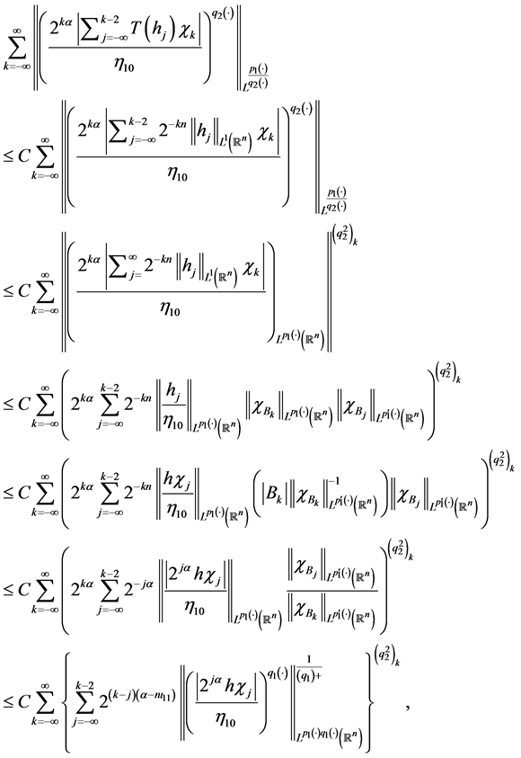
Let us now turn to estimate ${\eta }_{11}$ . Noting that $x\in A_j$ and $j\le k-2$ , by the generalized Hölder's inequality and the Minkowski’s inequality, we get

$\begin{array}{c}\left|T{h}_j\left(x\right)\right|\le {\displaystyle {\int }_{A_j}}\left|K\left(x,y\right)h_j\left(y\right)\right|\text{d}y\\ \le C{\displaystyle {\int }_{A_j}}\left|h_j\left(y\right)\right|/{\left|x-y\right|}^n\text{d}y\\ \le C{2}^{-kn}{\displaystyle {\int }_{A_j}}\left|h_j\left(y\right)\right|\text{d}y\\ \le C{2}^{-kn}{\Vert h_j\Vert }_{L^1\left({ℝ}^n\right)}.\end{array}$ (4.9)

By Lemmas 3.5-3.7 and the fact that ${\Vert \frac{2^{j\alpha }\left|h{\chi }_j\right|}{{\eta }_{10}}\Vert }_{L^{p_1(\cdot )q_1}}\le 1$ , we easily see that

(4.10)

where

${\left(q_2^2\right)}_k=\{\begin{array}{l}{\left(q_2\right)}_{-},{\Vert {\left(\frac{2^{k\alpha }\left|{\displaystyle {\sum }_{j=-\infty }^{k-2}T\left(h_j\right){\chi }_k}\right|}{{\eta }_{10}}\right)}^{q_2(\cdot )}\Vert }_{L^{\frac{p_1(\cdot )}{q_2(\cdot )}}}\le 1,\hfill \\ {\left(q_2\right)}_{+},{\Vert {\left(\frac{2^{k\alpha }\left|{{\displaystyle {\sum }_{j=-\infty }^{k-2}T\left(h_j\right)\chi }}_k\right|}{{\eta }_{10}}\right)}^{q_2(\cdot )}\Vert }_{L^{\frac{p_1(\cdot )}{q_2(\cdot )}}}>1.\hfill \end{array}$

Therefore, if ${\left(q_1\right)}_{+}<1$ and ${\left(p_1\right)}_{+}\le {\left(p_2\right)}_{-}\le {\left(q_2^2\right)}_k$ , we can get

$\begin{array}{l}{\displaystyle \underset{k=-\infty }{\overset{\infty }{\sum }}}{\Vert {\left(\frac{2^{k\alpha }\left|{\displaystyle {\sum }_{j=-\infty }^{k-2}T\left(h_j\right){\chi }_k}\right|}{{\eta }_{10}}\right)}^{q_2(\cdot )}\Vert }_{L^{\frac{p_1(\cdot )}{q_2(\cdot )}}}\\ \le C{\left\{{\displaystyle \underset{j=-\infty }{\overset{\infty }{\sum }}}{\Vert {\left(\frac{\left|2^{j\alpha }h{\chi }_j\right|}{{\eta }_{10}}\right)}^{q_1(\cdot )}\Vert }_{L^{p_1(\cdot )q_1(\cdot )}}{\displaystyle \underset{k=j+2}{\overset{\infty }{\sum }}}{2}^{\left(k-j\right)\left(\alpha -n{\iota }_{11}\right)}\right\}}^{q_{*}}\\ \le C,\end{array}$

where $q_{*}=\underset{k\in \mathbb{N}}{\min }\frac{{\left(q_2^1\right)}_k}{{\left(q_1\right)}_{+}}$ .

If ${\left(q_1\right)}_{+}\ge 1$ and ${\left(q_2^2\right)}_k\ge {\left(q_2\right)}_{-}\ge {\left(q_2\right)}_{+}\ge 1$ . By Remark 2.2 and applying the generalized Hölder’s inequality, we obtain

$\begin{array}{l}{\displaystyle \underset{k=-\infty }{\overset{\infty }{\sum }}}{\Vert {\left(\frac{2^{k\alpha }\left|{\displaystyle {\sum }_{j=-\infty }^{k-2}T\left(h_j\right){\chi }_k}\right|}{{\eta }_{10}}\right)}^{q_2(\cdot )}\Vert }_{L^{\frac{p_1(\cdot )}{q_2(\cdot )}}}\\ \le C{\displaystyle \underset{k=-\infty }{\overset{\infty }{\sum }}}{\left\{{\displaystyle \underset{j=-\infty }{\overset{k-2}{\sum }}}\left(k-j\right)2^{\left(k-j\right)\left(\alpha -n{\iota }_{11}\right){\left(q_1\right)}_{+}/2}{\Vert {\left(\frac{\left|2^{j\alpha }h{\chi }_j\right|}{{\eta }_{10}}\right)}^{q_1(\cdot )}\Vert }_{L^{p_1(\cdot )q_1(\cdot )}}\right\}}^{\frac{{\left(q_2^2\right)}_k}{\left(q_1\right)+}}\\ \times {\left({\displaystyle \underset{j=-\infty }{\overset{k-2}{\sum }}}{2}^{\left(k-j\right)\left(\alpha -n{\iota }_{11}\right){\left({\left(q_1\right)}_{+}\right)}^{\prime }/2}\right)}^{\frac{{\left(q_2^2\right)}_k}{{\left(\left(q_1\right)+\right)}^{\prime }}}\\ \le C{\left\{{\displaystyle \underset{j=-\infty }{\overset{\infty }{\sum }}}{\Vert {\left(\frac{\left|2^{j\alpha }h{\chi }_j\right|}{{\eta }_{10}}\right)}^{q_1(\cdot )}\Vert }_{L^{p_1(\cdot )q_1(\cdot )}}{\displaystyle \underset{k=j+2}{\overset{\infty }{\sum }}}{2}^{\left(k-j\right)\left(\alpha -n{\iota }_{11}\right){\left(q_1\right)}_{+}/2}\right\}}^{q_{*}}\\ \le C,\end{array}$

where $q_{*}=\underset{k\in \mathbb{N}}{\min }\frac{{\left(q_2^2\right)}_k}{{\left(q_1\right)}_{+}}$ .

Hence, we see that

${\eta }_{11}\le C{\eta }_{10}\le C{\Vert h\Vert }_{{\stackrel{\dot{}}{K}}_{p_1(\cdot )}^{\alpha ,q_1(\cdot )}\left({ℝ}^n\right)}.$ (4.11)

Finally, we estimate ${\eta }_{13}$ . Noting that for each $x\in A_j$ and $j\ge k+2$ , we have

$\left|T{h}_j\left(x\right)\right|\le {\displaystyle {\int }_{A_j}}\left|K\left(x,y\right)h_j\left(y\right)\right|\text{d}y\le C{\displaystyle {\int }_{A_j}}\left|h_j\left(y\right)\right|/{\left|x-y\right|}^n\text{d}y\le C{2}^{-jn}{\Vert h_j\Vert }_{L^1\left({ℝ}^n\right)}.$ (4.12)

By Lemma 3.7 and ${\Vert \frac{2^{j\alpha }\left|h{\chi }_j\right|}{{\eta }_{10}}\Vert }_{L^{p_1(\cdot )q_1(\cdot )}}\le 1$ , we get

(4.13)

where

${\left(q_2^3\right)}_k=\{\begin{array}{l}{\left(q_2\right)}_{-},{\Vert {\left(\frac{2^{k\alpha }\left|{\displaystyle {\sum }_{j=k+2}^{\infty }T\left(h_j\right){\chi }_k}\right|}{{\eta }_{10}}\right)}^{q_2(\cdot )}\Vert }_{L^{\frac{p_1(\cdot )}{q_2(\cdot )}}}\le 1,\hfill \\ {\left(q_2\right)}_{+},{\Vert {\left(\frac{2^{k\alpha }\left|{\displaystyle {\sum }_{j=k+2}^{\infty }T\left(h_j\right){\chi }_k}\right|}{{\eta }_{10}}\right)}^{q_2(\cdot )}\Vert }_{L^{\frac{p_1(\cdot )}{q_2(\cdot )}}}>1.\hfill \end{array}$

Then we have ${\eta }_{13}\le C{\eta }_{10}\le C{\Vert h\Vert }_{{\stackrel{\dot{}}{K}}_{p_1(\cdot )}^{\alpha ,q_1(\cdot )}\left({ℝ}^n\right)}$ , by using the same argument in ${\eta }_{11}$ . Thus, we prove Theorem 4.1. $�$

Theorem 4.2. Let $b\in \text{BMO}\left({ℝ}^n\right)$ . Suppose that $p_1(\cdot )\in \mathcal{B}\left({ℝ}^n\right),\mathrm{<mi>\; </mi>}{q}_1(\cdot ),\mathrm{<mi>\; </mi>}{q}_2(\cdot )\in \mathcal{P}\left({ℝ}^n\right)$ with ${\left(q_2\right)}_{-}\ge {\left(q_1\right)}_{+}$ . If $-n{\iota }_{12}<\alpha <n{\iota }_{11}$ with ${\iota }_{11}\mathrm{,}{\iota }_{12}$ as defined in lemma 3.5, then the commutator $\left[b\mathrm{,}T\right]$ is bounded from ${\stackrel{\dot{}}{K}}_{p_1(\cdot )}^{\alpha ,q_2(\cdot )}\left({ℝ}^n\right)$ to ${\stackrel{\dot{}}{K}}_{p_1(\cdot )}^{\alpha ,q_1(\cdot )}\left({ℝ}^n\right)$ .

Proof Let $h\left(x\right)\in {\stackrel{\dot{}}{K}}_{p_1(\cdot )}^{\alpha \mathrm{,}{q}_1(\cdot )}\left({ℝ}^n\right)\mathrm{,}b\in \text{BMO}\left({ℝ}^n\right)$ .We write

$h\left(x\right)={\displaystyle \underset{j=-\infty }{\overset{\infty }{\sum }}}h\left(x\right){\chi }_j={\displaystyle \underset{j=-\infty }{\overset{\infty }{\sum }}}{h}_j\left(x\right)$

By virtue of the definition of ${\stackrel{\dot{}}{K}}_{p(\cdot )}^{\alpha ,q(\cdot )}\left({ℝ}^n\right)$ , we have

${\Vert \left[b,T\right]\left(h\right)\Vert }_{{\stackrel{\dot{}}{K}}_{p_1(\cdot )}^{\alpha ,q_2(\cdot )}\left({ℝ}^n\right)}=\inf \left\{\eta >0:{\displaystyle \underset{k=-\infty }{\overset{\infty }{\sum }}}{\Vert {\left(\frac{2^{k\alpha }\left|\left[b,T\right]\left(h\right){\chi }_k\right|}{\eta }\right)}^{q_2(\cdot )}\Vert }_{L^{\frac{p_1(\cdot )}{q_2(\cdot )}}}\le 1\right\}.$ (4.14)

Since

$\begin{array}{l}{\Vert {\left(\frac{2^{k\alpha }\left|\left[b,T\right]\left(h\right){\chi }_k\right|}{\eta }\right)}^{q_2(\cdot )}\Vert }_{L^{\frac{p_1(\cdot )}{q_2(\cdot )}}}\le {\Vert {\left(\frac{2^{k\alpha }\left|{\displaystyle {\sum }_{j=-\infty }^{k-2}\left[b,T\right]\left(h_j\right){\chi }_k}\right|}{{\displaystyle {\sum }_{i=1}^3{\eta }_{2i}}}\right)}^{q_2(\cdot )}\Vert }_{L^{\frac{p_1(\cdot )}{q_2(\cdot )}}}\\ \le {\Vert {\left(\frac{2^{k\alpha }\left|{\displaystyle {\sum }_{j=-\infty }^{\infty }\left[b,T\right]\left(h_j\right){\chi }_k}\right|}{{\eta }_{21}}\right)}^{q_2(\cdot )}\Vert }_{L^{\frac{p_1(\cdot )}{q_2(\cdot )}}}+{\Vert {\left(\frac{2^{k\alpha }\left|{\displaystyle {\sum }_{j=k-2}^{k+2}\left[b,T\right]\left(h_j\right){\chi }_k}\right|}{{\eta }_{22}}\right)}^{q_2(\cdot )}\Vert }_{L^{\frac{p_1(\cdot )}{q_2(\cdot )}}}\\ +{\Vert {\left(\frac{2^{k\alpha }\left|{\displaystyle {\sum }_{j=k+2}^{\infty }\left[b,T\right]\left(h_j\right){\chi }_k}\right|}{{\eta }_{23}}\right)}^{q_2(\cdot )}\Vert }_{L^{\frac{p_1(\cdot )}{q_2(\cdot )}}}.\end{array}$ (4.15)

Let

${\eta }_{21}={\Vert {\left\{2^{k\alpha }\left|{\displaystyle \underset{j=-\infty }{\overset{k-2}{\sum }}}\left[b,T\right]\left(h_j\right){\chi }_k\right|\right\}}_{k=-\infty }^{\infty }\Vert }_{{\mathcal{l}}^{q_2(\cdot )}\left(L^{p_1(\cdot )}\right)},$ (4.16)

${\eta }_{22}={\Vert {\left\{2^{k\alpha }\left|{\displaystyle \underset{j=k-2}{\overset{k+2}{\sum }}}\left[b,T\right]\left(h_j\right){\chi }_k\right|\right\}}_{k=-\infty }^{\infty }\Vert }_{{\mathcal{l}}^{q_2(\cdot )}\left(L^{p_1(\cdot )}\right)},$ (4.17)

${\eta }_{23}={\Vert {\left\{2^{k\alpha }\left|{\displaystyle \underset{j=k+2}{\overset{\infty }{\sum }}}\left[b,T\right]\left(h_j\right){\chi }_k\right|\right\}}_{k=-\infty }^{\infty }\Vert }_{{\mathcal{l}}^{q_2(\cdot )}\left(L^{p_1(\cdot )}\right)},$ (4.18)

and

$\eta ={\displaystyle \underset{i=1}{\overset{3}{\sum }}}{\eta }_{2i}.$

Therefore, we can obtain

${\displaystyle \underset{k=-\infty }{\overset{\infty }{\sum }}}{\Vert {\left(\frac{2^{k\alpha }\left|\left[b,T\right]\left(h\right){\chi }_k\right|}{\eta }\right)}^{q_2(\cdot )}\Vert }_{L^{\frac{p_1(\cdot )}{q_2(\cdot )}}}\le C.$

Thus it follows that,

${\Vert \left[b\mathrm{,}T\right]\left(h\right)\Vert }_{{\stackrel{\dot{}}{K}}_{p_1(\cdot )}^{\alpha \mathrm{,}{q}_2(\cdot )}\left({ℝ}^n\right)}\le C\eta \mathrm{<mo>\; =\; </mo>}C{\displaystyle \underset{i\mathrm{<mo>\; =\; </mo>1}}{\overset{3}{\sum }}}{\eta }_{1i}\mathrm{.}$ (4.20)

Hence ${\eta }_{21},{\eta }_{22},{\eta }_{23}\le C{\Vert b\Vert }_{\text{BMO}\left({ℝ}^n\right)}{\Vert h\Vert }_{{\stackrel{\dot{}}{K}}_{p_1(\cdot )}^{\alpha ,q_1(\cdot )}\left({ℝ}^n\right)}$ . Denoting ${\eta }_{10}=C{\Vert h\Vert }_{{\stackrel{\dot{}}{K}}_{p_1(\cdot )}^{\alpha ,q_1(\cdot )}\left({ℝ}^n\right)}$ , firstly we estimate ${\eta }_{22}$ as in Theorem 4.1. Applying Lemma 3.3, we imme- diately arrive at

${\displaystyle \underset{k=-\infty }{\overset{\infty }{\sum }}}{\Vert {\left(\frac{2^{k\alpha }\left|{\displaystyle {\sum }_{j=k-2}^{k+2}\left[b,T\right]\left(h_j\right){\chi }_k}\right|}{{\eta }_{10}{\Vert b\Vert }_{\text{BMO}\left({ℝ}^n\right)}}\right)}^{q_2(\cdot )}\Vert }_{L^{\frac{p_1(\cdot )}{q_2(\cdot )}}}\le C.$

So we can get that

${\eta }_{21}\le C{\eta }_{10}{\Vert b\Vert }_{\text{BMO}\left({ℝ}^n\right)}\le C{\Vert b\Vert }_{\text{BMO}\left({ℝ}^n\right)}{\Vert h\Vert }_{{\stackrel{\dot{}}{K}}_{p_1(\cdot )}^{\alpha ,q_1(\cdot )}\left({ℝ}^n\right)}.$ (4.21)

Next we estimate ${\eta }_{21}$ , Let $x\in A_j,\mathrm{<mi>\; </mi>}j\le k-2$ .

$\begin{array}{l}\left|\left[b,T\right]h_j\right|\le {\displaystyle {\int }_{A_j}}\left|K\left(x,y\right)\left(b\left(x\right)-b\left(y\right)\right)h_j\left(y\right)\right|\text{d}y\\ \le C{\displaystyle {\int }_{A_j}}\left|\left(b\left(x\right)-b\left(y\right)\right)h_j\left(y\right)\right|/{\left|x-y\right|}^n\text{d}y\\ \le C{2}^{-nk}\left|b\left(x\right)-b_{B_j}\right|{\displaystyle {\int }_{A_j}}\left|h_j\left(y\right)\right|\text{d}y+{\displaystyle {\int }_{A_j}}\left|b_{B_j}-b\left(y\right)\right|\left|h_j\left(y\right)\right|\text{d}y\\ \le C{2}^{-nk}\left|b\left(x\right)-b_{B_j}\right|{\Vert h_j\Vert }_{L^1\left({ℝ}^n\right)}+{\Vert b(\cdot )-\left(b_{B_j}\right)h_j\Vert }_{L^1\left({ℝ}^n\right)}.\end{array}$ (4.22)

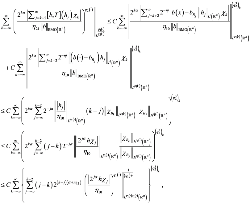
Thus, from Lemmas 3.4-3.7, We obtain that

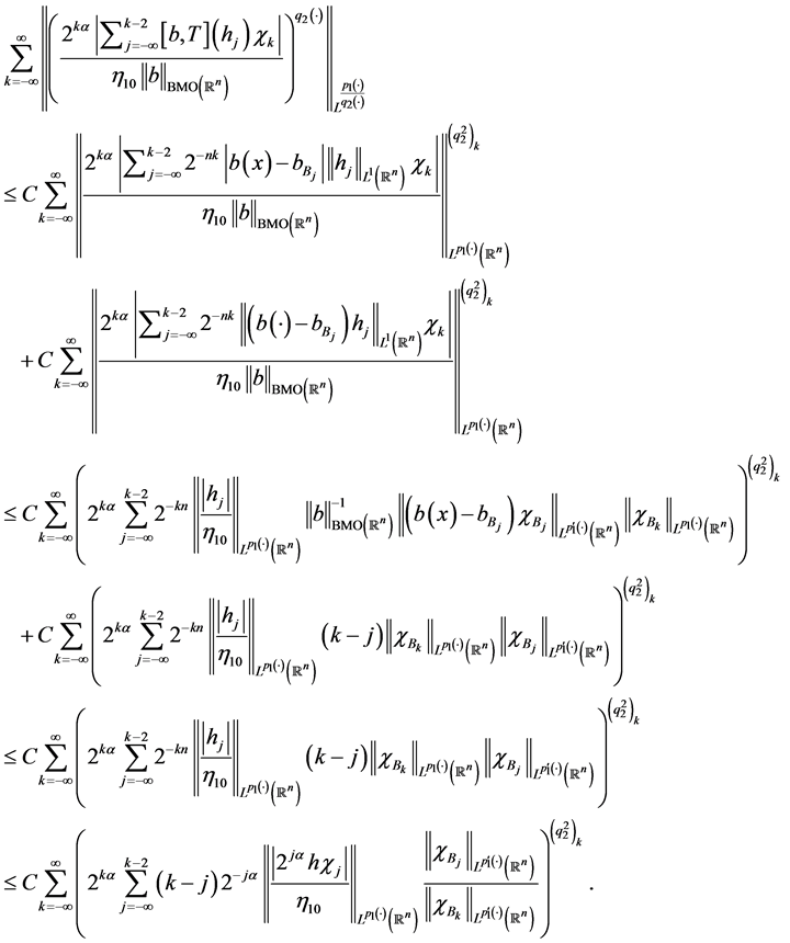
Therefore, we get

$\begin{array}{l}{\displaystyle \underset{k=-\infty }{\overset{\infty }{\sum }}}{\Vert {\left(\frac{2^{k\alpha }\left|{\displaystyle {\sum }_{j=-\infty }^{\infty }\left[b,T\right]\left(h_j\right){\chi }_k}\right|}{{\eta }_{10}{\Vert b\Vert }_{\text{BMO}\left({ℝ}^n\right)}}\right)}^{q_2(\cdot )}\Vert }_{L^{\frac{p_1(\cdot )}{q_2(\cdot )}}}\\ \le C{\displaystyle \underset{k=-\infty }{\overset{\infty }{\sum }}}{\left\{{\displaystyle \underset{j=-\infty }{\overset{k-2}{\sum }}}\left(k-j\right)2^{\left(k-j\right)\left(\alpha -n{\iota }_{11}\right)}{\Vert {\left(\frac{\left|2^{j\alpha }h{\chi }_j\right|}{{\eta }_{10}}\right)}^{q_1(\cdot )}\Vert }_{L^{p_1(\cdot )q_1(\cdot )}\left({ℝ}^n\right)}^{\frac{1}{\left(q_1\right)+}}\right\}}^{{\left(q_2^2\right)}_k},\end{array}$ (4.23)

where

${\left(q_2^2\right)}_k=\{\begin{array}{l}{\left(q_2\right)}_{-},{\Vert {\left(\frac{2^{k\alpha }\left|{\displaystyle {\sum }_{j=-\infty }^{k-2}\left[b,T\right]\left(h_j\right){\chi }_k}\right|}{{\eta }_{10}}\right)}^{q_2(\cdot )}\Vert }_{L^{\frac{p_1(\cdot )}{q_2(\cdot )}}}\le 1,\hfill \\ {\left(q_2\right)}_{+},{\Vert {\left(\frac{2^{k\alpha }\left|{\displaystyle {\sum }_{j=-\infty }^{k-2}\left[b,T\right]\left(h_j\right){\chi }_k}\right|}{{\eta }_{10}}\right)}^{q_2(\cdot )}\Vert }_{L^{\frac{p_1(\cdot )}{q_2(\cdot )}}}>1.\hfill \end{array}$

This, for ${\left(q_1\right)}_{+}<1$ , ${\left(p_1\right)}_{+}\le {\left(p_2\right)}_{-}\le {\left(q_2^2\right)}_k$ , along with Remark 2.2, tells us that

$\begin{array}{l}{\displaystyle \underset{k=-\infty }{\overset{\infty }{\sum }}}{\Vert {\left(\frac{2^{k\alpha }\left|{\displaystyle {\sum }_{j=-\infty }^{k-2}\left[b,T\right]\left(h_j\right){\chi }_k}\right|}{{\eta }_{10}{\Vert b\Vert }_{BMO\left({ℝ}^n\right)}}\right)}^{q_2(\cdot )}\Vert }_{L^{\frac{p_1(\cdot )}{q_2(\cdot )}}}\\ \le C{\left\{{\displaystyle \underset{j=-\infty }{\overset{\infty }{\sum }}}{\Vert {\left(\frac{\left|2^{j\alpha }h{\chi }_j\right|}{{\eta }_{10}}\right)}^{q_1(\cdot )}\Vert }_{L^{p_1(\cdot )q_1(\cdot )}}{\displaystyle \underset{k=j+2}{\overset{\infty }{\sum }}}\left(k-j\right)2^{\left(k-j\right)\left(\alpha -n{\iota }_{11}\right)}\right\}}^{q_{*}}\le C,\end{array}$

where $q_{*}=\underset{k\in N}{\min }\frac{{\left(q_2^2\right)}_k}{{\left(q_1\right)}_{+}}.$

If ${\left(q_1\right)}_{+}\le 1$ , it is follows from Remark 2.2 and Hölder’s inequality that

$\begin{array}{l}{\displaystyle \underset{k=-\infty }{\overset{\infty }{\sum }}}{\Vert {\left(\frac{2^{k\alpha }\left|{\displaystyle {\sum }_{j=-\infty }^{k-2}\left[b,T\right]\left(h_j\right){\chi }_k}\right|}{{\eta }_{10}{\Vert b\Vert }_{\text{BMO}\left({ℝ}^n\right)}}\right)}^{q_2(\cdot )}\Vert }_{L^{\frac{p_1(\cdot )}{q_2(\cdot )}}}\\ \le C{\displaystyle \underset{k=-\infty }{\overset{\infty }{\sum }}}{\left\{{\displaystyle \underset{j=-\infty }{\overset{k-2}{\sum }}}\left(k-j\right)2^{\left(k-j\right)\left(\alpha -n{\iota }_{11}\right){\left(q_1\right)}_{+}/2}{\Vert {\left(\frac{\left|2^{j\alpha }h{\chi }_j\right|}{{\eta }_{10}}\right)}^{q_1(\cdot )}\Vert }_{L^{p_1(\cdot )q_1(\cdot )}}\right\}}^{\frac{{\left(q_2^2\right)}_k}{\left(q_1\right)+}}\\ \times {\left({\displaystyle \underset{j=-\infty }{\overset{k-2}{\sum }}}\left(k-j\right)2^{\left(k-j\right)\left(\alpha -n{\iota }_{11}\right){\left({\left(q_1\right)}_{+}\right)}^{\prime }/2}\right)}^{\frac{{\left(q_2^2\right)}_k}{{\left(\left(q_1\right)+\right)}^{\prime }}}\\ \le C{\left\{{\displaystyle \underset{j=-\infty }{\overset{\infty }{\sum }}}{\Vert {\left(\frac{\left|2^{j\alpha }h{\chi }_j\right|}{{\eta }_{10}}\right)}^{q_1(\cdot )}\Vert }_{L^{p_1(\cdot )q_1(\cdot )}}{\displaystyle \underset{k=j+2}{\overset{\infty }{\sum }}}\left(k-j\right)2^{\left(k-j\right)\left(\alpha -n{\iota }_{11}\right){\left(q_1\right)}_{+}/2}\right\}}^{q_{*}}\\ \le C,\end{array}$

where $q_{*}=\underset{k\in N}{\min }\frac{{\left(q_2^2\right)}_k}{{\left(q_1\right)}_{+}}$ .

This implies that

${\eta }_{21}\le C{\eta }_{10}{\Vert b\Vert }_{\text{BMO}\left({ℝ}^n\right)}\le C{\Vert b\Vert }_{\text{BMO}\left({ℝ}^n\right)}{\Vert h\Vert }_{{\stackrel{\dot{}}{K}}_{p_1(\cdot )}^{\alpha ,q_1(\cdot )}\left({ℝ}^n\right)}.$ (4.24)

Finally we estimate ${\eta }_{23}$ , for any $x\in A_j,\mathrm{<mi>\; </mi>}j\ge k+2$ , by the same way to argument in ${\eta }_{21}$ , we obtain that

$\begin{array}{c}\left|\left[b,T\right]h_j\right|\le {\displaystyle {\int }_{A_j}}\left|K\left(x,y\right)\left(b\left(x\right)-b\left(y\right)\right)h_j\left(y\right)\right|\text{d}y\\ \le C{\displaystyle {\int }_{A_j}}\left|\left(b\left(x\right)-b\left(y\right)\right)h_j\left(y\right)\right|/{\left|x-y\right|}^n\text{d}y\\ \le C{2}^{-nj}\left|b\left(x\right)-b_{B_k}\right|{\displaystyle {\int }_{A_j}}\left|h_j\left(y\right)\right|\text{d}y+{\displaystyle {\int }_{A_j}}\left|b_{B_k}-b\left(y\right)\right|\left|h_j\left(y\right)\right|\text{d}y\\ \le C{2}^{-nj}\left|b\left(x\right)-b_{B_j}\right|{\Vert h_j\Vert }_{L^1\left({ℝ}^n\right)}+{\Vert b(\cdot )-\left(b_{B_j}\right)h_j\Vert }_{L^1\left({ℝ}^n\right)},\end{array}$ (4.25)

and

(4.26)

where

${\left(q_2^3\right)}_k=\{\begin{array}{l}{\left(q_2\right)}_{-},{\Vert {\left(\frac{2^{k\alpha }\left|{\displaystyle {\sum }_{j=-\infty }^{k-2}\left[b,T\right]\left(h_j\right){\chi }_k}\right|}{{\eta }_{10}}\right)}^{q_2(\cdot )}\Vert }_{L^{\frac{p_1(\cdot )}{q_2(\cdot )}}}\le 1,\hfill \\ {\left(q_2\right)}_{+},{\Vert {\left(\frac{2^{k\alpha }\left|{\displaystyle {\sum }_{j=-\infty }^{k-2}\left[b,T\right]\left(h_j\right){\chi }_k}\right|}{{\eta }_{10}}\right)}^{q_2(\cdot )}\Vert }_{L^{\frac{p_1(\cdot )}{q_2(\cdot )}}}>1.\hfill \end{array}$

Hence, we arrive at that ${\eta }_{23}\le C{\eta }_{10}{\Vert b\Vert }_{\text{BMO}\left({ℝ}^n\right)}\le C{\Vert b\Vert }_{\text{BMO}\left({ℝ}^n\right)}{\Vert h\Vert }_{{\stackrel{\dot{}}{K}}_{p_1(\cdot )}^{\alpha ,q_1(\cdot )}\left({ℝ}^n\right)}$ by the similar argument in the proof Theorem 4.1.

This completes the proof of Theorem 4.2. $�$

Acknowledgements

This paper is supported by National Natural Foundation of China (Grant No. 11561062).

References

[1] Calderón, A. and Zygmund, A. (1956) On Singular Integrals. American Journal of Mathematics, 78, 289-309.
[CrossRef]
[2] Calderón, A. and Zygmund, A. (1978) On Singular Integral with Variable Kernels. Applied Analysis, 7, 221-238.
[3] Jouné, J.-L. (1983) Calderón-Zygmund Operators, Pseudo-Differential Operators and the Cauchy Integral of Calderón. In: Lecture Notes in Math, Vol. 994, Springer-Verlag, Berlin, Heidelberg.
[4] Coifman, R., Rochberg, R. and Weiss, G. (1976) Factorization Theorems for Hardy Spaces in Several Variables. Annals of Mathematics, 103, 611-635.
[5] Kovácik, O. and Rákosník, J. (1991) On Spaces Lp(x) and Wk,p(x). Czechoslovak Mathematical Journal, 41, 592-618.
[6] Diening, L. and Ruicka, M. (2003) Calderón-Zygmund Operators on Generalized Lebesgue Spaces Lp(.) and Problems Related to Fluid Dynamics. Journal für die Reine und Angewandte Mathematik, 563, 197-220.
[7] Chen, Y., Levine, S. and Rao, M. (2006) Variable Exponent, Linear Growth Functionals in Image Restoration. SIAM Journal on Applied Mathematics, 66, 1383-1406.
[8] Li, F., Li, Z. and Pi, L. (2010) Variable Exponent Functionals in Image Restoration. Applied Mathematics and Computation, 216, 870-882.
[9] Harjulehto, P., Hasto, P., Latvala, V. and Toivanen, O. (2013) Critical Variable Exponent Functionals in Image Restoration. Applied Mathematics Letters, 26, 56-60.
[10] Izuki, M. (2009) Herz and Amalgam Spaces with Variable Exponent, the Haar Wavelets and Greediness of the Wavelet System. East Journal on Approximations, 15, 87-109.
[11] Izuki, M. (2010) Boundedness of Commutators on Herz Spaces with Variable Exponent. Rendiconti del Circolo Matematico di Palermo, 59, 199-213.
[12] Izuki, M. (2010) Fractional Integrals on Herz-Morrey Spaces with Variable Exponent. Hiroshima Mathematical Journal, 40, 343-355.
[13] Wang, L. and Tao, S. (2014) Boundedness of Littlewood-Paley Operators and Their Commutators on Herz-Morrey Spaces with Variable Exponent. Journal of Inequalities and Applications, 2014, 227.
[14] Wang, L. and Tao, S. (2015) Parameterized Littlewood-Paley Operators and Their Commutators on Lebegue Spaces with Variable Exponent. Analysis in Theory and Applications, 31, 13-24.
[15] Tan, J. and Liu, Z. (2015) Some Boundedness of Homogeneous Fractional Integrals on Variable Exponent Function Spaces. ACTA Mathematics Science (Chinese Series), 58, 310-320.
[16] Omer, A., Afif, A. and Tao, S. (2016) The Boundedness for Commutators of Calderón-Zygmund Operator on Herz-Tybe Hardy Spaces with Variable Exponent. Journal of Applied Mathematics and Physics, 4, 1157-1167.
[17] Wang, L. and Tao, S. (2016) Parameterized Littlewood-Paley Operators and Their Commutators on Herz Spaces with Variable Exponents. Turkish Journal of Mathematics, 40, 122-145.
[18] Cuz-Uribe, D., Fiorenza, A., Martell, J.M. and Perez, C. (2006) The Boundedness of Classical Operators on Variable Lp Spaces. Annales Academiae Scientiarum Fennicae-Mathematica, 31, 239-264.
[19] Almeida, A., Hasanov, J. and Samko, S. (2008) Maximal and Potential Operators in Variable Exponent Morrey Spaces. Georgian Mathematical Journal, 15, 195-208.
[20] Cruz-Uribe, D. and Fiorenza, A. (2013) Variable Lebesgue Spaces: Foundations and Harmonic Analysis. In: Applied and Numerical Harmonic Analysis, Springer, New York.
[21] Diening, L. (2005) Maximal Function on Musielak-Orlicz Spaces and Generalized Lebesgue Spaces. Bulletin des Sciences Mathématiques, 129, 657-700.
Copyright © 2026 by authors and Scientific Research Publishing Inc.
Creative Commons License
This work and the related PDF file are licensed under a Creative Commons Attribution 4.0 International License.