Ilhan M. Izmirli
George Mason University, Fairfax, USA.
DOI: 10.4236/am.2015.66101   PDF    HTML   XML   6,353 Downloads   7,852 Views   Citations

Abstract

The Pascal matrix and the Fibonacci matrix are among the most well-known and the most widely-used tools in elementary algebra. In this paper, after a brief introduction where we give the basic definitions and the historical backgrounds of these concepts, we propose an algorithm that will generate the elements of these matrices. In fact, we will show that the indicated algorithm can be used to construct the elements of any power series matrix generated by any polynomial (see Definition 1), and hence, it is a generalization of the specific algorithms that give us the Pascal and the Fibonacci matrices.

Keywords

Pascal Triangle, Fibonacci Triangle

Share and Cite:

1. Introduction

1.1. Pascal’s Triangle and Pascal’s Matrix

The binomial formula

where the binomial coefficients can easily be computed using the addition rule

for any two non-negative integers and with, is one of the most well-known formulas in elementary algebra.

It is customary to call the triangular array made up of the binomial coefficients

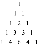
the Pascal’s triangle. This triangle has some simple yet interesting properties that are familiar to most introductory algebra students:

i) Horizontal rows add to powers of 2, which can, of course, easily be shown by putting in the binomial formula.

ii) The horizontal rows represent powers of 11, which can, of course, easily be shown by putting a = 10 and b = 1 in the binomial formula.

iii) Adding any two successive numbers in the diagonal containing the triangular numbers results in a perfect square. This, of course, is a direct consequence of the definition of triangular numbers. The

triangular number is. So the sum of two consecutive triangular numbers is

iv) In the expansion of, where is a prime number, all coefficients that are greater than 1 are divisible by; that is, if the first number to the right of 1 in any row is a prime number, then all numbers greater than 1 in that row are divisible by that prime number.

Any coefficient is of the form. If p is prime, then, by definition, and are factors of

. Therefore, since p cannot possibly be in the denominator, some multiple of p must be left in the numerator, making the coefficient an integer which is a multiple of p.

It is now acknowledged that this triangle was known well before Blaise Pascal (1623-1662) who “introduced” it in his famous 1653 treatise, Traité du triangle arithmétique. Indeed, not only the binomial coefficients, but in fact, the addition rule, which, of course, is needed to generate the coefficients, were known to Indian mathematicians¹. For instance, according to Edwards [1] , some elements of the binomial coefficients can be observed in the works of Pingala (c. 200 BC-?). A few centuries later, Varahamihira (505 CE-587 CE) gave a clear description of the addition rule [1] 2013). The triangle itself was mentioned as early as the 10^th century CE, in the book Meru-prastaara² by Halayudha (?-?). See [2] for more details.

Persian mathematicians were also well acquainted with the binomial coefficients―this can be seen, for example, in the writings of Al-Karaji (953-1029) and later in those of Omar Hayyam (1048-1131), who indeed set up the entire triangle. Thus, some scholars and historians refer to the triangle as the Khayyam-Pascal triangle (see [3] ).

Many other cultures were familiar with the triangle and its properties as well. For example, the triangle was known in China in the early 11^th century, a fact that is, according to [4] , corroborated by the works of the Jia Xian (1010-1070) and Yang Hui (1238-1298).

There were also precedents in the west. The German humanist, Petrus Apianus (1495-1552), known for his works in mathematics, astronomy, and cartography, published the full triangle in 1527. In the second half of 16^th century, parts of the triangle were published by the German monk and mathematician Michael Stifel (1487- 1567), and the Italian mathematicians Niccolo Fontana Tartaglia (1499-1557) and Gerolamo Cardano (1501- 1576) See [3] foe more details.

A closely related idea is that of the Pascal matrix. The Pascal matrix is an infinite matrix containing the Pascal triangle as a submatrix. There are three convenient ways of doing this:

a) As a lower triangular matrix where the binomial coefficients are placed in rows. For example,

b) As an upper triangular matrix where the binomial coefficients are placed in columns. For example,

c) As a symmetric matrix where the binomial coefficients are placed on the subdiagonals. For example,

See [5] for more information on Pascal matrices.

Clearly, In fact, it can be shown that and consequently,

See [6] for a proof.

1.2. The Fibonacci Triangle

As is well-known, the Fibonacci sequence, is defined recursively as

and for,

The sequence is named after Leonardo of Pisa (Fibonacci) (c.1170-c. 1250), who in his 1202 book Liber Abaci introduced it to the European readers. However, as was the case with Pascal’s triangle, this sequence had been described earlier by Indian mathematicians as well. See [7] or [8] for more information.

The Fibonacci triangle is a two-dimensional version of the Fibonacci sequence. It is defined as follows:

For

and for

So this is a triangle with Fibonacci sequences on the sides. Note that the subdiagonals are Fibonacci sequences as well, except that the starting value is no longer . So, the left edge of the triangle (as well as the right edge) is the Fibonacci sequence, the diagonal parallel to it is the Fibonacci sequence, the next diagonal is the Fibonacci sequence starting with, the next is the Fibonacci sequence starting with, the next a Fibonacci sequence starting with, and so on.

See [9] for more details.

2. The Connection between the Pascal and Fibonacci Matrices and Power Series

It is easy to see that if we let

for, then the coefficients in the power series of

arranged in a matrix gives us the Pascal matrix. For,

If we now form a matrix where the row consists of the coefficients of the power series of, for

, we get the Pascal matrix:

It is now natural to ask the following question: If, is replaced by some arbitrary polynomial of degree and the same process is applied, what types of matrices will we get?

Definition 1. Let with and. Let stand for the coefficient of

in the power series expansion of,;. Then, the infinite matrix

whose entry is will be called the power series matrix generated by.

Example 1. The simplest example is For,

So, the power series matrix generated by would be

Example 2. As another example let us consider the function. Indeed, multiplying both sides of

by, we obtain

implying

and

for. Hence,

To find power series expansions of we note that for any

Hence, differentiating both sides of the identity for and multiplying by the power series of we obtain

Similarly,

and so on. Consequently,

Hence, the power series matrix generated by, is the Fibonacci matrix.

3. The Algorithm

Now we want to give an algorithm that will give us the entries of more rapidly. Let

with and. Let stand for the coefficient of in the power

series expansion of,

Set

and if, set

Now for

and

For

and

To see why this algorithm works, for, let us set

Note that the coefficient of in the product

is.

Consequently, for

Since

we have for

This algorithm is, of course, a natural generalization of the addition process we apply to calculate various coefficients in Pascal’s triangle. In fact, in case, our algorithm simply becomes

Examples:

1) The power series matrix of is

2) The power series matrix of is

NOTES

¹However, keeping up with “tradition,” we will, throughout this paper, refer to the triangle as Pascal’s triangle.

²This title translates as The Staircase of Mount Meru.

Conflicts of Interest

The authors declare no conflicts of interest.

References

[1]	Edwards, A.W.F. (2002) Pascal’s Arithmetical Triangle: The Story of a Mathematical Idea. John Hopkins University Press, Baltimore.
[2]	Edwards, A.W.F. (2013) The Arithmetical Triangle. In: Wilson, R. and Watkins, J.J., Eds., Combinatorics: Ancient and Modern, Oxford University Press, Oxford, 166-180. http://dx.doi.org/10.1093/acprof:oso/9780199656592.003.0008[CrossRef]
[3]	Coolidge, J.L. (1949) The Story of the Binomial Theorem. The American Mathematical Monthly, 56, 147-157. http://dx.doi.org/10.2307/2305028[CrossRef]
[4]	Smith, K.J. (2010) Nature of Mathematics, Cengage Learning.
[5]	Call, G.S. and Velleman, D.J. (1993) Pascal’s Matrices. American Mathematical Monthly, 100, 372-376. http://dx.doi.org/10.2307/2324960[CrossRef]
[6]	Alan, E. and Strang, G. (2004) Pascal Matrices. American Mathematical Monthly, 111, 361-385.
[7]	Goonatilake, S. (1998) Toward a Global Sciece. Indiana University Press, Bloomington.
[8]	Siegler, L.E. (2002) Fibonacci’s Liber Abaci: A Translation into Modern English of the Book of Calculation, Sources and Studies in the History of Mathematics and Physical Sciences. Springer, Berlin. http://dx.doi.org/10.1007/978-1-4613-0079-3[CrossRef]
[9]	Hoggartt Jr., V.E. and Bricknell, M. (1974) Triangular Numbers. The Fibonacci Quarterly, 12, 221-230.