Qibo Luo, Dong Han^*
School of Mechanical Engineering, University of Shanghai for Science and Technology, Shanghai, China.
DOI: 10.4236/jpee.2026.143005   PDF    HTML   XML   72 Downloads   267 Views   Citations

Abstract

As the low carbon transition of power systems accelerates, low carbon demand response, characterized by both environmental orientation and behavioral incentives, has become a key mechanism for enhancing grid flexibility and an important collaborative approach for optimizing carbon emissions. This paper proposes an optimization strategy for customer directrix load based demand response founded on an electricity carbon incentive cross elasticity matrix. First, a similarity evaluation metric is constructed based on actual response contributions to assess the effectiveness of users’ direct participation in customer directrix load demand response. At the same time, an actual response volume metric is introduced to quantify response contributions, forming a comprehensive response indicator. On this basis, a segmented incentive price function is designed to more fairly reflect the response contributions of different users. Second, differentiated penalty factors are incorporated into the incentive price function according to the temporal scale of varying carbon emission levels. This approach establishes an incentive cross elasticity matrix that incorporates users’ low carbon behaviors, thereby encouraging load curve adjustments while promoting low carbon electricity consumption. Finally, an optimization model for load curve based low carbon demand response is developed with the objective of minimizing users’ total energy costs under constraints including response capacity limits and electricity balance. The results demonstrate that the proposed strategy effectively guides users to proactively adjust their electricity consumption behavior. It reduces overall costs while suppressing peak valley differences and optimizing carbon emissions, highlighting synergistic advantages in economic efficiency, low carbon performance, and controllable response behavior.

Keywords

Customer Directrix Load, Low-Carbon Demand Response, Dynamic Carbon Emission Factor, Cross-Elasticity Matrix

Share and Cite:

1. Introduction

The power sector is a major contributor to carbon emissions. Promoting the low-carbon transformation of power systems holds significant strategic importance for optimizing the energy structure and achieving sustainable development of the power grid. With the advancement of large-scale distributed energy resources (DERs) and information and communication technologies, prosumers can now share energy at the distribution grid level. Prosumers can not only supply surplus energy to other users through market-based mechanisms but also actively participate in system energy regulation via distributed resources. Against this backdrop, Demand Response (DR) serves as a key mechanism linking flexible resources on the consumer side with system operational objectives, leveraging the regulatory capacity of flexible demand-side resources to enhance grid flexibility.

Demand response primarily falls into two categories: price-based and incentive-based. The incentive-based approach includes methods such as interruptible load, direct load control, and peak subsidies. Compared to price-based mechanisms, incentive-based approaches do not involve electricity price adjustments, cause minimal market disruption, and incur no actual losses for users, thereby facilitating broader participation. Currently, incentive-based DR widely employs customer baseline load (CBL) to evaluate user response contributions [1]. To enhance the accuracy of response effectiveness assessments, extensive research has focused on precise CBL calculation methods. Examples include CBL prediction methods integrating K-means with long short-term memory (LSTM) neural networks [2], and the use of virtual control groups [3]. While these approaches have improved response evaluation accuracy to some extent, CBL fundamentally relies on historical load data. This makes it difficult to completely prevent users from engaging in strategic behaviors on non-response days, such as deliberately increasing electricity consumption to artificially inflate the baseline—thereby obtaining inflated load reduction figures and unjustified incentive compensation on response days. To mitigate this risk and enhance the fairness and effectiveness of demand response, reference [4] proposed Customer Directrix Line (CDL) demand response (hereafter referred to as Directrix-based DR). Directrix-based DR combines self-optimization mechanisms to incentivize users to independently optimize their electricity consumption patterns, thereby coordinating fluctuations between flexible resources and inflexible loads to achieve grid operators’ control objectives. It exhibits four key characteristics: simplified management, clear objectives, broad adaptability, and sustainable response [5], overcoming limitations of traditional response methods such as difficulty in routine implementation and restricted participation scale. Existing research primarily focuses on system economics or load adjustability as optimization objectives, emphasizing renewable energy integration [6], regional benefit enhancement [7], or strengthening system flexibility and responsiveness [8]. Regarding incentive mechanism design, scholars have introduced comprehensive evaluation metrics based on response proactivity and contribution, alongside differentiated incentive strategies, to boost participation willingness and response effectiveness among small and medium-sized users [9].

Concurrently, acknowledging users’ inherent bounded rationality [10], existing studies have applied behavioral economics theories to characterize response mechanisms. Reference [11] modeled users’ subjective perceptions of price distributions using probability weighting functions, demonstrating the feasibility of intervening in irrational behaviors. Reference [12] revealed the guiding role of pricing mechanisms on user load behaviors. while reference [13] further explores optimizing demand response strategies through behavioral preferences, risk perception, and acceptance thresholds to boost user participation. As increasing research focuses on low-carbon demand response mechanisms, positive progress has been made in incentive design, user behavior modeling, and multi-energy system coordination, propelling demand response toward low-carbon and refined approaches. Therefore, there is an urgent need to establish an incentive mechanism that encourages users to voluntarily shift their energy consumption from high-carbon emission periods to low-carbon emission periods. Existing incentive mechanisms mostly focus on price optimization for a single period, neglecting the behavioral coupling effects triggered by incentives across multiple periods. When users respond to incentives in one period, they often alter their electricity usage patterns in other periods, leading to cross-period linkage behaviors. To address this, this paper proposes establishing an incentive cross-elasticity matrix that captures users’ low-carbon behaviors. Differentiated incentive prices are set for periods with varying carbon emission intensities, enabling effective modeling of users’ low-carbon response behaviors. This approach optimizes quasi-linear demand response strategies across all periods.

In summary, this paper introduces dynamic carbon emission factors into a customer directrix load demand response mechanism. First, a segmented incentive price function is constructed based on a comprehensive evaluation metric combining user response similarity and actual adjustment contribution. By integrating carbon emission intensity differences across time periods with incentive linkage effects, an electricity-carbon incentive cross-elasticity matrix is established to achieve precise modeling and guidance of response behavior, thereby optimizing incentive strategies for all time periods. Second, a quasi-linear low-carbon demand response optimization model is formulated, targeting the minimization of users’ comprehensive energy costs. Finally, three simulation scenarios are designed to validate the effectiveness and feasibility of the proposed model.

2. Customer Directrix Load-Based Demand Response Mechanism

Figure 1 presents the overall framework of the load-based low-carbon demand response mechanism proposed in this paper. This mechanism primarily involves two types of entities: power grid companies and users equipped with distributed energy resources. On the consumer side, users deploy distributed photovoltaic systems, micro-gas turbines, and energy storage devices, functioning as prosumers capable of both generating and consuming energy. These users can share energy and exchange information with one another. Based on forecasted uncontrollable loads, renewable generation output, and other data, the grid operator calculates the customer directrix load curve and dynamic carbon emission factor curve, then disseminates incentive price signals to the user side. Guided by the published load reference curve and corresponding incentive prices, users adjust their energy consumption behavior to minimize their comprehensive energy costs. Consequently, it guides users to rationally adjust their energy consumption timing while responding to the customer directrix load curve, achieving coordinated regulation of load tracking and carbon emission optimization.

Figure 1. Framework of CDL-based low carbon DR.

3. Method for Constructing Cross-Elasticity Matrix of Electricity-Carbon Incentives on the User Side

3.1. Customer Directrix Load-Based Demand Response

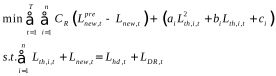
The customer directrix load curve serves as a benchmark load profile to smooth fluctuations caused by non-dispatchable generation resources and loads within the power grid. It is established by the grid operator based on regulation requirements. Users proactively adjust their energy consumption strategies by receiving published load reference curve and incentive price signals of grid operator, aiming to align their load profiles as closely as possible with the reference curve shape to earn corresponding incentive rewards. The customer directrix load curve is derived by inverting the net load curve after deducting renewable energy output and adopting the shape of its envelope. Its model is shown in Equation (1), where the first term of the objective function represents the total operating cost of thermal power units, and the second term reflects the penalty cost for curtailed wind and solar power. The constraint condition is the power balance constraint.

(1)

where, $a_i^{}$ , $b_i^{}$ and $c_i^{}$ are the cost coefficients for thermal power unit i. $L_{th,i,t}^{}$ is the power output of thermal power unit i at time t. $C_R^{}$ is the wind and solar curtailment cost coefficient. $L_{new,t}^{pre}$ is the predicted value of new energy generation power at time t. $L_{new,t}^{}$ is the output power of the new energy source at time t. $L_{hd,t}^{}$ is the non-adjustable load power at time t. $L_{DR,t}^{}$ is the customer directrix load value at time t.

First, the shape of the load curve must be defined, where $L_t$ denotes the daily load curve and ${\displaystyle {\sum }_{t=1}^T{L}_t}$ represents the total electricity consumption within a day. By normalizing the load curve with respect to total electricity consumption, a normalized daily load curve is obtained, expressed as:

(2)

where, $Q_t$ is the normalized load of users during time period t. The customer directrix load is a normalized signal that preserves only shape characteristics, serving as a load shaping target for all demand response participants.

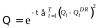
By quantifying the similarity between user response load curves and load reference lines (hereinafter referred to as user response similarity), targeted incentive schemes are formulated. The formula for user response similarity is:

(3)

where, $\tau$ is the response sensitivity coefficient, which controls the extent to which the distance between the load curve and the load reference line affects the response effect measurement $\Theta$ . $Q_t^{DR}$ is the normalized load reference line value for time period t. The response sensitivity coefficient $\Theta$ is introduced to regulate the discrimination strength of the similarity evaluation. In this study, $\Theta$ is determined through heuristic calibration based on preliminary simulations, ensuring that deviations between the user load curve and the customer directrix load are sufficiently distinguished without excessively amplifying minor fluctuations. This parameter can also be calibrated using historical demand response data or operator experience in practical applications.

To fairly evaluate user response, this paper further defines the user response contribution metric $\Xi$ , which quantifies the ratio between the actual load adjustment amount and the maximum adjustable capacity of users.

$\Xi =\frac{{\displaystyle \sum _{t=1}^T\left|\Delta L_{n,t}\right|}}{{\displaystyle \sum _{t=1}^T\Delta L_{n,t}^{\max }}}$ (4)

where, $\Delta L_{n,t}$ is the difference between the original load power of user n and the load power of user n after demand response. $\Delta L_{n,t}^{\max }$ is the maximum adjustable load capacity for user n during time period t. The value range of $\Xi$ is [0, 1]. The higher the value, the greater the proportion of adjustable potential the user has utilized to participate in the response, indicating a more significant actual contribution.

To balance response accuracy (i.e., user response similarity) and response intensity (i.e., actual adjustment contribution), this paper proposes a comprehensive response index as the final basis for users to obtain incentives.

$\Pi =\epsilon \Theta +\left(1-\epsilon \right)\Xi$ (5)

where, $\epsilon$ is the weighting coefficient used to adjust the relative importance of similarity and contribution in the comprehensive evaluation. When a user’s comprehensive response metric falls below ${\Pi }_0$ , the incentive price is 0, when a user’s comprehensive response metric exceeds ${\Pi }_m$ , the their response incentive price reaches the maximum value $I_{\max }$ . Where, $\epsilon$ is the weighting coefficient used to balance the relative importance of response similarity and actual adjustment contribution in the comprehensive evaluation. In this paper, $\epsilon$ is selected to reflect a trade-off between response accuracy and response intensity, and its value is determined through comparative simulation to avoid overemphasizing either curve-shape matching or adjustment magnitude. In practice, $\epsilon$ can be flexibly adjusted according to operator policy preferences or different demand response program objectives.

To encourage users to actively participate in load-based demand response, the segmented incentive pricing function designed in this paper is illustrated in Figure 2. This mechanism allocates rewards based on users’ comprehensive response performance. Both the similarity of user responses and the actual adjustment contribution jointly determine the comprehensive response performance; the higher the value of $\Pi$ , the greater the incentive level received.

Figure 2. Segmented incentive price function of user.

3.2. Electrical-Carbon Cross-Elasticity Matrix

To ensure fairness in user responses and facilitate unified management, the daily dynamic average carbon emission factor is calculated using the proportion of non-clean energy supply within a specific regional system, with a time scale of 1 hour. The specific calculation is as follows:

(6)

where, ${\alpha }_{\text{CF},t}$ is the dynamic carbon emission factor. ${\alpha }_{th,i}$ is the carbon emission intensity of thermal power unit i in this region. $L_{th,i,t}$ is the net output of the thermal power unit i during time period t. $L_{g,W,t}^{}$ and $L_{g,PV,t}^{}$ are the grid-connected power output of wind power and solar power, respectively, within the region during time period t. $L_{j,t}$ is the electrical power delivered to region j from region i during time interval t. ${\alpha }_{j,t}$ is the carbon emission intensity for region j during time period t. The dynamic carbon emission factor adopted in this paper represents an hourly average carbon emission intensity of the regional power system. It is calculated based on the generation mix, including thermal power generation, renewable energy outputs, and inter-regional power exchanges. The factor reflects average emissions rather than marginal emissions, which is suitable for incentive-based demand response programs aiming to guide users toward low-carbon electricity consumption patterns.

Carbon emission periods are categorized into high-peak and low-trough segments based on regional dynamic emission factors, with fuzzy membership functions applied for analysis. Membership indices serve as the evaluation criteria, dividing periods into carbon peak period membership $f_t$ and carbon trough period membership $g_t$ .

$f_t=\frac{x-{\alpha }_{CF,t}}{x-y}$ (7)

$g_t=\frac{{\alpha }_{CF,t}-y}{x-y}$ (8)

where, x represents the maximum dynamic carbon emission factor; y represents the minimum dynamic carbon emission factor. ${\alpha }_{CF,t}$ is the dynamic carbon emission factor during time period t.

In the incentive pricing reward and penalty mechanism based on dynamic carbon emission factors, electricity consumption periods are categorized into high-carbon, flat-carbon, and low-carbon periods according to these factors. Incentive prices are reduced during high-carbon periods, increased during low-carbon periods, and maintained at the original level during medium-carbon periods, as shown in Formula (10). Through differentiated incentive pricing, users are guided to shift transferable loads from high-carbon emission periods to low-carbon emission periods in an orderly manner, subject to the premise of optimizing overall energy consumption costs. This achieves an optimized temporal distribution of carbon emissions.

${\overline{\alpha }}_{\text{CF},t}=\frac{{\alpha }_{\text{CF},t}-A}{B-A}$(9)

$I_{n,t}^{*}=\{\begin{array}{l}\left(1-{\overline{\alpha }}_{\text{CF},t}\right)I_{n,t}^{}\text{, }t\in T_{high}^{}\\ I_{n,t}^{}\text{, }t\in T_{average}^{}\\ \left(1+{\overline{\alpha }}_{\text{CF},t}\right)I_{n,t}^{}\text{, }t\in T_{low}^{}\end{array}$(10)

where, $I_{n,t}^{}$ is the original demand response incentive price for user n during time period t. $I_{n,t}^{*}$ is the adjusted demand response incentive price. ${\overline{\alpha }}_{\text{CF},t}$ is the dimensionless dynamic carbon emission factor, serving as the penalty factor for the incentive price. $A$ is the minimum dynamic carbon emission factor within a 24-hour period. $B$ is represents the maximum dynamic carbon emission factor within a 24-hour period. $T_{high}^{}$ , $T_{average}^{}$ and $T_{low}^{}$ denote high-carbon, flat-carbon, and low-carbon periods, respectively.

Users alter their original electricity consumption patterns and methods in response to changes in incentive pricing. The elasticity coefficient η represents the sensitivity of electricity consumption during different time periods to incentive pricing, expressed as:

$\varsigma =\frac{\Delta L/L}{\Delta I/I}$ (11)

where, $\Delta L$ is the change in electricity consumption. $L$ is the electricity consumption prior to the change. $\Delta I$ is the change in incentive pricing. $I$ is the incentive pricing prior to the change.

Users decide whether to reduce or shift their load based on the dynamic incentive price signals released by the power grid company, while considering their own response costs and expected benefits. The expression for the incentive price elasticity matrix M is:

${\rm M}=\left(\begin{array}{ccc}{\varsigma }_{hh}& {\varsigma }_{ha}& {\varsigma }_{hl}\\ {\varsigma }_{ah}& {\varsigma }_{aa}& {\varsigma }_{al}\\ {\varsigma }_{lh}& {\varsigma }_{la}& {\varsigma }_{ll}\end{array}\right)$ (12)

where, ${\varsigma }_{hh}$ , ${\varsigma }_{aa}$ and ${\varsigma }_{ll}$ are the auto-elasticity coefficients of user electricity consumption and incentive prices during high-carbon, medium-carbon, and low-carbon periods, respectively. The remaining coefficients are cross-elasticity coefficients. The cross-elasticity coefficients are constructed to reflect users’ load-shifting behavior across different carbon emission periods. In order to ensure behavioral consistency, these coefficients are constrained to be negative, indicating that an increase in incentive price in one period leads to load reduction in that period and corresponding load transfer to other periods. In addition, the magnitude of cross-elasticity coefficients is bounded to avoid unrealistic load migration and to maintain overall energy conservation across periods. In practical applications, these coefficients can be estimated using historical demand response data or survey-based elasticity studies.

For multi-period demand response, the expressions for electricity consumption during high-carbon, medium-carbon, and low-carbon periods are as follows:

$L_{DR}=L_{or}+\left(\begin{array}{ccc}{L}_{or,h}& 0& 0\\ 0& L_{or,a}& 0\\ 0& 0& L_{or,l}\end{array}\right)M\left(\begin{array}{c}\Delta I_h/I_{o,h}\\ \Delta I_a/I_{o,a}^{}\\ \Delta I_l/I_{o,l}^{}\end{array}\right)$ (13)

where, $L_{or,h}$ , $L_{or,a}$ and $L_{or,l}$ are electricity consumption during high-carbon, medium-carbon, and low-carbon periods respectively prior to demand response. $I_{o,h}$ , $I_{o,a}$ and $I_{o,l}$ are the segmented incentive prices before adjustment for high-carbon, medium-carbon, and low-carbon periods, respectively. $\Delta I_h$ , $\Delta I_a$ and $\Delta I_l$ the incentive price differentials after demand response. $L_o$ and $L_{DR}$ are the electricity consumption during the respective periods before and after the demand response.

4. An Optimal Customer Directrix Load-Based Low-Carbon Demand Response Model Based on the Cross-Elasticity Matrix of Electricity-Carbon Incentives

4.1. Objective Function

The objective function of the optimization model is to minimize the user’s comprehensive energy consumption cost, with the specific formula as follows:

$\min F_n=F_{grid,n}^{ele}+F_{P2P,n}^{ele}+F_n^{comf}+F_n^{ca}+F_n^{MT}+F_n^{ESS}-B_n^{DR}$ (14)

where, $B_n^{DR}$ is the revenue for user n participating in demand response. $F_{grid,n}^{ele}$ is electricity transaction costs. $F_{P2P,n}^{ele}$ is peer-to-peer transaction costs. $F_n^{comf}$ is user comfort costs. $F_n^{ca}$ is user carbon emission costs. $F_n^{MT}$ is the power generation cost of micro gas turbines. $F_n^{ESS}$ is battery degradation costs.

$B_n^{DR}={\displaystyle \sum _{t=1}^T{\displaystyle \sum _{n=1}^N{I}_{n,t}^{*}{L}_{n,t}^{adj}}}$ (15)

where, $L_{n,t}^{adj}$ is the total adjustable energy for user n at time t.

$F_{grid,n}^{ele}={\displaystyle \sum _{t=1}^T\left(F_{buy,m,t}^{}-B_{sell,m,t}^{}\right)}$ (16)

$F_{buy,n,t}^{}=r_{buy,t}{L}_{buy,n,t}^{}$ (17)

$B_{sell,n,t}^{}=r_{sell,t}{L}_{sell,n,t}^{}$ (18)

where, $F_{sell,m,t}^{}$ and $B_{buy,m,t}^{}$ are electricity sales revenue and purchase costs of user n during time period t. $r_{buy,t}^{}$ and $r_{sell,t}^{}$ are the prices at which user n purchases and sells electricity to the grid during time period t. $L_{buy,n,t}^{}$ is the electricity purchased from the grid during time period t. $L_{sell,n,t}^{}$ and $L_{buy,n,t}^{}$ are the electricity purchased from and sold to the grid during time period t.

$F_{P2P,n}^{ele}={\displaystyle \sum _{t=1}^{\text{T}}{r}_{n,t}{L}_{P2P,n,t}^{}}={\displaystyle \sum _{t=1}^{\text{T}}{\displaystyle \sum _{k\in N/n}^{}{r}_{n,t}{L}_{P2P,t}^{k\to n}}}$ (19)

where, $r_{n,t}$ is the P2P transaction price for user n during time period t, and $r_{n,t}$ lies between the price at which electricity is sold to the grid and the price at which electricity is purchased from the grid. $L_{P2P,n,t}^{}$ is the total electricity purchased by user n from other users at time t. $L_{P2P,t}^{k\to n}$ is the transaction power from user k to user n.

Any deviation from the preferred load inevitably incurs user load costs. These costs are described using a quadratic function, expressed as follows:

$F_n^{comf}={\displaystyle \sum _{t=1}^T\left[\frac{1}{2}{\lambda }_n\Delta L_{n,t}{}^2\right]}$ (20)

where, ${\lambda }_n$ is the rejection cost coefficient for user n’s participation in demand response.

$F_n^{ca}=r_{ca}{\displaystyle \sum _{t=1}^T{e}_t{L}_{n,t}^{DR}}$ (21)

where, $r_{ca}$ is the unit carbon emission cost. $e_t$ is the carbon emission intensity during time period t. $L_{n,t}^{DR}$ is the electricity load of user n during time period t following demand response.

$F_n^{ESS}={\displaystyle \sum _{t=1}^T{r}_n^{ESS}\left(L_{ch,n,t}^{ESS}+L_{dis,n,t}^{ESS}\right)}$ (22)

where, $r_n^{ESS}$ is the unit cost of battery degradation. $L_{dis,n,t}^{ESS}$ and $L_{ch,n,t}^{ESS}$ are the discharge power and charge power of user n’s energy storage device at time t, respectively.

$F_n^{MT}={\displaystyle \sum _{t=1}^T\left(a_n^{MT}{\left(L_{n,t}^{MT}\right)}^2+b_n^{MT}{L}_{n,t}^{MT}+c_n^{MT}\right)}$ (23)

where, $a_n^{MT}$ , $b_n^{MT}$ and $c_n^{MT}$ are the cost coefficients for user n’s micro gas turbine. $L_{n,t}^{MT}$ is the power output of user n’s micro gas turbine.

4.2. Constraints

The power balance constraint ensures that the total power generation and load demand remain in real-time equilibrium.

$L_{buy,n,t}^{}+L_{n,t}^{PV}+L_{n,t}^{MT}+L_{dis,n,t}^{ESS}+L_{n,t}^{P2P}-L_{ch,n,t}^{ESS}-L_{sell,n,t}^{}=L_{n,t}^{\text{DR}}$ (24)

When participating in demand response, users should meet their own minimum electricity needs while alleviating the pressure on their daily life and production electricity arrangements.

$0\le \left|L_{n,t}^o-L_{n,t}^{DR}\right|\le \Delta L_{n,t}^{\max }$ (25)

where, $L_{n,t}^o$ is the original load power of user n. $L_{n,t}^{DR}$ is the load power after demand response of user n. $\Delta L_{n,t}^{\max }$ is the maximum response volume for user n during time period t.

User participation in demand response must satisfy power balance constraints to ensure that total electricity consumption remains constant throughout the dispatch cycle.

${\displaystyle \sum _{t=1}^T\left(L_{n,t}^o-L_{n,t}^{DR}\right)}=0$ (26)

Transactions between users utilizing surplus electricity can reduce their electricity costs. Considering the actual transmission capacity of power lines, constraints must also be imposed on the transaction volume between users:

$L_{P2P,t}^{k\to n}+L_{P2P,t}^{n\to k}=0$ (27)

$-L_{P2P,\max }^{}\le L_{P2P,t}^{k\to n}\le L_{P2P,\max }^{}$ (28)

where, $L_{P2P,\max }^{}$ is the upper limit of actual line transmission power under secure operation.

User-deployed distributed photovoltaic power generation systems enable self-generation and self-consumption of electricity, while converting surplus generation into economic value through peer-to-peer (P2P) transactions or net metering mechanisms. Given the near-zero marginal cost characteristic of photovoltaic power generation, the operational model established in this paper can be expressed as:

$0\le L_{n,t}^{PV}\le L_{pv,n,t}^{\max }$ (29)

where, $L_{n,t}^{PV}$ is the photovoltaic power generation output for user n at time t. $L_{pv,n,t}^{\max }$ is the maximum output capacity of distributed photovoltaic system of user n.

Micro Turbines (MT) serve as backup power sources for users. During operation, MTs must meet output upper and lower limit constraints as well as ramping constraints.

$L_{MT,m}^{\min }\le L_{n,t}^{MT}\le L_{MT,m}^{\max }$ (30)

$D_n\Delta t\le L_{n,t}^{MT}-L_{n,t-1}^{MT}\le U_n\Delta t$ (31)

where, $L_{MT,n}^{\min }$ and $L_{MT,n}^{\max }$ are the respective upper and lower limits of micro gas turbine capacity of user n. $D_n$ and $U_n$ are the downward and upward ramp rates of user n’s micro gas turbine.

Users can utilize batteries for energy storage to balance power supply and demand during operational cycles, with charging and discharging power adhering to specified upper and lower limits. To prevent severe battery damage, the maximum and minimum SOC values must comply with the upper and lower constraints.

$0\le L_{dis,n,t}^{ESS}\le L_{dis,n,t}^{ESS,\max }{u}_{dis,n,t-1}^{ESS}$ (32)

$0\le L_{ch,n,t}^{ESS}\le p_{ch,n,t}^{ESS,\max }{u}_{ch,n,t-1}^{ESS}$ (33)

$S_{n,t}={\alpha }_n{S}_{n,t-1}+\left({\eta }_n^{+}{L}_{ch,n,t-1}^{ESS}\text{Δ}t-L_{dis,n,t-1}^{ESS}\text{Δ}t/{\eta }_n^{-}\right)$ (34)

$S_{n,t}^{\min }\le S_{n,t}\le S_{n,t}^{\max }$ (35)

$S_{ch,n,t-1}^{ESS}+S_{dis,n,t-1}^{ESS}\le 1$ (36)

where, $L_{dis,n,t}^{ESS,\max }$ and $L_{ch,n,t}^{ESS,\max }$ are the upper limits of user n’s battery charge power and discharge power. $u_{dis,n,t-1}^{ESS}$ and $u_{ch,n,t-1}^{ESS}$ are the state of charge and state of discharge of user n’s battery, represented by 0 - 1 variables. ${\alpha }_n$ , ${\eta }_n^{+}$ and ${\eta }_n^{-}$ are the battery’s self-discharge coefficient, charge efficiency, and discharge efficiency.

In the proposed optimization model, the main decision variables include $L_{n,t}^{DR}$ (kW), $L_{sell,n,t}^{}$ (kW), $L_{buy,n,t}^{}$ (kW), $L_{P2P,n,t}^{}$ (kW), $L_{n,t}^{MT}$ (kW), $L_{n,t}^{PV}$ (kW), $L_{dis,n,t}^{ESS}$ (kW), $L_{ch,n,t}^{ESS}$ (kW). All decision variables are defined at an hourly resolution.

5. Case Study Analysis

5.1. Basic Settings

To analyze user energy consumption characteristics, this paper selected five users for analysis. Their key parameters are shown in Table 1.

Table 1. Main parameters of user.

User	Load		Energy storage equipment
	Minimum Load/kW	LoadAdjustment Range/kW	EnergyStorage Capacity/kWh	Charging orDischarging Power Limit/kW
1	3500	±100	900	100
2	3000	±100	900	100
3	4500	±100	540	60
4	2000	±50	180	20
5	4000	±50	180	20

The user configuration includes a distributed photovoltaic system, micro gas turbines, flexible loads, and energy storage devices, with key parameters listed in Table 1. To maintain continuous battery operation, the SOC is set within the range [0.1 - 0.9], and the cost coefficient for energy storage equipment is set to 0.05. When sharing energy between users, the transaction upper limit is set to 40 kW. This study adopts a 24-hour optimization cycle, with each time slot lasting 1 hour. The optimization model is solved using MATLAB software (invoking the Gurobi solver from the Yalmip toolbox).

The electricity purchase and selling prices are predefined according to typical time-of-use tariffs, while the P2P transaction price is set between the grid selling and purchasing prices. The carbon price is assumed to be constant throughout the scheduling horizon. All scenario parameters are fixed across the three scenarios to ensure fair comparison.

Based on this framework, three scenarios were constructed for comparative analysis: Scenario 1: The Customer Directrix Load-based DR scenario based on the electricity-carbon incentive cross-elasticity matrix; Scenario 2: A conventional quasi-linear DR scenario; Scenario 3: A baseline scenario without demand response consideration.

5.2. Analysis of Simulation Results

5.2.1. Comparative Analysis of Different Incentive Pricing Schemes

To analyze the impact of different tiered incentive functions on user response behavior, three incentive pricing schemes were established:

Since user response similarity below 0.75 yields limited contribution and similarity above 0.95 offers diminishing returns, the incentive range is set to [0.75, 1]. When user response similarity exceeds 0.95, the incentive price no longer increases. The lower and upper threshold points (0.75 and 0.95) are determined based on the practical characteristics of customer directrix load-based demand response. A comprehensive response level below 0.75 indicates insufficient participation or ineffective load adjustment, while response levels above 0.95 correspond to diminishing marginal improvements in curve similarity. Therefore, setting these thresholds helps avoid invalid incentives for low-quality responses and excessive rewards for near-saturated response performance. These values can be further calibrated using historical response statistics in real-world implementations. As shown in Table 2, the step size represents the precision of dividing similarity intervals. All schemes adopt the same benchmark incentive price range of [0.04, 0.1] CNY/kWh, which serves as the unit electricity incentive users can obtain when responding within the corresponding similarity interval. This incentive price range is selected according to typical incentive levels in existing incentive-based demand response programs and is scaled to ensure that incentive revenues remain comparable to users’ electricity expenditure levels.

Table 2. Segmented incentive price scheme.

Scheme	${\Theta }_0$	${\Theta }_m$	Step Size	Base Incentive Price (CNY/kW)
1	0.75	0.95	0.1	[0.04, 0.1]
2	0.75	0.95	0.05
3	0.75	0.95	0.025

Figure 3 shows demand response results under different segmented incentive pricing mechanisms. The normalized load curves for Schemes 1, 2, and 3 all exhibit high consistency with the CDL sequence, indicating that segmented incentive pricing mechanisms possess a certain capacity to guide users. Among these, Scheme 2 aligns more closely with the CDL trend and demonstrates smoother response fluctuations, showcasing good coordination and stable similarity. In contrast, Scheme 1 exhibits significant deviation with insufficient adjustment; Scheme 3 demonstrates some fitting capability during certain periods but overall exhibits larger fluctuations, indicating unstable response.

Specifically, Scheme 2 maintains consistent standardized load trends with the CDL across all periods. During the high-fluctuation period from 10:00 to 15:00, Solution 2 maintains similarity while exhibiting smooth variations, avoiding abnormal deviations caused by excessive incentives. For instance, its curve trajectory from 13:00 to 14:00 closely mirrors the CDL. Solution 1 shows significant deviations

Figure 3. Demand response results under different incentive price schemes.

from the CDL trend during periods from 01:00 to 05:00 and 21:00 to 24:00. Additionally, insufficient response magnitude during 10:00-13:00 limits Plan 1’s ability to guide user behavior during peak load periods. Plan 3 maintains high consistency with the CDL curve in most periods but exhibits overshoot and stability issues in localized areas.

In summary, Scheme 2 demonstrates comprehensive advantages in guiding user responses, maintaining load curve consistency, and suppressing fluctuation amplitude. It effectively achieves higher-quality quasi-linear demand response while avoiding both excessive and insufficient responses. Given its balanced precision and stability, Scheme 2 is selected as the foundational mechanism for subsequent research to further explore its adaptability and application potential in multi-scenario low-carbon optimization.

5.2.2. Analysis of User Low-Carbon Behavior

Table 3 presents the dynamic carbon emission factors for 24 time points in this region, along with the results of time period segmentation for different carbon emission levels calculated using the FCM clustering method. Given the strong coupling relationship between incentive prices across periods, the auto-elasticity coefficients for high-carbon, flat-carbon, and low-carbon periods were set to 0.12, 0.1, and 0.12, respectively. The cross-elasticity coefficients are selected within a bounded interval of [−0.02, −0.01] to represent moderate and behaviorally reasonable load-shifting responses, while satisfying the sign and magnitude constraints of the electricity-carbon incentive cross-elasticity matrix.

Table 3. Results of time period segmentation division.

Time Period Type	Time Range	Dynamic Carbon Emission Factor Range (kgCO2/kWh)
High Carbon Period	6:00-8:00, 19:00-21:00	0.71 - 0.85
Flat Carbon Period	Other times	0.41 - 0.68
Low Carbon Period	14:00-16:00, 23:00-24:00	0.38 - 0.41

Figure 4 illustrates the load adjustment effects for five users across different carbon emission tiers. It is evident that user loads significantly decrease during the high-carbon periods of 6:00 - 8:00 and 19:00 - 21:00, while loads increase during the low-carbon periods of 14:00 - 16:00 and 24:00. These results demonstrate that the constructed electricity-carbon incentive cross-elasticity matrix effectively guides users to redistribute loads across time periods while meeting energy consumption constraints. This facilitates the orderly migration of transferable loads from high-carbon to low-carbon periods, thereby establishing a response pattern characterized by “load reduction during high-carbon periods, load increase during low-carbon periods, and stable load during neutral-carbon periods.”

Figure 4. Load adjustment effect considering the Excitation cross elasticity matrix based on electric carbon coupling.

If user low-carbon behavior is not considered when setting incentives, users may excessively pursue high demand response rewards during certain periods, leading to carbon emissions exceeding standards during those times. As shown in Table 4, after accounting for user low-carbon behavior in Scenario 1, the reduced incentive prices during high-carbon periods lower demand response rewards, resulting in slightly higher overall costs compared to Scenario 2. However, this effectively encourages users to adopt low-carbon energy consumption behaviors, achieving a more low-carbon load distribution. Nevertheless, this strategy effectively guides users to adjust their electricity consumption decisions, reducing load usage during high-carbon periods. It enhances responsiveness to carbon emission timing, making overall electricity consumption behavior more low-carbon oriented.

Table 4. Comprehensive Costs and Carbon Emissions of case 1 and case 2.

Scenario	Total Cost (CNY)	Total Carbon Emissions (kgCO2)
1	1228.38	10747.08
2	1054.92	10972.66
3	2861.17	11341.22

In summary, compared to Scenario 3, both Scenarios 1 and 2 reduce overall costs and carbon emissions, demonstrating the effectiveness and feasibility of quasi-linear demand response. Specifically, Scenario 1 models users’ low-carbon behavior based on an electricity-carbon incentive cross-matrix, achieving carbon emission reductions while only slightly increasing overall costs relative to Scenario 2. This indicates that the proposed model achieves optimality in user incentive strategies across all time periods.

5.2.3. Analysis of Benefit

As shown in Figure 5, except for User 4, all users exhibit the smallest error values in Scenario 1 and the largest original errors, indicating that the optimized load curves in Scenario 1 most closely resemble the load reference curves. User 2 demonstrates the largest error reduction in Scenario 1, reaching 34.0%, while Users 3 and 1 show error reductions of 23.9% and 12.7%, respectively. This suggests that users with higher flexibility exhibit strong adaptability to incentive responses. In contrast, User 4 exhibited the smallest original error but experienced an increase after optimization, particularly in Scenario 2 where the error rose by 4.7% compared to the original. This occurs because User 4’s electricity consumption behavior is relatively inflexible. In the original state, the load was already close to the reference line. Introducing low-carbon optimization shifted the load to low-carbon periods, resulting in a decrease in the similarity between the optimized load curve and the reference load line.

Figure 5. Similarity error between user response curve and CDL.

In summary, based on the introduction of electricity-carbon incentive cross-elasticity matrix modeling, Scenario 1 more effectively guided users to adjust loads closer to the CDL, yielding superior optimization results compared to Scenario 2.

5.2.4. Sensitivity Analysis of Carbon Penalty Intensity

To verify that the load transfer from high-carbon to low-carbon periods is driven by the proposed electricity-carbon incentive cross-elasticity matrix rather than forced by the model’s operational constraints, a one-factor sensitivity analysis of carbon penalty intensity is conducted. Three gradient scenarios are designed on the basis of the dimensionless dynamic carbon emission factor (carbon penalty factor) in Section 3.2, with all other parameters and constraints unchanged to ensure the validity of comparison: low intensity (0.5 × original penalty factor), baseline intensity (1.0 × original penalty factor, consistent with Scenario 1), and high intensity (2.0 × original penalty factor).

Figure 6 presents the variations of average load and total carbon emissions under the three gradient carbon penalty intensities. As the intensity increases from low to high, the average load of high-carbon periods decreases continuously from 4120 kW to 3895 kW, while the average load of low-carbon periods increases steadily from 3860 kW to 4175 kW. This opposite trend directly demonstrates that the load transfer from high-carbon to low-carbon periods is positively correlated with the carbon penalty intensity, which is the active response of users to the differentiated electricity-carbon incentive signals. Correspondingly, the total carbon emissions decrease from 11052.36 kgCO₂ to 10468.72 kgCO₂, verifying the enhanced low-carbon guidance effect of the proposed incentive mechanism with the strengthening of penalty intensity.

Figure 6. Variations of average load and total carbon emissions under different carbon penalty intensities.

Notably, no operational constraints are triggered in all three scenarios, and the actual load adjustment range of all users is far lower than the maximum allowable limit (±100/±50 kW, Table 1), which completely excludes the possibility that the load transfer behavior is forced by model constraints. In addition, the comprehensive user cost increases slightly with the increase of penalty intensity, reflecting a reasonable trade-off between carbon emission reduction and the economic acceptability of users. The straight lines in the figure are only used to connect three discrete simulation points to show the trend direction, and do not represent a continuous linear response relationship.

6. Conclusions

1) The strategy based on a segmented incentive mechanism enhances the alignment between user load profiles and the CDL, particularly among flexible-response users, where load response errors decreased by 34.0%.

2) The introduction of an incentive cross-elasticity matrix effectively captures users’ response characteristics across different carbon emission periods, guiding them to proactively shift high-carbon electricity consumption. This achieves a 225.58 kg reduction in carbon emissions with only a modest increase of 173 yuan in total costs. This demonstrates that the proposed low-carbon demand response strategy can effectively redirect load toward low-carbon periods within economically acceptable limits, showcasing favorable economic-low-carbon trade-off characteristics.

Conflicts of Interest

The authors declare no conflicts of interest regarding the publication of this paper.

References

[1]	Fan, S., Jia, K.Q., Wang, F., et al. (2020) Large-Scale Demand Response Based on Customer Directrix Load. Automation of Electric Power Systems, 44, 19-27.
[2]	Liang, H., Huang, G., Hou, B., et al. (2024) Accurate Estimation Method of Customer Baseline Load for Continuous Participation of Industrial Users in Demand Response. Electric Power, 57, 34-42.
[3]	Lee, E., Lee, K., Lee, H., Kim, E. and Rhee, W. (2019) Defining Virtual Control Group to Improve Customer Baseline Load Calculation of Residential Demand Response. Applied Energy, 250, 946-958.[CrossRef]
[4]	Mohajeryami, S., Doostan, M., Asadinejad, A. and Schwarz, P. (2017) Error Analysis of Customer Baseline Load (CBL) Calculation Methods for Residential Customers. IEEE Transactions on Industry Applications, 53, 5-14.[CrossRef]
[5]	Fan, S., Wei, Y., He, G., et al. (2022) Discussion on Demand Response Mechanism for New Power System. Automation of Electric Power Systems, 46, 1-12.
[6]	Fan, S., Li, Z., Yang, L. and He, G. (2020) Customer Directrix Load-Based Large-Scale Demand Response for Integrating Renewable Energy Sources. Electric Power Systems Research, 181, Article ID: 106175.[CrossRef]
[7]	Xu, B.Q., Zhang, P.C., He, G.Y., et al. (2022) Stackelberg Game-Based Control Method for Water Heater Cluster Using Customer Directrixline. Proceedings of the CSEE, 42, 7784-7795.
[8]	Oh, S., Kong, J., Yang, Y., Jung, J. and Lee, C. (2023) A Multi-Use Framework of Energy Storage Systems Using Reinforcement Learning for Both Price-Based and Incentive-Based Demand Response Programs. International Journal of Electrical Power & Energy Systems, 144, Article ID: 108519.[CrossRef]
[9]	Wang, L., Han, L., Tang, L., Bai, Y., Wang, X. and Shi, T. (2024) Incentive Strategies for Small and Medium-Sized Customers to Participate in Demand Response Based on Customer Directrix Load. International Journal of Electrical Power & Energy Systems, 155, Article ID: 109618.[CrossRef]
[10]	Gan, L., Zhang, P., Zhu, L., et al. (2025) A Review and Future Prospects of Bounded Rational Behavior in Power Consumers. Electric Power Construction, 46, 67-81.
[11]	Jhala, K., Natarajan, B. and Pahwa, A. (2019) Prospect Theory-Based Active Consumer Behavior under Variable Electricity Pricing. IEEE Transactions on Smart Grid, 10, 2809-2819.[CrossRef]
[12]	Barabadi, B. and Yaghmaee, M.H. (2019) A New Pricing Mechanism for Optimal Load Scheduling in Smart Grid. IEEE Systems Journal, 13, 1737-1746.[CrossRef]
[13]	Good, N. (2019) Using Behavioural Economic Theory in Modelling of Demand Response. Applied Energy, 239, 107-116.[CrossRef]