Normalized Solutions for a Planar Schrödinger-Poisson System with Inhomogeneous Attractive Interactions

Abstract

This paper is devoted to the normalized solutions of a planar L 2 -critical Schrödinger-Poisson system with an external potential V( x )= | x | 2 and inhomogeneous attractive interactions K( x )∈( 0,1 ) . Applying the constraint variational method, we prove that the normalized solutions exist if and only if the interaction strength a satisfies a∈( 0, a * ):= ‖ Q ‖ L 2 ( ℝ 2 ) 2 , where Q is the unique positive solution of Δu−u+ u 3 =0 in ℝ 2 . Particularly, the refined limiting behavior of positive minimizers is also analyzed as a↗ a * .

Share and Cite:

Xue, Q. (2025) Normalized Solutions for a Planer Schrödinger-Poisson System with Inhomogeneous Attractive Interactions. <i>Open Access Library Journal</i>, <b>12</b>, 1-1. doi: <a href='https://doi.org/10.4236/oalib.1113315' target='_blank' onclick='SetNum(141820)'>10.4236/oalib.1113315</a>.

1. Introduction

In this paper, we study the following inhomogeneous elliptic equation with a power potential and a logarithmic convolution potential

−Δu+( | x | 2 −μ )u+( ln| x |∗ u 2 )u=aK( x ) | u | 2 u   in   ℝ 2 , (1.1)

where μ∈ℝ is an uncertain Lagrange constant, a>0 denotes the strength of attractive interactions, and K( x )>0 gives the spatially inhomogeneous attractive interactions. Under the standing wave ansatz ψ( x,t )= e iμt u( x ) , where i is the imaginary unit, it is well known that (1.1) can be obtained from the time-dependent Schrödinger-Poisson system

{ i ψ t −Δψ+ | x | 2 ψ+λωψ=aK( x ) | ψ | 2 ψ in   ℝ 2 ×ℝ, Δω= | ψ | 2 in   ℝ 2 ×ℝ,

where ψ: ℝ 2 ×ℝ→ℂ is the time-dependent wave function and λ∈ℝ is a parameter. The function ω represents an internal potential for a nonlocal self-interaction of the wave function ψ , and the nonlinear term | ψ | 2 ψ is frequently used to model the interaction among particles [1]-[3]. In the past several decades, this system, as a cross-disciplinary model bridging quantum mechanics and classical electromagnetism, has garnered great attention owing to its physical relevance. It originates from quantum mechanics [4]-[9] and especially semiconductor physics [10] [11]. We would like to mention the results [12]-[15] for normalized solutions of inhomogeneous elliptic equations, and [15]-[18] with references therein for the Schrödinger-Poisson systems.

In order to investigate the normalized solutions of (1.1), we define the energy functional

E a ( u ):= 1 2 ∫ ℝ 2 [ | ∇u( x ) | 2 + | x | 2 u 2 ( x ) ]dx    + 1 4 ∫ ℝ 2 ∫ ℝ 2 ln| x−y | u 2 ( x ) u 2 ( y )dxdy − a 4 ∫ ℝ 2 K ( x ) u 4 ( x )dx. (1.2)

Due to the power potential term and the logarithmic convolution term, E a is not well defined on H 1 ( ℝ 2 ) . Stimulated by [14], we consider the space X satisfying

X:={ u∈ H 1 ( ℝ 2 ): ‖ u ‖ * := ( ∫ ℝ 2 | x | 2 u 2 ( x )dx ) 1 2 <∞ }

with the associated norm

‖ u ‖ X := { ∫ ℝ 2 [ | ∇u | 2 +( 1+ | x | 2 ) u 2 ( x ) ]dx } 1 2 ,  u∈X.

Recall from ([19], Lemma 3.1) that for any p∈[ 2,∞ ) ,

X is compactly embedded into   L p ( ℝ 2 ). (1.3)

As performed in [20], we decompose the logarithmic convolution term as below:

F 1 ( u ):= ∫ ℝ 2 ∫ ℝ 2 ln ( 1+| x−y | ) u 2 ( x ) u 2 ( y )dxdy,

F 2 ( u ):= ∫ ℝ 2 ∫ ℝ 2 ln ( 1+ 1 | x−y | ) u 2 ( x ) u 2 ( y )dxdy,

and

F 1 ( u )− F 2 ( u )= ∫ ℝ 2 ∫ ℝ 2 ln | x−y | u 2 ( x ) u 2 ( y )dxdy.

In what follows, we use ‖  ⋅  ‖ p to denote the standard Lebesgue norm on L p ( ℝ 2 ) . Since

ln( 1+| x−y | )≤| x−y |≤| x |+| y |,  x,y∈ ℝ 2 ,

cwe derive from the Hölder inequality that

F 1 ( u )≤ ∫ ℝ 2 ∫ ℝ 2 ( | x |+| y | ) u 2 ( x ) u 2 ( y )dxdy ≤2 ‖ u ‖ 2 3 ‖ u ‖ ∗ . (1.4)

From the fact that 0<ln( 1+r )<r holds for all r>0 again, we can deduce from the Hardy-Littlewood-Sobolev inequality (cf. [21]):

∫ ℝ 2 ∫ ℝ 2 | u( x ) || v( y ) | | x−y | dxdy ≤C ‖ u ‖ 4 3 ‖ u ‖ 4 3 ,  u,v∈ L 4 3 ( ℝ 2 ), (1.5)

that there exists a constant C>0 such that

F 2 ( u )≤ ∫ ℝ 2 ∫ ℝ 2 u 2 ( x ) u 2 ( y ) | x−y | dxdy ≤C ‖ u ‖ 8 3 4 ,  u∈ L 8 3 ( ℝ 2 ). (1.6)

It follows from (1.4) and (1.6) that ∫ ℝ 2 ∫ ℝ 2 ln | x−y | u 2 ( x ) u 2 ( y )dxdy is well defined on X .

Throughout the paper, we assume that the inhomogeneous attractive interactions K( x ) satisfy that

0<K( x )≤1  and  K( 0 )= sup x∈ ℝ 2 K( x )=1. (1.7)

Hence E a is well defined on X . In the following we focus on studying the minimizers of the constraint variational problem:

e( a ):= inf u∈S E a ( u ), (1.8)

where the manifold S is defined by

S:={ u∈X: ∫ ℝ 2 u 2 ( x )dx =1 }.

The main purpose of this paper is to prove the existence, nonexistence and the refined limiting behavior of minimizers for e( a ) . The proof is closely related to the unique (up to translations) positive solution Q( x )=Q( | x | ) of the following elliptic equation (cf. [22] [23]):

−Δu+u= u 3 ,  u∈ H 1 ( ℝ 2 ). (1.9)

Note from [23] that the function Q( x ) satisfies exponential decay in the sense that

Q( | x | ),| ∇Q( | x | ) |=O( | x | − 1 2 e −| x | )    as  | x |→∞. (1.10)

In addition, we also need the following Gagliardo-Nirenberg inequality (cf. [24]):

∫ ℝ 2 | u( x ) | 4 dx ≤ 2 ‖ Q ‖ 2 2 ∫ ℝ 2 | ∇u( x ) | 2 dx ∫ ℝ 2 | u( x ) | 2 dx ,  u∈ H 1 ( ℝ 2 ), (1.11)

where the equality is achieved at u( x )=Q( | x | ) . We can derive from (1.9) and (1.11) that

∫ ℝ 2 | ∇Q( x ) | 2 dx = ∫ ℝ 2 Q 2 ( x )dx= 1 2 ∫ ℝ 2 Q 4 ( x )dx, (1.12)

Applying the above facts, we can establish the existence and nonexistence of minimizers for e( a ) .

Theorem 1.1. Let Q( x )=Q( | x | ) be the unique positive solution of (1.9) and a * := ‖ Q ‖ 2 2 .

1) If a∈( 0, a * ) , then there exists at least one minimizer of e( a ) ;

2) If a∈( a * ,∞ ) , then there is no minimizer of e( a ) and e( a )=−∞ ;

3) If a= a * and 1−K( x )=O( | x | 2 ) as x→0 , then there is no minimizer of e( a ) and e( a )=−∞ .

Moreover, there holds lim a↗ a * e( a )=−∞ when 1−K( x )=O( | x | 2 ) as x→0 .

Suppose that u a is a minimizer of e( a ) for a∈( 0, a * ) , then according to the variational theory, u a satisfies the following Euler-Lagrange equation:

−Δ u a + | x | 2 u a + ∫ ℝ 2 ln | x−y | u a 2 ( y )dy  u a = μ a u a +aK( x ) | u a | 2 u a    in   ℝ 2 , (1.13)

where μ a ∈ℝ denotes the Lagrange multiplier and satisfies

μ a =2e( a )+ 1 2 ∫ ℝ 2 ∫ ℝ 2 ln | x−y | u a 2 ( x ) u a 2 ( y )dxdy− a 2 ∫ ℝ 2 K ( x ) u a 4 dx. (1.14)

That is, u a is a normalized solution of (1.1). Noticing E a ( | u a | )= E a ( u a ) , we get that | u a | is also a minimizer of e( a ) . Together with the strong maximum principle, we next mainly discuss the limiting behavior of positive minimizers.

Theorem 1.2. Assume that u a is a positive minimizer of e( a ) for a∈( 0, a * ) and 1−K( x )=O( | x | 2 ) as x→0 . Then

lim a↗ a * 2 a * −a a *   u a ( 2 a * −a a *  x+ x a )=Q( x )   in  X,

where x a is the unique global maximum point of u a as a↗ a * .

The proof of Theorem 1.2 requires a series of analysis. We have to overcome the sign-changing property of the logarithmic convolution term. We shall derive the following crucial estimate: there exists a constant C>0 such that for any x∈ ℝ 2 and for all a∈( 0, a * ) , there holds

∫ ℝ 2 ln ( 1+ 1 | x−y | ) v a 2 ( y )dy≤C,

where v a is a suitable scaled function of the minimizer u a .

We organize the next of this paper as follows. In Section 2, we prove Theorem 1.1 on the existence and nonexistence of minimizers for e( a ) . In Section 3, we prove Theorem 1.2 on the refined limiting behavior of positive minimizers for e( a ) as a↗ a * .

2. Existence and Nonexistence of Minimizers

In this section, we shall complete the proof of Theorem 1.1 by applying the Gagliardo-Nirenberg inequalities and the properties of Q( x ) .

Proof of Theorem 1.1. 1). For any p≥2 and u∈ H 1 ( ℝ 2 ) , there results the Gagliardo-Nirenberg inequality (cf. [24]):

‖ u ‖ p ≤ ( p 2 ‖ Q p ‖ 2 p−2 ) 1 p ( ∫ ℝ 2 | ∇u | 2 dx ) p−2 2p ( ∫ ℝ 2 | u | 2 dx ) 1 p , (2.1)

where Q p is the positive ground state solution of the following elliptic equation

− p−2 2 Δu+u= u p−1 ,   u∈ H 1 ( ℝ 2 ).

By (1.6) and (2.1), we derive that there exists a constant C>0 such that

F 2 ( u )≤C ( ∫ ℝ 2 | ∇u | 2 dx ) 1 2 ,   u∈S. (2.2)

Under the assumption (1.7), we deduce from (1.11) that

∫ ℝ 2 K ( x ) u 4 dx≤ ∫ ℝ 2 u 4 dx ≤ 2 a * ∫ ℝ 2 | ∇u | 2 dx ,   u∈S. (2.3)

Notice that F 1 ( u )≥0 , we infer from (2.2) and (2.3) that for u∈S ,

E a ( u )≥( 1 2 − a 2 a * ) ∫ ℝ 2 | ∇u | 2 dx + 1 2 ∫ ℝ 2 | x | 2 u 2 dx −C ( ∫ ℝ 2 | ∇u | 2 dx ) 1 2 , (2.4)

which implies that E a ( u ) is bounded from below on S when a∈( 0, a * ) .

Letting { u n }⊂S be a minimizing sequence of e( a ) for a∈( 0, a * ) , we can know from (2.4) that ∫ ℝ 2 | ∇ u n | 2 dx and ∫ ℝ 2 | x | 2 u n 2 dx are bounded uniformly with respect to n . Since ∫ ℝ 2 u n 2 dx =1 , we then obtain that { u n } is bounded uniformly in X . By (1.3), there exists a function u∈X such that

u n ⇀u   in  X  and   u n →u  in   L p ( ℝ 2 )  for  p∈[ 2,∞ ),

which implies that

∫ ℝ 2 u 2 dx =1  and   lim n→∞ ∫ ℝ 2 K ( x ) u n 4 dx= ∫ ℝ 2 K ( x ) u 4 dx.

Then we obtain that u∈S . Furthermore, according to ([20], Lemma 2.2), we have

∫ ℝ 2 ∫ ℝ 2 ln | x−y | u 2 ( x ) u 2 ( y )dxdy≤ liminf n→∞ ∫ ℝ 2 ∫ ℝ 2 ln | x−y | u n 2 ( x ) u n 2 ( y )dxdy.

Together with the weak lower semicontinuity of norm, we then deduce from above that

e( a )≤ E a ( u )≤ liminf n→∞ E a ( u n )=e( a ),

which yields that E a ( u )=e( a ) . This indicates that u is a minimizer of e( a ) for a∈( 0, a * ) .

2). Consider the function

u τ ( x )= τ a * Q( τx ),   τ>0.

Then u τ ∈S for all τ>0 . We deduce from (1.12) that

e( a )≤ E a ( u τ )= τ 2 4 a * ∫ ℝ 2 [ 1− a a * K( x τ ) ] Q 4 ( x )dx + 1 2 τ 2 a * ∫ ℝ 2 | x | 2 Q 2 ( x )dx                         + 1 4 ( a * ) 2 ∫ ℝ 2 ∫ ℝ 2 ln | x−y | Q 2 ( x ) Q 2 ( y )dxdy− 1 4 lnτ. (2.5)

Through (1.4), (1.10), (2.2) and the assumption (1.7), we obtain from (2.5) that

e( a )≤ lim τ→∞ E a ( u τ )=−∞   for  a> a * ,

which implies that there is no minimizer of e( a ) and e( a )=−∞ when a> a * .

3). For the case a= a * , we infer from (2.5) that

e( a )≤ E a ( u τ )= τ 2 4 a * ∫ ℝ 2 [ 1−K( x τ ) ] Q 4 ( x )dx + 1 2 τ 2 a * ∫ ℝ 2 | x | 2 Q 2 ( x )dx                        + 1 4 ( a * ) 2 ∫ ℝ 2 ∫ ℝ 2 ln | x−y | Q 2 ( x ) Q 2 ( y )dxdy− 1 4 lnτ. (2.6)

In virtue of (1.10), we can take δ>0 satisfying ∫ | x |>δ Q 4 dx < τ −2 . Hence we get from (1.7) that

τ 2 4 a * ∫ | x |>δ [ 1−K( x τ ) ] Q 4 ( x )dx ≤ 1 2 a * .

By the assumption that 1−K( x )=O( | x | 2 ) as x→0 , we have

τ 2 4 a * ∫ | x |≤δ [ 1−K( x τ ) ] Q 4 ( x )dx ≤C   as  τ→∞.

Therefore, we obtain from (1.4), (1.10), (2.2) and (2.6) that

e( a * )≤ lim τ→∞ E a * ( u τ )=−∞,

which means that there is no minimizer of e( a * ) and e( a * )=−∞ .

In addition, for a∈( 0, a * ) , choosing τ= ( a * −a ) − 1 2 in (2.5), we get

e( a )≤ 1 2 a * + τ 2 a 4 ( a * ) 2 ∫ ℝ 2 [ 1−K( x τ ) ] Q 4 ( x )dx + 1 2 τ 2 a * ∫ ℝ 2 | x | 2 Q 2 ( x )dx   + 1 4 ( a * ) 2 ∫ ℝ 2 ∫ ℝ 2 ln | x−y | Q 2 ( x ) Q 2 ( y )dxdy− 1 4 lnτ. (2.7)

One can also obtain from the assumption 1−K( x )=O( | x | 2 ) as x→0 that

τ 2 a 4 ( a * ) 2 ∫ ℝ 2 [ 1−K( x τ ) ] Q 4 ( x )dx ≤C   as  a↗ a * .

Thus we obtain from (1.4), (1.10), (2.2) and (2.7) that lim a↗ a * e( a )=−∞. This completes the proof of Theorem 1.1.

3. Limiting Behavior of Minimizers

In this section, we shall prove Theorem 1.2 on the limiting behavior of positive minimizers for e( a ) as a↗ a * . We first establish some estimates for the positive minimizers of e( a ) as a↗ a * .

Lemma 3.1. Assume that u a is a positive minimizer of e( a ) for a∈( 0, a * ) and 1−K( x )=O( | x | 2 ) as x→0 . Let

ε a := ( ∫ ℝ 2 | ∇ u a | 2 dx ) − 1 2 , (3.1)

v a ( x ):= ε a u a ( ε a x+ x a )   in   ℝ 2 , (3.2)

where x a is a global maximum point of u a . Then [(1)]

1) ε a >0 satisfies

ε a →0  and   μ a ε a 2 →−1  as  a↗ a * ; (3.3)

2) There exists a constant η>0 , independent of a∈( 0, a * ) , such that

∫ B 2 ( 0 ) v a 2 ( x )dx ≥η   as  a↗ a * ; (3.4)

3) v a satisfies

v a ( x )→ 1 a * Q( | x | )  in   H 1 ( ℝ 2 )  as  a↗ a * ; (3.5)

4) There exist a large constant R>0 and a constant C>0 , independent of a , such that

| v a ( x ) |≤C e − 2| x | 3    for  | x |≥R   as  a↗ a * . (3.6)

Proof. 1). Through (2.2) and (2.3), we have

e( a )= E a ( u a )≥ a * −a 2 a * ε a −2 −C ε a −1 ≥−C ε a −1 .

Together with the fact lim a↗ a * e( a )=−∞ in Theorem 1.1, we obtain that ε a →0 as a↗ a * .

By (3.1), we have

ε a 2 e( a )= 1 2 + ε a 2 2 ∫ ℝ 2 | x | 2 u a 2 ( x )dx + ε a 2 4 ∫ ℝ 2 ∫ ℝ 2 ln ( 1+| x−y | ) u a 2 ( x ) u a 2 ( y )dxdy   − ε a 2 4 ∫ ℝ 2 ∫ ℝ 2 ln ( 1+ 1 | x−y | ) u a 2 ( x ) u a 2 ( y )dxdy− a ε a 2 4 ∫ ℝ 2 K ( x ) u a 4 ( x )dx. (3.7)

Since ε a →0 as a↗ a * , we derive from (2.2) that

0≤ ε a 2 ∫ ℝ 2 ∫ ℝ 2 ln ( 1+ 1 | x−y | ) u a 2 ( x ) u a 2 ( y )dxdy≤C ε a →0   as  a↗ a * . (3.8)

Note from (2.3) that

1 2 ( 1− a ε a 2 2 ∫ ℝ 2 K ( x ) u a 4 ( x )dx )≥0. (3.9)

Hence we deduce from (3.7)-(3.9) that liminf a↗ a * ε a 2 e( a )≥0 . Using the fact that lim a↗ a * e( a )=−∞ again, we have limsup a↗ a * ε a 2 e( a )≤0 . Therefore, we conclude that

lim a↗ a * ε a 2 e( a )=0. (3.10)

Furthermore, one can obtain from (3.7)-(3.10) that

lim a↗ a * ε a 2 ∫ ℝ 2 K ( x ) u a 4 dx= 2 a * ,    lim a↗ a * ε a 2 ∫ ℝ 2 | x | 2 u a 2 dx =0, (3.11)

lim a↗ a * ε a 2 ∫ ℝ 2 ∫ ℝ 2 ln ( 1+| x−y | ) u a 2 ( x ) u a 2 ( y )dxdy=0. (3.12)

Note from (1.14) that

μ a ε a 2 =2 ε a 2 e( a )+ ε a 2 2 ∫ ℝ 2 ∫ ℝ 2 ln | x−y | u a 2 ( x ) u a 2 ( y )dxdy   − a ε a 2 2 ∫ ℝ 2 K ( x ) u a 4 ( x )dx. (3.13)

Together with (3.8) and (3.10)-(3.12), we conclude from (3.13) that μ a ε a 2 →−1 as a↗ a * .

2). Due to (1.13) and (3.2), we see that v a satisfies

−Δ v a + ε a 2 | ε a x+ x a | 2 v a + ε a 2 ( ∫ ℝ 2 ln | x−y | v a 2 ( y )dy ) v a + ε a 2 ln ε a v a = ε a 2 μ a v a +aK( ε a x+ x a ) v a 3    in   ℝ 2 . (3.14)

We use ‖  ⋅  ‖ to denote the standard norm on H 1 ( ℝ 2 ) . Note that

‖ v a ‖ 2 = ε a 2 ∫ ℝ 2 | ∇ u a | 2 dx + ∫ ℝ 2 u a 2 dx =2. (3.15)

There exists a constant C>0 such that for any x∈ ℝ 2 and a∈( 0, a * ) ,

∫ ℝ 2 ln ( 1+ 1 | x−y | ) v a 2 ( y )dy ≤ ∫ | x−y |<1 v a 2 ( y ) | x−y | dy + ∫ | x−y |≥1 v a 2 ( y ) | x−y | dy ≤ ( ∫ | x−y |<1 1 | x−y | 3 2 dy ) 2 3 ( ∫ | x−y |<1 v a 6 ( y )dy ) 1 3 + ∫ | x−y |≥1 v a 2 ( y )dy ≤C ‖ v a ‖ 2 ≤C, (3.16)

Thus we infer from (1.7), (3.3), (3.14) and (3.16) that

−Δ v a + 5 9 v a − a * v a 3 ≤0   in   ℝ 2   as  a↗ a * . (3.17)

Since x a is a maximum point of u a , the origin is a maximum point of v a for a∈( 0, a * ) , which illustrates that −Δ v a ( 0 )≥0 for a∈( 0, a * ) . Thus we get from (3.17) that there exists some constant β>0 , independent of a , such that v a ( 0 )≥β>0 as a↗ a * . Applying the De Giorgi-Nash-Moser theory [25], we derive from (3.17) that there exists a constant C>0 such that

( ∫ B 2 ( 0 ) v a 2 dx ) 1 2 ≥C max x∈ B 1 ( 0 ) v a ≥Cβ:= η >0   as  a↗ a * .

3). In view of (3.15), up to a subsequence if necessary, there exists a function v 0 ∈ H 1 ( ℝ 2 ) such that v a ⇀ v 0 in H 1 ( ℝ 2 ) , v a → v 0 in L loc p ( ℝ 2 ) for p∈[ 2,∞ ) , and v a → v 0 almost everywhere in ℝ 2 as a↗ a * . Furthermore, we get v 0 ≡ 0 from (3.4). Let o( 1 ) denote the infinitesimal quantities as a↗ a * . Based on the Brézis-Lieb lemma (cf. [26]), we obtain that as a↗ a * ,

1= ‖ v a ‖ 2 2 = ‖ v 0 ‖ 2 2 + ‖ v a − v 0 ‖ 2 2 +o( 1 ),

‖ K 1 4 ( ε a x+ x a ) v a ‖ 4 4 = ‖ K 1 4 ( ε a x+ x a ) v 0 ‖ 4 4 + ‖ K 1 4 ( ε a x+ x a )( v a − v 0 ) ‖ 4 4 +o( 1 ),

and

1= ‖ ∇ v a ‖ 2 2 = ‖ ∇ v 0 ‖ 2 2 + ‖ ∇ v a −∇ v 0 ‖ 2 2 +o( 1 ).

Together with (1.7), (1.11) and (3.11), it yields that

0= lim a↗ a * ( ∫ ℝ 2 | ∇ v a | 2 dx − a 2 ∫ ℝ 2 K ( ε a x+ x a ) v a 4 dx ) = ∫ ℝ 2 | ∇ v 0 | 2 dx − lim a↗ a * a 2 ∫ ℝ 2 K ( ε a x+ x a ) v 0 4 dx    + lim a↗ a * ( ∫ ℝ 2 | ∇ v a −∇ v 0 | 2 dx − a 2 ∫ ℝ 2 K ( ε a x+ x a ) | v a − v 0 | 4 dx ) ≥ a * 2 ( ‖ v 0 ‖ 2 −2 −1 ) ∫ ℝ 2 v 0 4 dx + lim a↗ a * ( ∫ ℝ 2 | ∇ v a −∇ v 0 | 2 dx − a 2 ∫ ℝ 2 | v a − v 0 | 4 dx ) ≥ lim a↗ a * ( 1− ∫ ℝ 2 | v a − v 0 | 2 dx ) ∫ ℝ 2 | ∇ v a −∇ v 0 | 2 dx ≥0. (3.18)

Therefore, we conclude from (3.18) that

‖ v 0 ‖ 2 =1  and   ∫ ℝ 2 | ∇ v a −∇ v 0 | 2 dx →0  as  a↗ a * ,

which further imply that

v a → v 0   in   H 1 ( ℝ 2 )  as  a↗ a * .

Additionally, the first equality of (3.18) yields that

∫ ℝ 2 | ∇ v 0 | 2 dx = a * 2 lim a↗ a * K( x a ) ∫ ℝ 2 v 0 4 dx .

Thus we derive from the Lagrange multiplier rule that v 0 satisfies

−△ v 0 + v 0 − a * lim a↗ a * K( x a ) v 0 3 =0   in   ℝ 2 .

The strong maximum principle implies that v 0 >0 in ℝ 2 . Through a simple scaling, the uniqueness (up to translations) of the positive solution of (1.9) ensure that there exists a point y 0 ∈ ℝ 2 such that

v 0 ( x )= ( a * lim a↗ a * K( x a ) ) − 1 2 Q( | x− y 0 | ).

It follows from ‖ v 0 ‖ 2 =1 that lim a↗ a * K( x a )=1 . Since the origin is a global maximum point of v a , it is also a global maximum point of v 0 . This indicates that y 0 =0 . Hence we get

v a ( x )→ 1 a * Q( | x | )  in  H 1 ( ℝ 2 )  as  a↗ a * .

This convergence is independent of the choice of subsequences and holds true for the whole sequence as well.

4). Using the De Giorgi-Nash-Moser theory (cf. [25]), we derive from (3.15) and (3.17) that

max x∈ B 1 ( ξ ) v a ≤C ( ∫ B 2 ( ξ ) v a 2 dx ) 1 2   for any ξ∈ ℝ 2 ,

where C>0 is a constant independent of a and ξ . Together with (3.5) and (3.15), we get that { v a } is bounded uniformly in L ∞ ( ℝ 2 ) and

v a ( x )→0   as  | x |→∞  uniformly in  a↗ a * , (3.19)

Combining (3.19) with (3.17) then yields that there exists a large constant R>0 such that

−Δ v a + 4 9 v a ≤0  for | x |≥R uniformly in  a↗ a * . (3.20)

By applying the comparison principle to (3.20), we can conclude that there exists a positive constant C>0 such that

| v a ( x ) |≤C e − 2| x | 3    for  | x |≥R  uniformly in  a↗ a * . (3.21)

Thus we complete the proof of Lemma 3.1.

Now we prove the refined limiting behavior of positive minimizers of e( a ) in X as a↗ a * .

Proof of Theorem 1.2. Using the exponential decays (1.10) and (3.6), we get that for any ϵ>0 , there exists a constant R>0 such that

2 ∫ B R c | x | 2 v a 2 ( x )dx +2 ∫ B R c | x | 2 Q 2 ( x ) a * dx < ϵ 2 .

Combining this with (3.5) we obtain that

∫ ℝ 2 | x | 2 ( v a ( x )− Q( x ) a * ) 2 dx = ∫ B R | x | 2 ( v a ( x )− Q( x ) a * ) 2 dx + ∫ B R c | x | 2 ( v a ( x )− Q( x ) a * ) 2 dx ≤ | R | 2 ∫ B R ( v a ( x )− Q( x ) a * ) 2 dx +2 ∫ B R c | x | 2 v a 2 ( x )dx +2 ∫ B R c | x | 2 Q 2 ( x ) a * dx <ϵ   as  a↗ a * .

Together with (3.5), we can indicate that v a ( x )→ Q a * in X as a↗ a * .

In older to complete the proof of Theorem 1.2, we next need to prove that

ε a =2 a * −a a * ( 1+o( 1 ) )    as  a↗ a * . (3.22)

Firstly, we derive the upper estimate of e( a ) as a↗ a * . Setting

τ= [ a * 4( a * −a ) ] 1 2 >0

into (2.5), we deduce that

e( a )≤ 1 8 − 1 8 ln a * + 1 8 ln4( a * −a )           + 1 4 ( a * ) 2 ∫ ℝ 2 ∫ ℝ 2 ln | x−y | Q 2 ( x ) Q 2 ( y )dxdy+o( 1 )    as  a↗ a * . (3.23)

In Addition, using (1.10), (3.5), (3.6) and (3.16), we obtain that
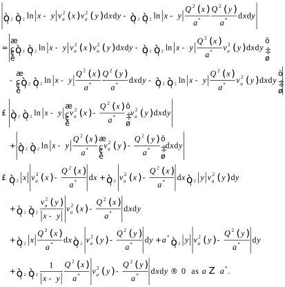
(3.24)

We now give the lower estimate of e( a ) as a↗ a * . It follows from (1.11), (3.5) and (3.24) that

e( a )=E( u a ) = 1 2 ε a −2 ( ∫ ℝ 2 | ∇ v a | 2 dx − a * 2 ∫ ℝ 2 K ( ε a x+ x a ) v a 4 dx )+ 1 2 ∫ ℝ 2 | ε a x+ x a | 2 v a 2 ( x )dx    + 1 4 ln ε a + 1 4 ∫ ℝ 2 ∫ ℝ 2 ln | x−y | v a 2 ( x ) v a 2 ( y )dxdy    + 1 4 ( a * −a ) ε a −2 ∫ ℝ 2 K ( ε a x+ x a ) v a 4 dx ≥ 1 4 ( a * −a ) ε a −2 ∫ ℝ 2 v a 4 dx + 1 4 ln ε a + 1 4 ∫ ℝ 2 ∫ ℝ 2 ln | x−y | v a 2 ( x ) v a 2 ( y )dxdy = a * −a 2 a * ( 1+o( 1 ) ) ε a −2 + 1 4 ln ε a    + 1 4 ( a * ) 2 ( 1+o( 1 ) ) ∫ ℝ 2 ∫ ℝ 2 ln | x−y | Q 2 ( x ) Q 2 ( y )dxdy ≥ 1 8 + 1 8 ln4( a * −a )− 1 8 ln a *    + 1 4 ( a * ) 2 ∫ ℝ 2 ∫ ℝ 2 ln | x−y | Q 2 ( x ) Q 2 ( y )dxdy+o( 1 )   as  a↗ a * , (3.25)

where the identity in the above inequality is achieved at ε a >0 satisfying (3.22), i.e., ε a =2 a * −a a * ( 1+o( 1 ) ) as a↗ a * . We now conclude from (3.23) and (3.25) that

e( a )≈ 1 8 + 1 8 ln4( a * −a )− 1 8 ln a *           + 1 4 ( a * ) 2 ∫ ℝ 2 ∫ ℝ 2 ln | x−y | Q 2 ( x ) Q 2 ( y )dxdy   as  a↗ a * ,

and ε a >0 satisfies (3.22). Moreover, because v a → Q a * in X as a↗ a * , we obtain from Lemma 3.1 that

lim a↗ a * 2 a * −a a * u a ( 2 a * −a a * x+ x a )= Q( x ) a *    in  X.

This completes the proof of Theorem 1.2.

Through relevant proofs and discussions, the existence of minimizers for e( a ) and the refined limiting behavior of positive minimizers for e( a ) have been analyzed as a↗ a * . These mathematical conclusions provide a theoretical basis for the stability of complex quantum systems and physical phenomena under extreme conditions. In future research, we can discuss the local uniqueness of constraint minimizers as a↗ a * to refine the results.

Conflicts of Interest

The authors declare no conflicts of interest.

Conflicts of Interest

The authors declare no conflicts of interest.

References

[1] Benci, V. and Fortunato, D. (1998) An Eigenvalue Problem for the Schrödinger-Maxwell Equations. Topological Methods in Nonlinear Analysis, 11, 283-293.[CrossRef]
[2] D’Aprile, T. and Mugnai, D. (2004) Solitary Waves for Nonlinear Klein-Gordon-Maxwell and Schrödinger-Maxwell Equations. Proceedings of the Royal Society of Edinburgh: Section A Mathematics, 134, 893-906.[CrossRef]
[3] Ruiz, D. (2005) Semiclassical States for Coupled Schrödinger-Maxwell Equations: Concentration around a Sphere. Mathematical Models and Methods in Applied Sciences, 15, 141-164.[CrossRef]
[4] Arnold, A. (1996) Self-Consistent Relaxation-Time Models in Quantum Mechanics. Communications in Partial Differential Equations, 21, 473-506.[CrossRef]
[5] Benci, V. and Fortunato, D.F. (2002) Solitary Waves of the Nonlinear Klein-Gordon Equation Coupled with the Maxwell Equations. Reviews in Mathematical Physics, 14, 409-420.[CrossRef]
[6] Bokanowski, O., López, J.L. and Soler, J. (2003) On an Exchange Interaction Model for Quantum Transport: The Schrödinger-Poisson-Slater System. Mathematical Models and Methods in Applied Sciences, 13, 1397-1412.[CrossRef]
[7] Garnier, J., Baudin, K., Fusaro, A. and Picozzi, A. (2021) Incoherent Localized Structures and Hidden Coherent Solitons from the Gravitational Instability of the Schrödinger-Poisson Equation. Physical Review E, 104, Article ID: 054205.[CrossRef] [PubMed]
[8] Benguria, R., Brezis, H. and Lieb, E.H. (1981) The Thomas-Fermi-Von Weizsäcker Theory of Atoms and Molecules. Communications in Mathematical Physics, 79, 167-180.[CrossRef]
[9] Lions, P.L. (1987) Solutions of Hartree-Fock Equations for Coulomb Systems. Communications in Mathematical Physics, 109, 33-97.[CrossRef]
[10] Catto, I., Dolbeault, J., Sánchez, O. and Soler, J. (2013) Existence of Steady States for the Maxwell-Schrödinger-Poisson System: Exploring the Applicability of the Concentration-Compactness Principle. Mathematical Models and Methods in Applied Sciences, 23, 1915-1938.[CrossRef]
[11] Sánchez, Ó. and Soler, J. (2004) Long-Time Dynamics of the Schrödinger-Poisson-Slater System. Journal of Statistical Physics, 114, 179-204.[CrossRef]
[12] Bartsch, T., Qi, S. and Zou, W. (2024) Normalized Solutions to Schrödinger Equations with Potential and Inhomogeneous Nonlinearities on Large Smooth Domains. Mathematische Annalen, 390, 4813-4859.[CrossRef]
[13] Deng, Y., Guo, Y. and Lu, L. (2014) On the Collapse and Concentration of Bose-Einstein Condensates with Inhomogeneous Attractive Interactions. Calculus of Variations and Partial Differential Equations, 54, 99-118.[CrossRef]
[14] Deng, Y., Guo, Y. and Lu, L. (2018) Threshold Behavior and Uniqueness of Ground States for Mass Critical Inhomogeneous Schrödinger Equations. Journal of Mathematical Physics, 59, Article ID: 011503.[CrossRef]
[15] Shu, M. and Wen, L. (2024) Normalized Solutions for Planar Schrödinger-Poisson System with a Positive Potential. Discrete and Continuous Dynamical Systems—S, 17, 3420-3435.[CrossRef]
[16] Guo, Y., Liang, W. and Li, Y. (2023) Existence and Uniqueness of Constraint Minimizers for the Planar Schrödinger-Poisson System with Logarithmic Potentials. Journal of Differential Equations, 369, 299-352.[CrossRef]
[17] Wang, C. and Zhang, S. (2025) Uniqueness of Minimizers for the Mass Subcritical Planar Schrödinger-Poisson System with Logarithmic Convolution Potential. Discrete and Continuous Dynamical Systems, 45, 794-820.[CrossRef]
[18] Xu, Y. and Luo, H. (2024) Normalized Solutions for Nonautonomous Schrödinger-Poisson Equations. Zeitschrift für angewandte Mathematik und Physik, 75, Article No. 86.[CrossRef]
[19] Zhang, J. (2000) Stability of Standing Waves for Nonlinear Schrödinger Equations with Unbounded Potentials. Zeitschrift für angewandte Mathematik und Physik, 51, 498-503.[CrossRef]
[20] Cingolani, S. and Weth, T. (2016) On the Planar Schrödinger-Poisson System. Annales de l’Institut Henri Poincaré C, Analyse non linéaire, 33, 169-197.[CrossRef]
[21] Lieb, E.H. and Loss, M. (2001) Analysis, Second Edition.
[22] Guo, Y., Luo, Y. and Peng, S. (2021) Local Uniqueness of Ground States for Rotating Bose-Einstein Condensates with Attractive Interactions. Calculus of Variations and Partial Differential Equations, 60, Article No. 237.[CrossRef]
[23] Gidas, B., Ni, W.M. and Nirenberg, L. (1981) Symmetry of Positive Solutions of Nonlinear Elliptic Equations in . Mathematical Analysis and Applications Part A. Advances in Mathematics Supplementary Studies, 7, 369-402.
[24] Weinstein, M.I. (1983) Nonlinear Schrödinger Equations and Sharp Interpolation Estimates. Communications in Mathematical Physics, 87, 567-576.[CrossRef]
[25] Han, Q. and Lin, F.H. (2011) Elliptic Partial Differential Equations. Courant Lecture Notes in Mathematics, 1.
[26] Willem, M. and Theorems, M. (1996) Progress in Nonlinear Differential Equations and Their Applications. Birkhäuser Boston, Inc.

Copyright © 2026 by authors and Scientific Research Publishing Inc.

Creative Commons License

This work and the related PDF file are licensed under a Creative Commons Attribution 4.0 International License.