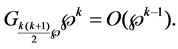
<?xml version="1.0" encoding="UTF-8"?><!DOCTYPE article  PUBLIC "-//NLM//DTD Journal Publishing DTD v3.0 20080202//EN" "http://dtd.nlm.nih.gov/publishing/3.0/journalpublishing3.dtd"><article xmlns:mml="http://www.w3.org/1998/Math/MathML" xmlns:xlink="http://www.w3.org/1999/xlink" dtd-version="3.0" xml:lang="en" article-type="research article"><front><journal-meta><journal-id journal-id-type="publisher-id">JAMP</journal-id><journal-title-group><journal-title>Journal of Applied Mathematics and Physics</journal-title></journal-title-group><issn pub-type="epub">2327-4352</issn><publisher><publisher-name>Scientific Research Publishing</publisher-name></publisher></journal-meta><article-meta><article-id pub-id-type="doi">10.4236/jamp.2016.44093</article-id><article-id pub-id-type="publisher-id">JAMP-66587</article-id><article-categories><subj-group subj-group-type="heading"><subject>Articles</subject></subj-group><subj-group subj-group-type="Discipline-v2"><subject>Physics&amp;Mathematics</subject></subj-group></article-categories><title-group><article-title>
 
 
  Weierstrass’ Elliptic Function Solutions to the Autonomous Limit of the String Equation
 
</article-title></title-group><contrib-group><contrib contrib-type="author" xlink:type="simple"><name name-style="western"><surname>Yoshikatsu</surname><given-names>Sasaki</given-names></name><xref ref-type="aff" rid="aff1"><sub>1</sub></xref></contrib></contrib-group><aff id="aff1"><label>1</label><addr-line>Department of Mathematics, Hiroshima University, Higashi-Hiroshima, Japan</addr-line></aff><author-notes><corresp id="cor1">* E-mail:</corresp></author-notes><pub-date pub-type="epub"><day>13</day><month>04</month><year>2016</year></pub-date><volume>04</volume><issue>04</issue><fpage>857</fpage><lpage>862</lpage><history><date date-type="received"><day>4</day>	<month>January</month>	<year>2016</year></date><date date-type="rev-recd"><day>accepted</day>	<month>23</month>	<year>April</year>	</date><date date-type="accepted"><day>30</day>	<month>April</month>	<year>2016</year></date></history><permissions><copyright-statement>&#169; Copyright  2014 by authors and Scientific Research Publishing Inc. </copyright-statement><copyright-year>2014</copyright-year><license><license-p>This work is licensed under the Creative Commons Attribution International License (CC BY). http://creativecommons.org/licenses/by/4.0/</license-p></license></permissions><abstract><p>
 
 
   In this article, we study the string equation of type (2, 2n + 1), which is derived from 2D gravity theory or the string theory. We consider the equation as a 2n-th order analogue of the first Painlev&#233;equation, take the autonomous limit, and solve it concretely by use of the Weierstrass’ elliptic function. 
 
</p></abstract><kwd-group><kwd>Painlev&#233; Hierarchy</kwd><kwd> String Equation</kwd><kwd> Elliptic Function</kwd></kwd-group></article-meta></front><body><sec id="s1"><title>1. Introduction</title><p>1.1. The String Equation of Type (2, 2n + 1)</p><p>Let <inline-formula><inline-graphic xlink:href="http://html.scirp.org/file/66587x4.png" xlink:type="simple"/></inline-formula> stand for the differentiation w.r.t.<inline-formula><inline-graphic xlink:href="http://html.scirp.org/file/66587x5.png" xlink:type="simple"/></inline-formula>, and <inline-formula><inline-graphic xlink:href="http://html.scirp.org/file/66587x6.png" xlink:type="simple"/></inline-formula> stand for the inverse operator of<inline-formula><inline-graphic xlink:href="http://html.scirp.org/file/66587x7.png" xlink:type="simple"/></inline-formula>. Consider the commutator equation of ordinary differential operators</p><disp-formula id="scirp.66587-formula355"><label>(1)</label><graphic position="anchor" xlink:href="http://html.scirp.org/file/66587x8.png"  xlink:type="simple"/></disp-formula><p>for a couple of positive integers<inline-formula><inline-graphic xlink:href="http://html.scirp.org/file/66587x9.png" xlink:type="simple"/></inline-formula>. The above equation is called the string Equation (or Douglas equation) of type<inline-formula><inline-graphic xlink:href="http://html.scirp.org/file/66587x10.png" xlink:type="simple"/></inline-formula>, and appears in the string theory or the theory of 2D quantum gravity [<xref ref-type="bibr" rid="scirp.66587-ref1">1</xref>]-[<xref ref-type="bibr" rid="scirp.66587-ref8">8</xref>]. In the followings, we set <inline-formula><inline-graphic xlink:href="http://html.scirp.org/file/66587x11.png" xlink:type="simple"/></inline-formula> for a positive integer<inline-formula><inline-graphic xlink:href="http://html.scirp.org/file/66587x12.png" xlink:type="simple"/></inline-formula>.</p><p>In the case where<inline-formula><inline-graphic xlink:href="http://html.scirp.org/file/66587x13.png" xlink:type="simple"/></inline-formula>, the string equation is written as an ODE satisfied by the potential <inline-formula><inline-graphic xlink:href="http://html.scirp.org/file/66587x14.png" xlink:type="simple"/></inline-formula> of Sturm-Liouville operator<inline-formula><inline-graphic xlink:href="http://html.scirp.org/file/66587x15.png" xlink:type="simple"/></inline-formula>, and then, by a fractional linear transformation, it is reduced to the first Painlev&#233; equation [<xref ref-type="bibr" rid="scirp.66587-ref9">9</xref>]-[<xref ref-type="bibr" rid="scirp.66587-ref11">11</xref>]. In fact, the string equation of type <inline-formula><inline-graphic xlink:href="http://html.scirp.org/file/66587x16.png" xlink:type="simple"/></inline-formula></p><disp-formula id="scirp.66587-formula356"><label>(2)</label><graphic position="anchor" xlink:href="http://html.scirp.org/file/66587x17.png"  xlink:type="simple"/></disp-formula><p>i.e.</p><disp-formula id="scirp.66587-formula357"><label>(3)</label><graphic position="anchor" xlink:href="http://html.scirp.org/file/66587x18.png"  xlink:type="simple"/></disp-formula><p>is written as an equation <inline-formula><inline-graphic xlink:href="http://html.scirp.org/file/66587x19.png" xlink:type="simple"/></inline-formula> or integrated one <inline-formula><inline-graphic xlink:href="http://html.scirp.org/file/66587x20.png" xlink:type="simple"/></inline-formula> with integral constants <inline-formula><inline-graphic xlink:href="http://html.scirp.org/file/66587x20.png" xlink:type="simple"/></inline-formula><inline-formula><inline-graphic xlink:href="http://html.scirp.org/file/66587x21.png" xlink:type="simple"/></inline-formula> and <inline-formula><inline-graphic xlink:href="http://html.scirp.org/file/66587x20.png" xlink:type="simple"/></inline-formula><inline-formula><inline-graphic xlink:href="http://html.scirp.org/file/66587x21.png" xlink:type="simple"/></inline-formula><inline-formula><inline-graphic xlink:href="http://html.scirp.org/file/66587x22.png" xlink:type="simple"/></inline-formula> by putting <inline-formula><inline-graphic xlink:href="http://html.scirp.org/file/66587x20.png" xlink:type="simple"/></inline-formula><inline-formula><inline-graphic xlink:href="http://html.scirp.org/file/66587x21.png" xlink:type="simple"/></inline-formula><inline-formula><inline-graphic xlink:href="http://html.scirp.org/file/66587x22.png" xlink:type="simple"/></inline-formula><inline-formula><inline-graphic xlink:href="http://html.scirp.org/file/66587x23.png" xlink:type="simple"/></inline-formula> which is reduced to the first Painlev&#233; equation</p><disp-formula id="scirp.66587-formula358"><label>(4)</label><graphic position="anchor" xlink:href="http://html.scirp.org/file/66587x24.png"  xlink:type="simple"/></disp-formula><p>by replacement<inline-formula><inline-graphic xlink:href="http://html.scirp.org/file/66587x25.png" xlink:type="simple"/></inline-formula>, <inline-formula><inline-graphic xlink:href="http://html.scirp.org/file/66587x25.png" xlink:type="simple"/></inline-formula><inline-formula><inline-graphic xlink:href="http://html.scirp.org/file/66587x27.png" xlink:type="simple"/></inline-formula><inline-formula><inline-graphic xlink:href="http://html.scirp.org/file/66587x25.png" xlink:type="simple"/></inline-formula><inline-formula><inline-graphic xlink:href="http://html.scirp.org/file/66587x27.png" xlink:type="simple"/></inline-formula><inline-formula><inline-graphic xlink:href="http://html.scirp.org/file/66587x26.png" xlink:type="simple"/></inline-formula>with<inline-formula><inline-graphic xlink:href="http://html.scirp.org/file/66587x25.png" xlink:type="simple"/></inline-formula><inline-formula><inline-graphic xlink:href="http://html.scirp.org/file/66587x27.png" xlink:type="simple"/></inline-formula><inline-formula><inline-graphic xlink:href="http://html.scirp.org/file/66587x26.png" xlink:type="simple"/></inline-formula><inline-formula><inline-graphic xlink:href="http://html.scirp.org/file/66587x28.png" xlink:type="simple"/></inline-formula>, <inline-formula><inline-graphic xlink:href="http://html.scirp.org/file/66587x25.png" xlink:type="simple"/></inline-formula><inline-formula><inline-graphic xlink:href="http://html.scirp.org/file/66587x27.png" xlink:type="simple"/></inline-formula><inline-formula><inline-graphic xlink:href="http://html.scirp.org/file/66587x26.png" xlink:type="simple"/></inline-formula><inline-formula><inline-graphic xlink:href="http://html.scirp.org/file/66587x28.png" xlink:type="simple"/></inline-formula><inline-formula><inline-graphic xlink:href="http://html.scirp.org/file/66587x29.png" xlink:type="simple"/></inline-formula>, <inline-formula><inline-graphic xlink:href="http://html.scirp.org/file/66587x25.png" xlink:type="simple"/></inline-formula><inline-formula><inline-graphic xlink:href="http://html.scirp.org/file/66587x27.png" xlink:type="simple"/></inline-formula><inline-formula><inline-graphic xlink:href="http://html.scirp.org/file/66587x26.png" xlink:type="simple"/></inline-formula><inline-formula><inline-graphic xlink:href="http://html.scirp.org/file/66587x28.png" xlink:type="simple"/></inline-formula><inline-formula><inline-graphic xlink:href="http://html.scirp.org/file/66587x29.png" xlink:type="simple"/></inline-formula><inline-formula><inline-graphic xlink:href="http://html.scirp.org/file/66587x30.png" xlink:type="simple"/></inline-formula>,<inline-formula><inline-graphic xlink:href="http://html.scirp.org/file/66587x25.png" xlink:type="simple"/></inline-formula><inline-formula><inline-graphic xlink:href="http://html.scirp.org/file/66587x27.png" xlink:type="simple"/></inline-formula><inline-formula><inline-graphic xlink:href="http://html.scirp.org/file/66587x26.png" xlink:type="simple"/></inline-formula><inline-formula><inline-graphic xlink:href="http://html.scirp.org/file/66587x28.png" xlink:type="simple"/></inline-formula><inline-formula><inline-graphic xlink:href="http://html.scirp.org/file/66587x29.png" xlink:type="simple"/></inline-formula><inline-formula><inline-graphic xlink:href="http://html.scirp.org/file/66587x30.png" xlink:type="simple"/></inline-formula><inline-formula><inline-graphic xlink:href="http://html.scirp.org/file/66587x31.png" xlink:type="simple"/></inline-formula>.</p><p>In the case where<inline-formula><inline-graphic xlink:href="http://html.scirp.org/file/66587x32.png" xlink:type="simple"/></inline-formula>, the string equation</p><disp-formula id="scirp.66587-formula359"><label>(5)</label><graphic position="anchor" xlink:href="http://html.scirp.org/file/66587x33.png"  xlink:type="simple"/></disp-formula><p>is similarly reduced to</p><disp-formula id="scirp.66587-formula360"><graphic  xlink:href="http://html.scirp.org/file/66587x34.png"  xlink:type="simple"/></disp-formula><p>by replacement<inline-formula><inline-graphic xlink:href="http://html.scirp.org/file/66587x35.png" xlink:type="simple"/></inline-formula>, <inline-formula><inline-graphic xlink:href="http://html.scirp.org/file/66587x35.png" xlink:type="simple"/></inline-formula><inline-formula><inline-graphic xlink:href="http://html.scirp.org/file/66587x37.png" xlink:type="simple"/></inline-formula><inline-formula><inline-graphic xlink:href="http://html.scirp.org/file/66587x35.png" xlink:type="simple"/></inline-formula><inline-formula><inline-graphic xlink:href="http://html.scirp.org/file/66587x37.png" xlink:type="simple"/></inline-formula><inline-formula><inline-graphic xlink:href="http://html.scirp.org/file/66587x36.png" xlink:type="simple"/></inline-formula>with<inline-formula><inline-graphic xlink:href="http://html.scirp.org/file/66587x35.png" xlink:type="simple"/></inline-formula><inline-formula><inline-graphic xlink:href="http://html.scirp.org/file/66587x37.png" xlink:type="simple"/></inline-formula><inline-formula><inline-graphic xlink:href="http://html.scirp.org/file/66587x36.png" xlink:type="simple"/></inline-formula><inline-formula><inline-graphic xlink:href="http://html.scirp.org/file/66587x38.png" xlink:type="simple"/></inline-formula>, <inline-formula><inline-graphic xlink:href="http://html.scirp.org/file/66587x35.png" xlink:type="simple"/></inline-formula><inline-formula><inline-graphic xlink:href="http://html.scirp.org/file/66587x37.png" xlink:type="simple"/></inline-formula><inline-formula><inline-graphic xlink:href="http://html.scirp.org/file/66587x36.png" xlink:type="simple"/></inline-formula><inline-formula><inline-graphic xlink:href="http://html.scirp.org/file/66587x38.png" xlink:type="simple"/></inline-formula><inline-formula><inline-graphic xlink:href="http://html.scirp.org/file/66587x39.png" xlink:type="simple"/></inline-formula>and suitable<inline-formula><inline-graphic xlink:href="http://html.scirp.org/file/66587x35.png" xlink:type="simple"/></inline-formula><inline-formula><inline-graphic xlink:href="http://html.scirp.org/file/66587x37.png" xlink:type="simple"/></inline-formula><inline-formula><inline-graphic xlink:href="http://html.scirp.org/file/66587x36.png" xlink:type="simple"/></inline-formula><inline-formula><inline-graphic xlink:href="http://html.scirp.org/file/66587x38.png" xlink:type="simple"/></inline-formula><inline-formula><inline-graphic xlink:href="http://html.scirp.org/file/66587x39.png" xlink:type="simple"/></inline-formula><inline-formula><inline-graphic xlink:href="http://html.scirp.org/file/66587x40.png" xlink:type="simple"/></inline-formula>. That is the 4th order equation of the first Painlev&#233; hierarchy.</p><sec id="s1_1"><title>1.2. The First Painlev&#233; Hierarchy</title><p>Now we recall the definition of the first Painlev&#233; hierarchy. Consider the serial equations</p><disp-formula id="scirp.66587-formula361"><label>(6)</label><graphic position="anchor" xlink:href="http://html.scirp.org/file/66587x41.png"  xlink:type="simple"/></disp-formula><p>for<inline-formula><inline-graphic xlink:href="http://html.scirp.org/file/66587x42.png" xlink:type="simple"/></inline-formula>, where <inline-formula><inline-graphic xlink:href="http://html.scirp.org/file/66587x42.png" xlink:type="simple"/></inline-formula><inline-formula><inline-graphic xlink:href="http://html.scirp.org/file/66587x43.png" xlink:type="simple"/></inline-formula> is an expression of a given meromorphic function <inline-formula><inline-graphic xlink:href="http://html.scirp.org/file/66587x42.png" xlink:type="simple"/></inline-formula><inline-formula><inline-graphic xlink:href="http://html.scirp.org/file/66587x43.png" xlink:type="simple"/></inline-formula><inline-formula><inline-graphic xlink:href="http://html.scirp.org/file/66587x44.png" xlink:type="simple"/></inline-formula> defined by <inline-formula><inline-graphic xlink:href="http://html.scirp.org/file/66587x42.png" xlink:type="simple"/></inline-formula><inline-formula><inline-graphic xlink:href="http://html.scirp.org/file/66587x43.png" xlink:type="simple"/></inline-formula><inline-formula><inline-graphic xlink:href="http://html.scirp.org/file/66587x44.png" xlink:type="simple"/></inline-formula><inline-formula><inline-graphic xlink:href="http://html.scirp.org/file/66587x45.png" xlink:type="simple"/></inline-formula> and <inline-formula><inline-graphic xlink:href="http://html.scirp.org/file/66587x42.png" xlink:type="simple"/></inline-formula><inline-formula><inline-graphic xlink:href="http://html.scirp.org/file/66587x43.png" xlink:type="simple"/></inline-formula><inline-formula><inline-graphic xlink:href="http://html.scirp.org/file/66587x44.png" xlink:type="simple"/></inline-formula><inline-formula><inline-graphic xlink:href="http://html.scirp.org/file/66587x45.png" xlink:type="simple"/></inline-formula><inline-formula><inline-graphic xlink:href="http://html.scirp.org/file/66587x46.png" xlink:type="simple"/></inline-formula> with<inline-formula><inline-graphic xlink:href="http://html.scirp.org/file/66587x42.png" xlink:type="simple"/></inline-formula><inline-formula><inline-graphic xlink:href="http://html.scirp.org/file/66587x43.png" xlink:type="simple"/></inline-formula><inline-formula><inline-graphic xlink:href="http://html.scirp.org/file/66587x44.png" xlink:type="simple"/></inline-formula><inline-formula><inline-graphic xlink:href="http://html.scirp.org/file/66587x45.png" xlink:type="simple"/></inline-formula><inline-formula><inline-graphic xlink:href="http://html.scirp.org/file/66587x46.png" xlink:type="simple"/></inline-formula><inline-formula><inline-graphic xlink:href="http://html.scirp.org/file/66587x47.png" xlink:type="simple"/></inline-formula>. The equations are derived from the singular manifold equation for the KdV hierarchy, and we call them the first Painlev&#233; hierarchy [<xref ref-type="bibr" rid="scirp.66587-ref10">10</xref>] [<xref ref-type="bibr" rid="scirp.66587-ref12">12</xref>] [<xref ref-type="bibr" rid="scirp.66587-ref13">13</xref>]. For example, <inline-formula><inline-graphic xlink:href="http://html.scirp.org/file/66587x42.png" xlink:type="simple"/></inline-formula><inline-formula><inline-graphic xlink:href="http://html.scirp.org/file/66587x43.png" xlink:type="simple"/></inline-formula><inline-formula><inline-graphic xlink:href="http://html.scirp.org/file/66587x44.png" xlink:type="simple"/></inline-formula><inline-formula><inline-graphic xlink:href="http://html.scirp.org/file/66587x45.png" xlink:type="simple"/></inline-formula><inline-formula><inline-graphic xlink:href="http://html.scirp.org/file/66587x46.png" xlink:type="simple"/></inline-formula><inline-formula><inline-graphic xlink:href="http://html.scirp.org/file/66587x47.png" xlink:type="simple"/></inline-formula><inline-formula><inline-graphic xlink:href="http://html.scirp.org/file/66587x48.png" xlink:type="simple"/></inline-formula>, where <inline-formula><inline-graphic xlink:href="http://html.scirp.org/file/66587x42.png" xlink:type="simple"/></inline-formula><inline-formula><inline-graphic xlink:href="http://html.scirp.org/file/66587x43.png" xlink:type="simple"/></inline-formula><inline-formula><inline-graphic xlink:href="http://html.scirp.org/file/66587x44.png" xlink:type="simple"/></inline-formula><inline-formula><inline-graphic xlink:href="http://html.scirp.org/file/66587x45.png" xlink:type="simple"/></inline-formula><inline-formula><inline-graphic xlink:href="http://html.scirp.org/file/66587x46.png" xlink:type="simple"/></inline-formula><inline-formula><inline-graphic xlink:href="http://html.scirp.org/file/66587x47.png" xlink:type="simple"/></inline-formula><inline-formula><inline-graphic xlink:href="http://html.scirp.org/file/66587x48.png" xlink:type="simple"/></inline-formula><inline-formula><inline-graphic xlink:href="http://html.scirp.org/file/66587x49.png" xlink:type="simple"/></inline-formula> is an integral constant. In the followings, each <inline-formula><inline-graphic xlink:href="http://html.scirp.org/file/66587x42.png" xlink:type="simple"/></inline-formula><inline-formula><inline-graphic xlink:href="http://html.scirp.org/file/66587x43.png" xlink:type="simple"/></inline-formula><inline-formula><inline-graphic xlink:href="http://html.scirp.org/file/66587x44.png" xlink:type="simple"/></inline-formula><inline-formula><inline-graphic xlink:href="http://html.scirp.org/file/66587x45.png" xlink:type="simple"/></inline-formula><inline-formula><inline-graphic xlink:href="http://html.scirp.org/file/66587x46.png" xlink:type="simple"/></inline-formula><inline-formula><inline-graphic xlink:href="http://html.scirp.org/file/66587x47.png" xlink:type="simple"/></inline-formula><inline-formula><inline-graphic xlink:href="http://html.scirp.org/file/66587x48.png" xlink:type="simple"/></inline-formula><inline-formula><inline-graphic xlink:href="http://html.scirp.org/file/66587x49.png" xlink:type="simple"/></inline-formula><inline-formula><inline-graphic xlink:href="http://html.scirp.org/file/66587x50.png" xlink:type="simple"/></inline-formula> is also an integral constant.</p><p>If<inline-formula><inline-graphic xlink:href="http://html.scirp.org/file/66587x51.png" xlink:type="simple"/></inline-formula>, we have <inline-formula><inline-graphic xlink:href="http://html.scirp.org/file/66587x51.png" xlink:type="simple"/></inline-formula><inline-formula><inline-graphic xlink:href="http://html.scirp.org/file/66587x52.png" xlink:type="simple"/></inline-formula> then <inline-formula><inline-graphic xlink:href="http://html.scirp.org/file/66587x51.png" xlink:type="simple"/></inline-formula><inline-formula><inline-graphic xlink:href="http://html.scirp.org/file/66587x52.png" xlink:type="simple"/></inline-formula><inline-formula><inline-graphic xlink:href="http://html.scirp.org/file/66587x53.png" xlink:type="simple"/></inline-formula> essentially coinsides with the first Painlev&#233; equation.</p><p>If<inline-formula><inline-graphic xlink:href="http://html.scirp.org/file/66587x54.png" xlink:type="simple"/></inline-formula>, we have <inline-formula><inline-graphic xlink:href="http://html.scirp.org/file/66587x54.png" xlink:type="simple"/></inline-formula><inline-formula><inline-graphic xlink:href="http://html.scirp.org/file/66587x55.png" xlink:type="simple"/></inline-formula> and then</p><disp-formula id="scirp.66587-formula362"><label>(7)</label><graphic position="anchor" xlink:href="http://html.scirp.org/file/66587x56.png"  xlink:type="simple"/></disp-formula><p>Again, it essentially coinsides with (5), i.e. the 4th order equation of the first Painlev&#233; hierarchy.</p><p>As proved by K. Takasaki [<xref ref-type="bibr" rid="scirp.66587-ref8">8</xref>], the string equation of type <inline-formula><inline-graphic xlink:href="http://html.scirp.org/file/66587x57.png" xlink:type="simple"/></inline-formula> is equivalent to (6). So, in this article, we also call (6) the string equation of type<inline-formula><inline-graphic xlink:href="http://html.scirp.org/file/66587x57.png" xlink:type="simple"/></inline-formula><inline-formula><inline-graphic xlink:href="http://html.scirp.org/file/66587x58.png" xlink:type="simple"/></inline-formula>.</p><p>Note that S. Shimomura [<xref ref-type="bibr" rid="scirp.66587-ref14">14</xref>] proved the theorems as follows.</p><p>Theorem A [<xref ref-type="bibr" rid="scirp.66587-ref14">14</xref>]. Each <inline-formula><inline-graphic xlink:href="http://html.scirp.org/file/66587x59.png" xlink:type="simple"/></inline-formula> is a differential polynomial of 2n-th order, i.e. each (6) is an ordinary differential equation of 2n-th order.</p><p>Theorem B [<xref ref-type="bibr" rid="scirp.66587-ref14">14</xref>]. At each pole<inline-formula><inline-graphic xlink:href="http://html.scirp.org/file/66587x60.png" xlink:type="simple"/></inline-formula>, the meromorphic solution to (6) has the form</p><disp-formula id="scirp.66587-formula363"><graphic  xlink:href="http://html.scirp.org/file/66587x61.png"  xlink:type="simple"/></disp-formula><p>for some positive integer<inline-formula><inline-graphic xlink:href="http://html.scirp.org/file/66587x62.png" xlink:type="simple"/></inline-formula>.</p><p>The author proved a theorem similar to Theorem A for the second Painlev&#233; hierarchy [<xref ref-type="bibr" rid="scirp.66587-ref15">15</xref>], and, in its proof, auxiliary differential polynomials play important roles. So, for the first Painlev&#233; hierarchy as well, the auxiliary differential polynomials should exist. Recall them.</p><p>Theorem C [<xref ref-type="bibr" rid="scirp.66587-ref16">16</xref>]. Define <inline-formula><inline-graphic xlink:href="http://html.scirp.org/file/66587x63.png" xlink:type="simple"/></inline-formula> by<inline-formula><inline-graphic xlink:href="http://html.scirp.org/file/66587x63.png" xlink:type="simple"/></inline-formula><inline-formula><inline-graphic xlink:href="http://html.scirp.org/file/66587x64.png" xlink:type="simple"/></inline-formula>. Then each <inline-formula><inline-graphic xlink:href="http://html.scirp.org/file/66587x63.png" xlink:type="simple"/></inline-formula><inline-formula><inline-graphic xlink:href="http://html.scirp.org/file/66587x64.png" xlink:type="simple"/></inline-formula><inline-formula><inline-graphic xlink:href="http://html.scirp.org/file/66587x65.png" xlink:type="simple"/></inline-formula> is a differential polynomial of 2n-th order.</p></sec><sec id="s1_2"><title>1.3. Autonomous Limits</title><p>The first Painlev&#233; equation has the autonomous limit [<xref ref-type="bibr" rid="scirp.66587-ref9">9</xref>]. Replacing <inline-formula><inline-graphic xlink:href="http://html.scirp.org/file/66587x66.png" xlink:type="simple"/></inline-formula> by <inline-formula><inline-graphic xlink:href="http://html.scirp.org/file/66587x66.png" xlink:type="simple"/></inline-formula><inline-formula><inline-graphic xlink:href="http://html.scirp.org/file/66587x67.png" xlink:type="simple"/></inline-formula> with a constant<inline-formula><inline-graphic xlink:href="http://html.scirp.org/file/66587x66.png" xlink:type="simple"/></inline-formula><inline-formula><inline-graphic xlink:href="http://html.scirp.org/file/66587x67.png" xlink:type="simple"/></inline-formula><inline-formula><inline-graphic xlink:href="http://html.scirp.org/file/66587x68.png" xlink:type="simple"/></inline-formula>, and taking limit<inline-formula><inline-graphic xlink:href="http://html.scirp.org/file/66587x66.png" xlink:type="simple"/></inline-formula><inline-formula><inline-graphic xlink:href="http://html.scirp.org/file/66587x67.png" xlink:type="simple"/></inline-formula><inline-formula><inline-graphic xlink:href="http://html.scirp.org/file/66587x68.png" xlink:type="simple"/></inline-formula><inline-formula><inline-graphic xlink:href="http://html.scirp.org/file/66587x69.png" xlink:type="simple"/></inline-formula>, we obtain <inline-formula><inline-graphic xlink:href="http://html.scirp.org/file/66587x66.png" xlink:type="simple"/></inline-formula><inline-formula><inline-graphic xlink:href="http://html.scirp.org/file/66587x67.png" xlink:type="simple"/></inline-formula><inline-formula><inline-graphic xlink:href="http://html.scirp.org/file/66587x68.png" xlink:type="simple"/></inline-formula><inline-formula><inline-graphic xlink:href="http://html.scirp.org/file/66587x69.png" xlink:type="simple"/></inline-formula><inline-formula><inline-graphic xlink:href="http://html.scirp.org/file/66587x70.png" xlink:type="simple"/></inline-formula> which is satisfied by the Weierstrass’ elliptic function, i.e.</p><disp-formula id="scirp.66587-formula364"><graphic  xlink:href="http://html.scirp.org/file/66587x71.png"  xlink:type="simple"/></disp-formula><p>where <inline-formula><inline-graphic xlink:href="http://html.scirp.org/file/66587x72.png" xlink:type="simple"/></inline-formula> for some <inline-formula><inline-graphic xlink:href="http://html.scirp.org/file/66587x72.png" xlink:type="simple"/></inline-formula><inline-formula><inline-graphic xlink:href="http://html.scirp.org/file/66587x73.png" xlink:type="simple"/></inline-formula> satisfying<inline-formula><inline-graphic xlink:href="http://html.scirp.org/file/66587x72.png" xlink:type="simple"/></inline-formula><inline-formula><inline-graphic xlink:href="http://html.scirp.org/file/66587x73.png" xlink:type="simple"/></inline-formula><inline-formula><inline-graphic xlink:href="http://html.scirp.org/file/66587x74.png" xlink:type="simple"/></inline-formula>. Here <inline-formula><inline-graphic xlink:href="http://html.scirp.org/file/66587x72.png" xlink:type="simple"/></inline-formula><inline-formula><inline-graphic xlink:href="http://html.scirp.org/file/66587x73.png" xlink:type="simple"/></inline-formula><inline-formula><inline-graphic xlink:href="http://html.scirp.org/file/66587x74.png" xlink:type="simple"/></inline-formula><inline-formula><inline-graphic xlink:href="http://html.scirp.org/file/66587x75.png" xlink:type="simple"/></inline-formula> means the sum for<inline-formula><inline-graphic xlink:href="http://html.scirp.org/file/66587x72.png" xlink:type="simple"/></inline-formula><inline-formula><inline-graphic xlink:href="http://html.scirp.org/file/66587x73.png" xlink:type="simple"/></inline-formula><inline-formula><inline-graphic xlink:href="http://html.scirp.org/file/66587x74.png" xlink:type="simple"/></inline-formula><inline-formula><inline-graphic xlink:href="http://html.scirp.org/file/66587x75.png" xlink:type="simple"/></inline-formula><inline-formula><inline-graphic xlink:href="http://html.scirp.org/file/66587x76.png" xlink:type="simple"/></inline-formula>. It is well-known that <inline-formula><inline-graphic xlink:href="http://html.scirp.org/file/66587x72.png" xlink:type="simple"/></inline-formula><inline-formula><inline-graphic xlink:href="http://html.scirp.org/file/66587x73.png" xlink:type="simple"/></inline-formula><inline-formula><inline-graphic xlink:href="http://html.scirp.org/file/66587x74.png" xlink:type="simple"/></inline-formula><inline-formula><inline-graphic xlink:href="http://html.scirp.org/file/66587x75.png" xlink:type="simple"/></inline-formula><inline-formula><inline-graphic xlink:href="http://html.scirp.org/file/66587x76.png" xlink:type="simple"/></inline-formula><inline-formula><inline-graphic xlink:href="http://html.scirp.org/file/66587x77.png" xlink:type="simple"/></inline-formula> is a doubly periodic meromorphic function with two fundamental periods<inline-formula><inline-graphic xlink:href="http://html.scirp.org/file/66587x72.png" xlink:type="simple"/></inline-formula><inline-formula><inline-graphic xlink:href="http://html.scirp.org/file/66587x73.png" xlink:type="simple"/></inline-formula><inline-formula><inline-graphic xlink:href="http://html.scirp.org/file/66587x74.png" xlink:type="simple"/></inline-formula><inline-formula><inline-graphic xlink:href="http://html.scirp.org/file/66587x75.png" xlink:type="simple"/></inline-formula><inline-formula><inline-graphic xlink:href="http://html.scirp.org/file/66587x76.png" xlink:type="simple"/></inline-formula><inline-formula><inline-graphic xlink:href="http://html.scirp.org/file/66587x77.png" xlink:type="simple"/></inline-formula><inline-formula><inline-graphic xlink:href="http://html.scirp.org/file/66587x78.png" xlink:type="simple"/></inline-formula>. <inline-formula><inline-graphic xlink:href="http://html.scirp.org/file/66587x72.png" xlink:type="simple"/></inline-formula><inline-formula><inline-graphic xlink:href="http://html.scirp.org/file/66587x73.png" xlink:type="simple"/></inline-formula><inline-formula><inline-graphic xlink:href="http://html.scirp.org/file/66587x74.png" xlink:type="simple"/></inline-formula><inline-formula><inline-graphic xlink:href="http://html.scirp.org/file/66587x75.png" xlink:type="simple"/></inline-formula><inline-formula><inline-graphic xlink:href="http://html.scirp.org/file/66587x76.png" xlink:type="simple"/></inline-formula><inline-formula><inline-graphic xlink:href="http://html.scirp.org/file/66587x77.png" xlink:type="simple"/></inline-formula><inline-formula><inline-graphic xlink:href="http://html.scirp.org/file/66587x78.png" xlink:type="simple"/></inline-formula><inline-formula><inline-graphic xlink:href="http://html.scirp.org/file/66587x79.png" xlink:type="simple"/></inline-formula>satisfies the differential equation</p><p><inline-formula><inline-graphic xlink:href="http://html.scirp.org/file/66587x80.png" xlink:type="simple"/></inline-formula>and then</p><p><inline-formula><inline-graphic xlink:href="http://html.scirp.org/file/66587x81.png" xlink:type="simple"/></inline-formula>,</p><p>where</p><disp-formula id="scirp.66587-formula365"><graphic  xlink:href="http://html.scirp.org/file/66587x82.png"  xlink:type="simple"/></disp-formula><p>For<inline-formula><inline-graphic xlink:href="http://html.scirp.org/file/66587x83.png" xlink:type="simple"/></inline-formula>, a similar result is valid, i.e.</p><p>Theorem D [<xref ref-type="bibr" rid="scirp.66587-ref17">17</xref>]. The 4th order equation of the first Painlev&#233; hierarchy with suitable parameters</p><disp-formula id="scirp.66587-formula366"><label>(8)</label><graphic position="anchor" xlink:href="http://html.scirp.org/file/66587x84.png"  xlink:type="simple"/></disp-formula><p>is reduced to the autonomous equation</p><disp-formula id="scirp.66587-formula367"><label>(9)</label><graphic position="anchor" xlink:href="http://html.scirp.org/file/66587x85.png"  xlink:type="simple"/></disp-formula><p>by replacing <inline-formula><inline-graphic xlink:href="http://html.scirp.org/file/66587x86.png" xlink:type="simple"/></inline-formula> by<inline-formula><inline-graphic xlink:href="http://html.scirp.org/file/66587x86.png" xlink:type="simple"/></inline-formula><inline-formula><inline-graphic xlink:href="http://html.scirp.org/file/66587x87.png" xlink:type="simple"/></inline-formula>, and taking the limit<inline-formula><inline-graphic xlink:href="http://html.scirp.org/file/66587x86.png" xlink:type="simple"/></inline-formula><inline-formula><inline-graphic xlink:href="http://html.scirp.org/file/66587x87.png" xlink:type="simple"/></inline-formula><inline-formula><inline-graphic xlink:href="http://html.scirp.org/file/66587x88.png" xlink:type="simple"/></inline-formula>.</p><p>Note that the Equation (8) is obtained as a section of the most degenerated 2D Garnier system [<xref ref-type="bibr" rid="scirp.66587-ref18">18</xref>] (see also [<xref ref-type="bibr" rid="scirp.66587-ref19">19</xref>] [<xref ref-type="bibr" rid="scirp.66587-ref20">20</xref>]). The following theorem is not trivial but natural if we consider Theorem D together with Theorem B.</p><p>Theorem E [<xref ref-type="bibr" rid="scirp.66587-ref17">17</xref>]. For suitable<inline-formula><inline-graphic xlink:href="http://html.scirp.org/file/66587x89.png" xlink:type="simple"/></inline-formula>, the autonomous Equation (9) has a solution concretely described as</p><disp-formula id="scirp.66587-formula368"><graphic  xlink:href="http://html.scirp.org/file/66587x90.png"  xlink:type="simple"/></disp-formula></sec><sec id="s1_3"><title>1.4. Results</title><p>A result similar to Theorem D is valid for<inline-formula><inline-graphic xlink:href="http://html.scirp.org/file/66587x91.png" xlink:type="simple"/></inline-formula>.</p><p>Theorem 1.1. The autonomous limit of the string equation of type <inline-formula><inline-graphic xlink:href="http://html.scirp.org/file/66587x92.png" xlink:type="simple"/></inline-formula> is given by</p><disp-formula id="scirp.66587-formula369"><label>(10)</label><graphic position="anchor" xlink:href="http://html.scirp.org/file/66587x93.png"  xlink:type="simple"/></disp-formula><p>where <inline-formula><inline-graphic xlink:href="http://html.scirp.org/file/66587x94.png" xlink:type="simple"/></inline-formula> is a complex parameter.</p><p>Proof. Note that <inline-formula><inline-graphic xlink:href="http://html.scirp.org/file/66587x95.png" xlink:type="simple"/></inline-formula> has the form</p><disp-formula id="scirp.66587-formula370"><graphic  xlink:href="http://html.scirp.org/file/66587x96.png"  xlink:type="simple"/></disp-formula><p>with the weight [<xref ref-type="bibr" rid="scirp.66587-ref14">14</xref>] <inline-formula><inline-graphic xlink:href="http://html.scirp.org/file/66587x97.png" xlink:type="simple"/></inline-formula>defined by <inline-formula><inline-graphic xlink:href="http://html.scirp.org/file/66587x97.png" xlink:type="simple"/></inline-formula><inline-formula><inline-graphic xlink:href="http://html.scirp.org/file/66587x98.png" xlink:type="simple"/></inline-formula> and<inline-formula><inline-graphic xlink:href="http://html.scirp.org/file/66587x97.png" xlink:type="simple"/></inline-formula><inline-formula><inline-graphic xlink:href="http://html.scirp.org/file/66587x98.png" xlink:type="simple"/></inline-formula><inline-formula><inline-graphic xlink:href="http://html.scirp.org/file/66587x99.png" xlink:type="simple"/></inline-formula>. After replacement</p><p><inline-formula><inline-graphic xlink:href="http://html.scirp.org/file/66587x100.png" xlink:type="simple"/></inline-formula>,</p><p>taking the limit<inline-formula><inline-graphic xlink:href="http://html.scirp.org/file/66587x101.png" xlink:type="simple"/></inline-formula>, we obtain the conclusion. <inline-formula><inline-graphic xlink:href="http://html.scirp.org/file/66587x101.png" xlink:type="simple"/></inline-formula><inline-formula><inline-graphic xlink:href="http://html.scirp.org/file/66587x102.png" xlink:type="simple"/></inline-formula></p><p>For the autonomous limit Equation (10), each auxiliary differential polynomial obtained in Theorem C has clear meaning.</p><p>Theorem 1.2. The differential polynomial <inline-formula><inline-graphic xlink:href="http://html.scirp.org/file/66587x103.png" xlink:type="simple"/></inline-formula> is the first integral of (10).</p><p>Proof. By definition,<inline-formula><inline-graphic xlink:href="http://html.scirp.org/file/66587x104.png" xlink:type="simple"/></inline-formula>. Using this relation together with the equation<inline-formula><inline-graphic xlink:href="http://html.scirp.org/file/66587x104.png" xlink:type="simple"/></inline-formula><inline-formula><inline-graphic xlink:href="http://html.scirp.org/file/66587x105.png" xlink:type="simple"/></inline-formula>,we obtain <inline-formula><inline-graphic xlink:href="http://html.scirp.org/file/66587x104.png" xlink:type="simple"/></inline-formula><inline-formula><inline-graphic xlink:href="http://html.scirp.org/file/66587x105.png" xlink:type="simple"/></inline-formula><inline-formula><inline-graphic xlink:href="http://html.scirp.org/file/66587x106.png" xlink:type="simple"/></inline-formula> <inline-formula><inline-graphic xlink:href="http://html.scirp.org/file/66587x104.png" xlink:type="simple"/></inline-formula><inline-formula><inline-graphic xlink:href="http://html.scirp.org/file/66587x105.png" xlink:type="simple"/></inline-formula><inline-formula><inline-graphic xlink:href="http://html.scirp.org/file/66587x106.png" xlink:type="simple"/></inline-formula><inline-formula><inline-graphic xlink:href="http://html.scirp.org/file/66587x107.png" xlink:type="simple"/></inline-formula></p><p>Now we extend Theorem E to the case where</p><p>Theorem 1.3. Weierstrass’ elliptic function <inline-formula><inline-graphic xlink:href="http://html.scirp.org/file/66587x108.png" xlink:type="simple"/></inline-formula> is a solution to (10) with suitable parameters.</p><p>Moreover, we can prove the theorem as follows:</p><p>Theorem 1.4. For each integer <inline-formula><inline-graphic xlink:href="http://html.scirp.org/file/66587x109.png" xlink:type="simple"/></inline-formula> satisfying<inline-formula><inline-graphic xlink:href="http://html.scirp.org/file/66587x109.png" xlink:type="simple"/></inline-formula><inline-formula><inline-graphic xlink:href="http://html.scirp.org/file/66587x110.png" xlink:type="simple"/></inline-formula>,</p><disp-formula id="scirp.66587-formula371"><graphic  xlink:href="http://html.scirp.org/file/66587x111.png"  xlink:type="simple"/></disp-formula><p>is a solution to (10) with suitable parameters.</p><p>The proofs of these two theorems are given in the next section.</p></sec></sec><sec id="s2"><title>2. Proofs of Theorem 1.3 and 1.4</title><sec id="s2_1"><title>2.1. Proof of Theorem 1.3</title><p>Let all of<inline-formula><inline-graphic xlink:href="http://html.scirp.org/file/66587x112.png" xlink:type="simple"/></inline-formula>’s for <inline-formula><inline-graphic xlink:href="http://html.scirp.org/file/66587x112.png" xlink:type="simple"/></inline-formula><inline-formula><inline-graphic xlink:href="http://html.scirp.org/file/66587x113.png" xlink:type="simple"/></inline-formula> vanish. Take <inline-formula><inline-graphic xlink:href="http://html.scirp.org/file/66587x112.png" xlink:type="simple"/></inline-formula><inline-formula><inline-graphic xlink:href="http://html.scirp.org/file/66587x113.png" xlink:type="simple"/></inline-formula><inline-formula><inline-graphic xlink:href="http://html.scirp.org/file/66587x114.png" xlink:type="simple"/></inline-formula> satisfying</p><disp-formula id="scirp.66587-formula372"><graphic  xlink:href="http://html.scirp.org/file/66587x115.png"  xlink:type="simple"/></disp-formula><p>with suitable<inline-formula><inline-graphic xlink:href="http://html.scirp.org/file/66587x116.png" xlink:type="simple"/></inline-formula>, then we have</p><disp-formula id="scirp.66587-formula373"><graphic  xlink:href="http://html.scirp.org/file/66587x117.png"  xlink:type="simple"/></disp-formula><disp-formula id="scirp.66587-formula374"><graphic  xlink:href="http://html.scirp.org/file/66587x118.png"  xlink:type="simple"/></disp-formula><disp-formula id="scirp.66587-formula375"><graphic  xlink:href="http://html.scirp.org/file/66587x119.png"  xlink:type="simple"/></disp-formula><disp-formula id="scirp.66587-formula376"><graphic  xlink:href="http://html.scirp.org/file/66587x120.png"  xlink:type="simple"/></disp-formula><disp-formula id="scirp.66587-formula377"><graphic  xlink:href="http://html.scirp.org/file/66587x121.png"  xlink:type="simple"/></disp-formula><p>with suitable<inline-formula><inline-graphic xlink:href="http://html.scirp.org/file/66587x122.png" xlink:type="simple"/></inline-formula>’s. Putting<inline-formula><inline-graphic xlink:href="http://html.scirp.org/file/66587x122.png" xlink:type="simple"/></inline-formula><inline-formula><inline-graphic xlink:href="http://html.scirp.org/file/66587x123.png" xlink:type="simple"/></inline-formula>, i.e. choosing <inline-formula><inline-graphic xlink:href="http://html.scirp.org/file/66587x122.png" xlink:type="simple"/></inline-formula><inline-formula><inline-graphic xlink:href="http://html.scirp.org/file/66587x123.png" xlink:type="simple"/></inline-formula><inline-formula><inline-graphic xlink:href="http://html.scirp.org/file/66587x124.png" xlink:type="simple"/></inline-formula> as it satisfies<inline-formula><inline-graphic xlink:href="http://html.scirp.org/file/66587x122.png" xlink:type="simple"/></inline-formula><inline-formula><inline-graphic xlink:href="http://html.scirp.org/file/66587x123.png" xlink:type="simple"/></inline-formula><inline-formula><inline-graphic xlink:href="http://html.scirp.org/file/66587x124.png" xlink:type="simple"/></inline-formula><inline-formula><inline-graphic xlink:href="http://html.scirp.org/file/66587x125.png" xlink:type="simple"/></inline-formula>,we obtain the conclusion. <inline-formula><inline-graphic xlink:href="http://html.scirp.org/file/66587x122.png" xlink:type="simple"/></inline-formula><inline-formula><inline-graphic xlink:href="http://html.scirp.org/file/66587x123.png" xlink:type="simple"/></inline-formula><inline-formula><inline-graphic xlink:href="http://html.scirp.org/file/66587x124.png" xlink:type="simple"/></inline-formula><inline-formula><inline-graphic xlink:href="http://html.scirp.org/file/66587x125.png" xlink:type="simple"/></inline-formula><inline-formula><inline-graphic xlink:href="http://html.scirp.org/file/66587x126.png" xlink:type="simple"/></inline-formula></p></sec><sec id="s2_2"><title>2.2. Proof of Theorem 1.4</title><p>Theorem 1.4 immediately follows from the following lemma.</p><p>Lemma. For every positive integer<inline-formula><inline-graphic xlink:href="http://html.scirp.org/file/66587x127.png" xlink:type="simple"/></inline-formula>, <inline-formula><inline-graphic xlink:href="http://html.scirp.org/file/66587x127.png" xlink:type="simple"/></inline-formula><inline-formula><inline-graphic xlink:href="http://html.scirp.org/file/66587x128.png" xlink:type="simple"/></inline-formula>is described by some polynomial of<inline-formula><inline-graphic xlink:href="http://html.scirp.org/file/66587x127.png" xlink:type="simple"/></inline-formula><inline-formula><inline-graphic xlink:href="http://html.scirp.org/file/66587x128.png" xlink:type="simple"/></inline-formula><inline-formula><inline-graphic xlink:href="http://html.scirp.org/file/66587x129.png" xlink:type="simple"/></inline-formula>, and its degree is as follows:</p><disp-formula id="scirp.66587-formula378"><graphic  xlink:href="http://html.scirp.org/file/66587x130.png"  xlink:type="simple"/></disp-formula><p>Proof. Using <inline-formula><inline-graphic xlink:href="http://html.scirp.org/file/66587x131.png" xlink:type="simple"/></inline-formula> and<inline-formula><inline-graphic xlink:href="http://html.scirp.org/file/66587x131.png" xlink:type="simple"/></inline-formula><inline-formula><inline-graphic xlink:href="http://html.scirp.org/file/66587x132.png" xlink:type="simple"/></inline-formula>,</p><disp-formula id="scirp.66587-formula379"><graphic  xlink:href="http://html.scirp.org/file/66587x133.png"  xlink:type="simple"/></disp-formula><p>So, if<inline-formula><inline-graphic xlink:href="http://html.scirp.org/file/66587x134.png" xlink:type="simple"/></inline-formula>, the coefficient of <inline-formula><inline-graphic xlink:href="http://html.scirp.org/file/66587x134.png" xlink:type="simple"/></inline-formula><inline-formula><inline-graphic xlink:href="http://html.scirp.org/file/66587x135.png" xlink:type="simple"/></inline-formula> vanishes as follows:</p><disp-formula id="scirp.66587-formula380"><graphic  xlink:href="http://html.scirp.org/file/66587x136.png"  xlink:type="simple"/></disp-formula><p>Thus, we have</p><p><img data-original="http://html.scirp.org/file/66587x137.png" /> <img data-original="http://html.scirp.org/file/66587x138.png" /></p><p>Note that <inline-formula><inline-graphic xlink:href="http://html.scirp.org/file/66587x139.png" xlink:type="simple"/></inline-formula> is a polynomial in <inline-formula><inline-graphic xlink:href="http://html.scirp.org/file/66587x139.png" xlink:type="simple"/></inline-formula><inline-formula><inline-graphic xlink:href="http://html.scirp.org/file/66587x140.png" xlink:type="simple"/></inline-formula> of degree<inline-formula><inline-graphic xlink:href="http://html.scirp.org/file/66587x139.png" xlink:type="simple"/></inline-formula><inline-formula><inline-graphic xlink:href="http://html.scirp.org/file/66587x140.png" xlink:type="simple"/></inline-formula><inline-formula><inline-graphic xlink:href="http://html.scirp.org/file/66587x141.png" xlink:type="simple"/></inline-formula>, and all terms but one of top degree have integral constants. Therefore, if the term of top degree vanishes, we can make all terms vanish with suitable selection of integral constants. Thus, Theorem 1.4 is established.</p></sec></sec><sec id="s3"><title>3. Discussion</title><p>The results of this article are summarized as follows: we obtained the autonomous limit of the string equation of type <inline-formula><inline-graphic xlink:href="http://html.scirp.org/file/66587x142.png" xlink:type="simple"/></inline-formula> with a first integral<inline-formula><inline-graphic xlink:href="http://html.scirp.org/file/66587x142.png" xlink:type="simple"/></inline-formula><inline-formula><inline-graphic xlink:href="http://html.scirp.org/file/66587x143.png" xlink:type="simple"/></inline-formula>, and gave its special solutions written by Weierstrass’ elliptic function as <inline-formula><inline-graphic xlink:href="http://html.scirp.org/file/66587x142.png" xlink:type="simple"/></inline-formula><inline-formula><inline-graphic xlink:href="http://html.scirp.org/file/66587x143.png" xlink:type="simple"/></inline-formula><inline-formula><inline-graphic xlink:href="http://html.scirp.org/file/66587x144.png" xlink:type="simple"/></inline-formula> for<inline-formula><inline-graphic xlink:href="http://html.scirp.org/file/66587x142.png" xlink:type="simple"/></inline-formula><inline-formula><inline-graphic xlink:href="http://html.scirp.org/file/66587x143.png" xlink:type="simple"/></inline-formula><inline-formula><inline-graphic xlink:href="http://html.scirp.org/file/66587x144.png" xlink:type="simple"/></inline-formula><inline-formula><inline-graphic xlink:href="http://html.scirp.org/file/66587x145.png" xlink:type="simple"/></inline-formula>.</p><p>Of course, poles of these solutions are uniform, i.e. every pole <inline-formula><inline-graphic xlink:href="http://html.scirp.org/file/66587x146.png" xlink:type="simple"/></inline-formula> of <inline-formula><inline-graphic xlink:href="http://html.scirp.org/file/66587x146.png" xlink:type="simple"/></inline-formula><inline-formula><inline-graphic xlink:href="http://html.scirp.org/file/66587x147.png" xlink:type="simple"/></inline-formula> gives the Laurent expansion with the same dominant term<inline-formula><inline-graphic xlink:href="http://html.scirp.org/file/66587x146.png" xlink:type="simple"/></inline-formula><inline-formula><inline-graphic xlink:href="http://html.scirp.org/file/66587x147.png" xlink:type="simple"/></inline-formula><inline-formula><inline-graphic xlink:href="http://html.scirp.org/file/66587x148.png" xlink:type="simple"/></inline-formula>. However, the possibility of the existence of solution without uniformity is not excluded. Even two types of poles allow us infinitely many patterns. So, we have problems on the patterns of poles. Can we construct elliptic function solutions to the autonomous limit of the string equation of type <inline-formula><inline-graphic xlink:href="http://html.scirp.org/file/66587x146.png" xlink:type="simple"/></inline-formula><inline-formula><inline-graphic xlink:href="http://html.scirp.org/file/66587x147.png" xlink:type="simple"/></inline-formula><inline-formula><inline-graphic xlink:href="http://html.scirp.org/file/66587x148.png" xlink:type="simple"/></inline-formula><inline-formula><inline-graphic xlink:href="http://html.scirp.org/file/66587x149.png" xlink:type="simple"/></inline-formula> (or type <inline-formula><inline-graphic xlink:href="http://html.scirp.org/file/66587x146.png" xlink:type="simple"/></inline-formula><inline-formula><inline-graphic xlink:href="http://html.scirp.org/file/66587x147.png" xlink:type="simple"/></inline-formula><inline-formula><inline-graphic xlink:href="http://html.scirp.org/file/66587x148.png" xlink:type="simple"/></inline-formula><inline-formula><inline-graphic xlink:href="http://html.scirp.org/file/66587x149.png" xlink:type="simple"/></inline-formula><inline-formula><inline-graphic xlink:href="http://html.scirp.org/file/66587x150.png" xlink:type="simple"/></inline-formula> for<inline-formula><inline-graphic xlink:href="http://html.scirp.org/file/66587x146.png" xlink:type="simple"/></inline-formula><inline-formula><inline-graphic xlink:href="http://html.scirp.org/file/66587x147.png" xlink:type="simple"/></inline-formula><inline-formula><inline-graphic xlink:href="http://html.scirp.org/file/66587x148.png" xlink:type="simple"/></inline-formula><inline-formula><inline-graphic xlink:href="http://html.scirp.org/file/66587x149.png" xlink:type="simple"/></inline-formula><inline-formula><inline-graphic xlink:href="http://html.scirp.org/file/66587x150.png" xlink:type="simple"/></inline-formula><inline-formula><inline-graphic xlink:href="http://html.scirp.org/file/66587x151.png" xlink:type="simple"/></inline-formula>) with both types of pole <inline-formula><inline-graphic xlink:href="http://html.scirp.org/file/66587x146.png" xlink:type="simple"/></inline-formula><inline-formula><inline-graphic xlink:href="http://html.scirp.org/file/66587x147.png" xlink:type="simple"/></inline-formula><inline-formula><inline-graphic xlink:href="http://html.scirp.org/file/66587x148.png" xlink:type="simple"/></inline-formula><inline-formula><inline-graphic xlink:href="http://html.scirp.org/file/66587x149.png" xlink:type="simple"/></inline-formula><inline-formula><inline-graphic xlink:href="http://html.scirp.org/file/66587x150.png" xlink:type="simple"/></inline-formula><inline-formula><inline-graphic xlink:href="http://html.scirp.org/file/66587x151.png" xlink:type="simple"/></inline-formula><inline-formula><inline-graphic xlink:href="http://html.scirp.org/file/66587x152.png" xlink:type="simple"/></inline-formula> and<inline-formula><inline-graphic xlink:href="http://html.scirp.org/file/66587x146.png" xlink:type="simple"/></inline-formula><inline-formula><inline-graphic xlink:href="http://html.scirp.org/file/66587x147.png" xlink:type="simple"/></inline-formula><inline-formula><inline-graphic xlink:href="http://html.scirp.org/file/66587x148.png" xlink:type="simple"/></inline-formula><inline-formula><inline-graphic xlink:href="http://html.scirp.org/file/66587x149.png" xlink:type="simple"/></inline-formula><inline-formula><inline-graphic xlink:href="http://html.scirp.org/file/66587x150.png" xlink:type="simple"/></inline-formula><inline-formula><inline-graphic xlink:href="http://html.scirp.org/file/66587x151.png" xlink:type="simple"/></inline-formula><inline-formula><inline-graphic xlink:href="http://html.scirp.org/file/66587x152.png" xlink:type="simple"/></inline-formula><inline-formula><inline-graphic xlink:href="http://html.scirp.org/file/66587x153.png" xlink:type="simple"/></inline-formula>? Is any distribution of the two (or more) kinds of poles admitted? If not, how many or what kind of patterns are admitted?</p><p>Another remark should be given. T. Oshima and H. Sekiguchi [<xref ref-type="bibr" rid="scirp.66587-ref21">21</xref>] studied the commutator equation <inline-formula><inline-graphic xlink:href="http://html.scirp.org/file/66587x154.png" xlink:type="simple"/></inline-formula> of partial differential operators <inline-formula><inline-graphic xlink:href="http://html.scirp.org/file/66587x154.png" xlink:type="simple"/></inline-formula><inline-formula><inline-graphic xlink:href="http://html.scirp.org/file/66587x155.png" xlink:type="simple"/></inline-formula> invariant under the action of a Weyl group, and obtained many of elliptic function solutions. Note that the autonomous limit of <inline-formula><inline-graphic xlink:href="http://html.scirp.org/file/66587x154.png" xlink:type="simple"/></inline-formula><inline-formula><inline-graphic xlink:href="http://html.scirp.org/file/66587x155.png" xlink:type="simple"/></inline-formula><inline-formula><inline-graphic xlink:href="http://html.scirp.org/file/66587x156.png" xlink:type="simple"/></inline-formula> means<inline-formula><inline-graphic xlink:href="http://html.scirp.org/file/66587x154.png" xlink:type="simple"/></inline-formula><inline-formula><inline-graphic xlink:href="http://html.scirp.org/file/66587x155.png" xlink:type="simple"/></inline-formula><inline-formula><inline-graphic xlink:href="http://html.scirp.org/file/66587x156.png" xlink:type="simple"/></inline-formula><inline-formula><inline-graphic xlink:href="http://html.scirp.org/file/66587x157.png" xlink:type="simple"/></inline-formula>. The fact</p><p>implies that, in view of the string theory, the first Painlev&#233; equation is not only a nonautonomization but also a quantization of the Weierstrass’ elliptic function. Relation between their solutions and our special solutions should be studied in the future. It may yield a new kind of quantization of KdV equation or hierarchy. Autonomous limit is a kind of approximation of the differential equation. Therefore, the solutions of the autonomous limit equation gives us information on the asymptotics of the nonautonomous equation, as well as does on the first Painlev&#233; equation. Moreover, if all of the solutions to the autonomous limit equation are determined, it contributes the argument on the irreducibility of the string equation in the sence of the differential Galois theory, as well as on the irreduciblity of the first Painlev&#233; equation.</p></sec><sec id="s4"><title>Acknowledgements</title><p>The author wishes to acknowledge Prof. T. Oshima for his helpful comment.</p></sec><sec id="s5"><title>Cite this paper</title><p>Yoshikatsu Sasaki, (2016) Weierstrass’ Elliptic Function Solutions to the Autonomous Limit of the String Equation. Journal of Applied Mathematics and Physics,04,857-862. doi: 10.4236/jamp.2016.44093</p></sec></body><back><ref-list><title>References</title><ref id="scirp.66587-ref1"><label>1</label><mixed-citation publication-type="other" xlink:type="simple">Adler, M. and van Moerbeke, P. (1992) A Matrix Integral Solution to Two-Dimensional Wp-Gravity. Comm. Math. Phys., 147, 25-26. http://dx.doi.org/10.1007/BF02099527</mixed-citation></ref><ref id="scirp.66587-ref2"><label>2</label><mixed-citation publication-type="other" xlink:type="simple">Douglas, M.R. (1990) String in Less than One-Dimensions and KdV Hierarchies. Phys. Lett. B, 238, 176-180.  
http://dx.doi.org/10.1016/0370-2693(90)91716-O</mixed-citation></ref><ref id="scirp.66587-ref3"><label>3</label><mixed-citation publication-type="other" xlink:type="simple">Fukuma, M., Kawai, H. and Nakayama, R. (1991) Infinite Dimen-sional Grassmannian Structure of Two Dimensional String Theory. Comm. Math. Phys., 143, 371-403. http://dx.doi.org/10.1007/BF02099014</mixed-citation></ref><ref id="scirp.66587-ref4"><label>4</label><mixed-citation publication-type="other" xlink:type="simple">Kac, V. and Schwarz, A. (1991) Geometric Interpretation of Partition Functions of 2D Gravity. Phys. Lett. B, 257, 329- 334. http://dx.doi.org/10.1016/0370-2693(91)91901-7</mixed-citation></ref><ref id="scirp.66587-ref5"><label>5</label><mixed-citation publication-type="book" xlink:type="simple">vanMoerbeke, P. (1994) Integrable Foudations of String Theory. In: Babelon, O., et al., Eds., Lectures on Integrable Systems, World Sci. Publ., Sin-gapore, River Edge, 163-267.</mixed-citation></ref><ref id="scirp.66587-ref6"><label>6</label><mixed-citation publication-type="other" xlink:type="simple">Moore, G. (1990) Geometry of the String Equations. Comm. Math. Phys., 133, 261-304.  
Matrix Models of 2D Gravity and Isomonodromic Deformations. Prog. Theor. Phys. Suppl., 102, 255-285.  
http://dx.doi.org/10.1143/PTPS.102.255</mixed-citation></ref><ref id="scirp.66587-ref7"><label>7</label><mixed-citation publication-type="other" xlink:type="simple">Schwarz, A. (1991) On Solutions to the String Equations. Mod. Phys. Lett. A, 29, 2713-2725.  
http://dx.doi.org/10.1142/S0217732391003171</mixed-citation></ref><ref id="scirp.66587-ref8"><label>8</label><mixed-citation publication-type="other" xlink:type="simple">Takasaki, K. (2007) Hamiltonian Structure of PI Hierarchy. SIGMA, 3, 42-116.  
http://dx.doi.org/10.3842/sigma.2007.042</mixed-citation></ref><ref id="scirp.66587-ref9"><label>9</label><mixed-citation publication-type="other" xlink:type="simple">Conte, R. and Mussette, M. (2008) The Painlevé Handbook. Springer Science + Business Media B.V., Dordrecht.</mixed-citation></ref><ref id="scirp.66587-ref10"><label>10</label><mixed-citation publication-type="other" xlink:type="simple">Gromak, V.I., Laine, I. and Shimomura, S. (2002) Painlevé Differential Equations in the Complex Plane. Walter de Gruyter, Berlin, New York. http://dx.doi.org/10.1515/9783110198096</mixed-citation></ref><ref id="scirp.66587-ref11"><label>11</label><mixed-citation publication-type="other" xlink:type="simple">Ince, E.L. (1956) Ordinary Differential Equations. Dover Publ., New York.</mixed-citation></ref><ref id="scirp.66587-ref12"><label>12</label><mixed-citation publication-type="other" xlink:type="simple">Kudryashov, N.A. (1997) The First and Second Painlevé Equations of Higher Order and Some Relations between Them. Phys. Lett. A, 224, 353-360. http://dx.doi.org/10.1016/S0375-9601(96)00795-5</mixed-citation></ref><ref id="scirp.66587-ref13"><label>13</label><mixed-citation publication-type="other" xlink:type="simple">Weiss, J. (1984) On Classes of Integrable Systems and the Painlevé Property. J. Math. Phys., 25, 13-24.  
http://dx.doi.org/10.1063/1.526009</mixed-citation></ref><ref id="scirp.66587-ref14"><label>14</label><mixed-citation publication-type="other" xlink:type="simple">Shimomura, S. (2004) Poles and α-Points of Meromorphic Solutions of the First Painlevé Hierarchy. Publ. RIMS, Kyoto Univ., 40, 471-485. http://dx.doi.org/10.2977/prims/1145475811</mixed-citation></ref><ref id="scirp.66587-ref15"><label>15</label><mixed-citation publication-type="other" xlink:type="simple">Sasaki, Y. (2013) Lower Estimates of the Growth Order of Solutions to the Second Painlevé Hierarchy. J. Math. Phys., 54, 073510.</mixed-citation></ref><ref id="scirp.66587-ref16"><label>16</label><mixed-citation publication-type="other" xlink:type="simple">Sasaki, Y. (2015) Auxiliary Differential Polynomials for the First Painlevé Hierarchy. Proc. Japan Acad., Ser. A, 91, 7-8. http://dx.doi.org/10.3792/pjaa.91.7</mixed-citation></ref><ref id="scirp.66587-ref17"><label>17</label><mixed-citation publication-type="other" xlink:type="simple">Sasaki, Y. (2014) Weierstrass’ Elliptic Function Solution to the Auto-nomous Limit of the String Equation of Type (2,5). Adv. Pure Math., 4, 494-497. Erratum to “Weierstrass’ Elliptic Function Solution to the Autonomous Limit of the String Equation of Type (2,5)”. [Advances in Pure Mathematics 4 (2014), 494-497], ibid., 680-681.</mixed-citation></ref><ref id="scirp.66587-ref18"><label>18</label><mixed-citation publication-type="other" xlink:type="simple">Shimomura, S. (2000) Painlevé Property of a Degenerate Garnier System of (9/2)-Type and a Certain Fourth Order Non-Linear Ordinary Differential Equation. Ann Scuola Norm. Sup. Pisa Cl. Sci., XXIX, 1-17.</mixed-citation></ref><ref id="scirp.66587-ref19"><label>19</label><mixed-citation publication-type="other" xlink:type="simple">Kimura, H. (1989) The Degeneration of the Two Dimensional Garnier System and the Polynomial Hamiltonian Structure. Ann.Mat. Pura. Appl., 155, 25-74. http://dx.doi.org/10.1007/BF01765933</mixed-citation></ref><ref id="scirp.66587-ref20"><label>20</label><mixed-citation publication-type="other" xlink:type="simple">Suzuki, M. (2006) Spaces of Initial Conditions of Garnier System and Its Degenerate Systems in Two Variables. J. Math. Soc. Japan, 58, 1079-1117. http://dx.doi.org/10.2969/jmsj/1179759538</mixed-citation></ref><ref id="scirp.66587-ref21"><label>21</label><mixed-citation publication-type="other" xlink:type="simple">Oshima, T. and Sekiguchi, H. (1995) Commuting Families of Differential Operators Invariant under the Action of a Weyl Group. J. Math. Sci. Univ. Tokyo, 2, 1-75.</mixed-citation></ref><ref id="scirp.66587-ref22"><label>22</label><mixed-citation publication-type="other" xlink:type="simple">Adler, M. and van Moerbeke, P. (1992) A Matrix Integral Solution to Two-Dimensional Wp-Gravity. Comm. Math. Phys., 147, 25-26. http://dx.doi.org/10.1007/BF02099527</mixed-citation></ref><ref id="scirp.66587-ref23"><label>23</label><mixed-citation publication-type="other" xlink:type="simple">Douglas, M.R. (1990) String in Less than One-Dimensions and KdV Hierarchies. Phys. Lett. B, 238, 176-180.  
http://dx.doi.org/10.1016/0370-2693(90)91716-O</mixed-citation></ref><ref id="scirp.66587-ref24"><label>24</label><mixed-citation publication-type="other" xlink:type="simple">Fukuma, M., Kawai, H. and Nakayama, R. (1991) Infinite Dimen-sional Grassmannian Structure of Two Dimensional String Theory. Comm. Math. Phys., 143, 371-403. http://dx.doi.org/10.1007/BF02099014</mixed-citation></ref><ref id="scirp.66587-ref25"><label>25</label><mixed-citation publication-type="other" xlink:type="simple">Kac, V. and Schwarz, A. (1991) Geometric Interpretation of Partition Functions of 2D Gravity. Phys. Lett. B, 257, 329- 334. http://dx.doi.org/10.1016/0370-2693(91)91901-7</mixed-citation></ref><ref id="scirp.66587-ref26"><label>26</label><mixed-citation publication-type="book" xlink:type="simple">vanMoerbeke, P. (1994) Integrable Foudations of String Theory. In: Babelon, O., et al., Eds., Lectures on Integrable Systems, World Sci. Publ., Sin-gapore, River Edge, 163-267.</mixed-citation></ref><ref id="scirp.66587-ref27"><label>27</label><mixed-citation publication-type="other" xlink:type="simple">Moore, G. (1990) Geometry of the String Equations. Comm. Math. Phys., 133, 261-304.  
Matrix Models of 2D Gravity and Isomonodromic Deformations. Prog. Theor. Phys. Suppl., 102, 255-285.  
http://dx.doi.org/10.1143/PTPS.102.255</mixed-citation></ref><ref id="scirp.66587-ref28"><label>28</label><mixed-citation publication-type="other" xlink:type="simple">Schwarz, A. (1991) On Solutions to the String Equations. Mod. Phys. Lett. A, 29, 2713-2725.  
http://dx.doi.org/10.1142/S0217732391003171</mixed-citation></ref><ref id="scirp.66587-ref29"><label>29</label><mixed-citation publication-type="other" xlink:type="simple">Takasaki, K. (2007) Hamiltonian Structure of PI Hierarchy. SIGMA, 3, 42-116.  
http://dx.doi.org/10.3842/sigma.2007.042</mixed-citation></ref><ref id="scirp.66587-ref30"><label>30</label><mixed-citation publication-type="other" xlink:type="simple">Conte, R. and Mussette, M. (2008) The Painlevé Handbook. Springer Science + Business Media B.V., Dordrecht.</mixed-citation></ref><ref id="scirp.66587-ref31"><label>31</label><mixed-citation publication-type="other" xlink:type="simple">Gromak, V.I., Laine, I. and Shimomura, S. (2002) Painlevé Differential Equations in the Complex Plane. Walter de Gruyter, Berlin, New York. http://dx.doi.org/10.1515/9783110198096</mixed-citation></ref><ref id="scirp.66587-ref32"><label>32</label><mixed-citation publication-type="other" xlink:type="simple">Ince, E.L. (1956) Ordinary Differential Equations. Dover Publ., New York.</mixed-citation></ref><ref id="scirp.66587-ref33"><label>33</label><mixed-citation publication-type="other" xlink:type="simple">Kudryashov, N.A. (1997) The First and Second Painlevé Equations of Higher Order and Some Relations between Them. Phys. Lett. A, 224, 353-360. http://dx.doi.org/10.1016/S0375-9601(96)00795-5</mixed-citation></ref><ref id="scirp.66587-ref34"><label>34</label><mixed-citation publication-type="other" xlink:type="simple">Weiss, J. (1984) On Classes of Integrable Systems and the Painlevé Property. J. Math. Phys., 25, 13-24.  
http://dx.doi.org/10.1063/1.526009</mixed-citation></ref><ref id="scirp.66587-ref35"><label>35</label><mixed-citation publication-type="other" xlink:type="simple">Shimomura, S. (2004) Poles and α-Points of Meromorphic Solutions of the First Painlevé Hierarchy. Publ. RIMS, Kyoto Univ., 40, 471-485. http://dx.doi.org/10.2977/prims/1145475811</mixed-citation></ref><ref id="scirp.66587-ref36"><label>36</label><mixed-citation publication-type="other" xlink:type="simple">Sasaki, Y. (2013) Lower Estimates of the Growth Order of Solutions to the Second Painlevé Hierarchy. J. Math. Phys., 54, 073510.</mixed-citation></ref><ref id="scirp.66587-ref37"><label>37</label><mixed-citation publication-type="other" xlink:type="simple">Sasaki, Y. (2015) Auxiliary Differential Polynomials for the First Painlevé Hierarchy. Proc. Japan Acad., Ser. A, 91, 7-8. http://dx.doi.org/10.3792/pjaa.91.7</mixed-citation></ref><ref id="scirp.66587-ref38"><label>38</label><mixed-citation publication-type="other" xlink:type="simple">Sasaki, Y. (2014) Weierstrass’ Elliptic Function Solution to the Auto-nomous Limit of the String Equation of Type (2,5). Adv. Pure Math., 4, 494-497. Erratum to “Weierstrass’ Elliptic Function Solution to the Autonomous Limit of the String Equation of Type (2,5)”. [Advances in Pure Mathematics 4 (2014), 494-497], ibid., 680-681.</mixed-citation></ref><ref id="scirp.66587-ref39"><label>39</label><mixed-citation publication-type="other" xlink:type="simple">Shimomura, S. (2000) Painlevé Property of a Degenerate Garnier System of (9/2)-Type and a Certain Fourth Order Non-Linear Ordinary Differential Equation. Ann Scuola Norm. Sup. Pisa Cl. Sci., XXIX, 1-17.</mixed-citation></ref><ref id="scirp.66587-ref40"><label>40</label><mixed-citation publication-type="other" xlink:type="simple">Kimura, H. (1989) The Degeneration of the Two Dimensional Garnier System and the Polynomial Hamiltonian Structure. Ann.Mat. Pura. Appl., 155, 25-74. http://dx.doi.org/10.1007/BF01765933</mixed-citation></ref><ref id="scirp.66587-ref41"><label>41</label><mixed-citation publication-type="other" xlink:type="simple">Suzuki, M. (2006) Spaces of Initial Conditions of Garnier System and Its Degenerate Systems in Two Variables. J. Math. Soc. Japan, 58, 1079-1117. http://dx.doi.org/10.2969/jmsj/1179759538</mixed-citation></ref><ref id="scirp.66587-ref42"><label>42</label><mixed-citation publication-type="other" xlink:type="simple">Oshima, T. and Sekiguchi, H. (1995) Commuting Families of Differential Operators Invariant under the Action of a Weyl Group. J. Math. Sci. Univ. Tokyo, 2, 1-75.</mixed-citation></ref></ref-list></back></article>