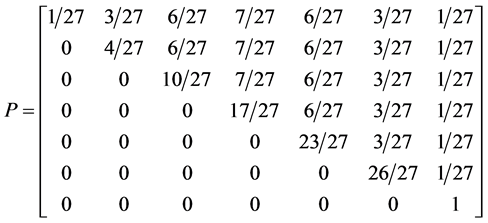
<?xml version="1.0" encoding="UTF-8"?><!DOCTYPE article  PUBLIC "-//NLM//DTD Journal Publishing DTD v3.0 20080202//EN" "http://dtd.nlm.nih.gov/publishing/3.0/journalpublishing3.dtd"><article xmlns:mml="http://www.w3.org/1998/Math/MathML" xmlns:xlink="http://www.w3.org/1999/xlink" dtd-version="3.0" xml:lang="en" article-type="research article"><front><journal-meta><journal-id journal-id-type="publisher-id">AM</journal-id><journal-title-group><journal-title>Applied Mathematics</journal-title></journal-title-group><issn pub-type="epub">2152-7385</issn><publisher><publisher-name>Scientific Research Publishing</publisher-name></publisher></journal-meta><article-meta><article-id pub-id-type="doi">10.4236/am.2016.77060</article-id><article-id pub-id-type="publisher-id">AM-66038</article-id><article-categories><subj-group subj-group-type="heading"><subject>Articles</subject></subj-group><subj-group subj-group-type="Discipline-v2"><subject>Physics&amp;Mathematics</subject></subj-group></article-categories><title-group><article-title>
 
 
  Energy-States of Particles with Representational Spin
 
</article-title></title-group><contrib-group><contrib contrib-type="author" xlink:type="simple"><name name-style="western"><surname>icardo</surname><given-names>Suarez</given-names></name><xref ref-type="aff" rid="aff1"><sup>1</sup></xref></contrib><contrib contrib-type="author" xlink:type="simple"><name name-style="western"><surname>Gregory</surname><given-names>G. Wood</given-names></name><xref ref-type="aff" rid="aff2"><sup>2</sup></xref></contrib></contrib-group><aff id="aff1"><addr-line>Department of Mathematics, CSU Channel Islands, Camarillo, CA, USA</addr-line></aff><aff id="aff2"><addr-line>Department of Physics, CSU Channel Islands, Camarillo, CA, USA</addr-line></aff><pub-date pub-type="epub"><day>18</day><month>04</month><year>2016</year></pub-date><volume>07</volume><issue>07</issue><fpage>650</fpage><lpage>664</lpage><history><date date-type="received"><day>7</day>	<month>March</month>	<year>2016</year></date><date date-type="rev-recd"><day>accepted</day>	<month>25</month>	<year>April</year>	</date><date date-type="accepted"><day>28</day>	<month>April</month>	<year>2016</year></date></history><permissions><copyright-statement>&#169; Copyright  2014 by authors and Scientific Research Publishing Inc. </copyright-statement><copyright-year>2014</copyright-year><license><license-p>This work is licensed under the Creative Commons Attribution International License (CC BY). http://creativecommons.org/licenses/by/4.0/</license-p></license></permissions><abstract><p>
 
 
  In this paper, an algorithm to produce a transition matrix between all states in ideal anti-paramagetic system under the simulated annealing condition that only moves to lower energy states are accepted. The check the accuracy of the transition matrix is confirmed by computer simulation, showing close agreement between model and simulation results.
 
</p></abstract><kwd-group><kwd>Markov Chain Monte Carlo</kwd><kwd> Simulated Annealing</kwd><kwd> Spin 1/2 Particles</kwd></kwd-group></article-meta></front><body><sec id="s1"><title>1. Introduction</title><p>In this paper we compute all transition probabilities of a system of N isolated particles of spin M to move to any lower energy state. In each move, the current state<inline-formula><inline-graphic xlink:href="http://html.scirp.org/file/8-7403118x6.png" xlink:type="simple"/></inline-formula>, is compared with a random trial state,<inline-formula><inline-graphic xlink:href="http://html.scirp.org/file/8-7403118x7.png" xlink:type="simple"/></inline-formula>. The move is accepted if it the trial state has a lower energy, and rejected if the energy is equal, or higher. No restrictions are placed upon the trial state: it is totally random, thus the states form a Markov chain [<xref ref-type="bibr" rid="scirp.66038-ref1">1</xref>] which the next state chosen at random, via the Monte Carlo method [<xref ref-type="bibr" rid="scirp.66038-ref2">2</xref>] . This is a kind of simulated annealing [<xref ref-type="bibr" rid="scirp.66038-ref3">3</xref>] , but with a simulation temperature of zero [<xref ref-type="bibr" rid="scirp.66038-ref4">4</xref>] , which continues to be relevant within the context of recent work [<xref ref-type="bibr" rid="scirp.66038-ref5">5</xref>] . The system will approach its idealized energy state, with net magnetic moment <inline-formula><inline-graphic xlink:href="http://html.scirp.org/file/8-7403118x8.png" xlink:type="simple"/></inline-formula> , where <inline-formula><inline-graphic xlink:href="http://html.scirp.org/file/8-7403118x9.png" xlink:type="simple"/></inline-formula> is the magnetic moment of one particle, with energy<inline-formula><inline-graphic xlink:href="http://html.scirp.org/file/8-7403118x10.png" xlink:type="simple"/></inline-formula>, with entropy<inline-formula><inline-graphic xlink:href="http://html.scirp.org/file/8-7403118x11.png" xlink:type="simple"/></inline-formula>. For the context of this paper, we will consider the system to be an diamagnet, with the external magnetic field pointing up, the ground state (lowest energy) for the system will be when all spins point down.The least preferred state will be the state that has all spins up. Results are essentially the same for paramagnetic systems, but with the transition matrix is the flipped.</p><p>This is an unusual use of simulated annealing. Normally, simulated annealing is used to find a solution to a complex problem, such as the optimal path in the traveling salesman problem. In complex magnetic systems, such as spin glasses, simulated annealing is used to find the optimal ground state [<xref ref-type="bibr" rid="scirp.66038-ref6">6</xref>] . By contrast, in this paper, the system is rather simple and the optimal state is known. Thus we can compute the probability to move from any state to any other state which should lend insight into how this very powerful tool (simulated annealing) operates. We can pause the simulation at any point, and since we know the optimal state, measure how far the system is from optimal, The number of moves to find the best state increases rapidly with the complexity of the system. In the magnetic systems we study in this paper, this complexity can be increased by increasing the number of spins in the system, or by increasing the spin of each particle. Either way greatly increases the number of states for the system to explore.</p><sec id="s1_1"><title>1.1. Plan of the Paper</title><p>Beginning with two, three and four spin one half particle states, the transition probabilities between all states are enumerated. These lists of probabilities are formed into matrices. This is repeated for spin one particles in section 2 where the transition probabilities are derived from the degeneracy of the states. These degeneracies employ the generalized binomial coefficients, called the multinomials. In Section 3, the spin 3/2 particles are considered. Then, in Section 4, the entries in the transition matrices are derived from the degeneracy of the states, using a simple summation rule. In Section 5, degeneracy vectors are given for various systems. In Section 6, the results of numerical simulations are provided which confirm the results of the matrix calculations.</p></sec><sec id="s1_2"><title>1.2. Assumptions of Model</title><p>Our underlying assumptions are:</p><p>・ <inline-formula><inline-graphic xlink:href="http://html.scirp.org/file/8-7403118x12.png" xlink:type="simple"/></inline-formula>, thus eliminating the effects of entropy <inline-formula><inline-graphic xlink:href="http://html.scirp.org/file/8-7403118x13.png" xlink:type="simple"/></inline-formula></p><p>・ <inline-formula><inline-graphic xlink:href="http://html.scirp.org/file/8-7403118x14.png" xlink:type="simple"/></inline-formula>states gravitate towards more preferred states of lower magnetism number due to our model being an anti-paramagnet</p><p>・ Particles in <inline-formula><inline-graphic xlink:href="http://html.scirp.org/file/8-7403118x15.png" xlink:type="simple"/></inline-formula> are indistinguishable.</p><p>In any system N-particles with spin we will assign values. Those values will be relative to the system we are working with. We will assign +1 for spin up, and values −1 for spin down in a spin one half system. +1, 0, −1 for a spin one system, and<inline-formula><inline-graphic xlink:href="http://html.scirp.org/file/8-7403118x16.png" xlink:type="simple"/></inline-formula>, <inline-formula><inline-graphic xlink:href="http://html.scirp.org/file/8-7403118x17.png" xlink:type="simple"/></inline-formula>for a spin 3/2 system. The magnetism number will be achieved by virtue of the magnetism operator S.</p><p>Definition 1.1. For any state <inline-formula><inline-graphic xlink:href="http://html.scirp.org/file/8-7403118x18.png" xlink:type="simple"/></inline-formula> in a N-particle system we define S to be the operator such that <inline-formula><inline-graphic xlink:href="http://html.scirp.org/file/8-7403118x19.png" xlink:type="simple"/></inline-formula> where <inline-formula><inline-graphic xlink:href="http://html.scirp.org/file/8-7403118x20.png" xlink:type="simple"/></inline-formula> is the total spin up, <inline-formula><inline-graphic xlink:href="http://html.scirp.org/file/8-7403118x20.png" xlink:type="simple"/></inline-formula><inline-formula><inline-graphic xlink:href="http://html.scirp.org/file/8-7403118x21.png" xlink:type="simple"/></inline-formula>Total spin down.</p><p>Definition 1.2. For any two states<inline-formula><inline-graphic xlink:href="http://html.scirp.org/file/8-7403118x22.png" xlink:type="simple"/></inline-formula>, <inline-formula><inline-graphic xlink:href="http://html.scirp.org/file/8-7403118x22.png" xlink:type="simple"/></inline-formula><inline-formula><inline-graphic xlink:href="http://html.scirp.org/file/8-7403118x23.png" xlink:type="simple"/></inline-formula>with<inline-formula><inline-graphic xlink:href="http://html.scirp.org/file/8-7403118x22.png" xlink:type="simple"/></inline-formula><inline-formula><inline-graphic xlink:href="http://html.scirp.org/file/8-7403118x23.png" xlink:type="simple"/></inline-formula><inline-formula><inline-graphic xlink:href="http://html.scirp.org/file/8-7403118x24.png" xlink:type="simple"/></inline-formula>, <inline-formula><inline-graphic xlink:href="http://html.scirp.org/file/8-7403118x22.png" xlink:type="simple"/></inline-formula><inline-formula><inline-graphic xlink:href="http://html.scirp.org/file/8-7403118x23.png" xlink:type="simple"/></inline-formula><inline-formula><inline-graphic xlink:href="http://html.scirp.org/file/8-7403118x24.png" xlink:type="simple"/></inline-formula><inline-formula><inline-graphic xlink:href="http://html.scirp.org/file/8-7403118x25.png" xlink:type="simple"/></inline-formula>we say <inline-formula><inline-graphic xlink:href="http://html.scirp.org/file/8-7403118x22.png" xlink:type="simple"/></inline-formula><inline-formula><inline-graphic xlink:href="http://html.scirp.org/file/8-7403118x23.png" xlink:type="simple"/></inline-formula><inline-formula><inline-graphic xlink:href="http://html.scirp.org/file/8-7403118x24.png" xlink:type="simple"/></inline-formula><inline-formula><inline-graphic xlink:href="http://html.scirp.org/file/8-7403118x25.png" xlink:type="simple"/></inline-formula><inline-formula><inline-graphic xlink:href="http://html.scirp.org/file/8-7403118x26.png" xlink:type="simple"/></inline-formula> is preferred to <inline-formula><inline-graphic xlink:href="http://html.scirp.org/file/8-7403118x22.png" xlink:type="simple"/></inline-formula><inline-formula><inline-graphic xlink:href="http://html.scirp.org/file/8-7403118x23.png" xlink:type="simple"/></inline-formula><inline-formula><inline-graphic xlink:href="http://html.scirp.org/file/8-7403118x24.png" xlink:type="simple"/></inline-formula><inline-formula><inline-graphic xlink:href="http://html.scirp.org/file/8-7403118x25.png" xlink:type="simple"/></inline-formula><inline-formula><inline-graphic xlink:href="http://html.scirp.org/file/8-7403118x26.png" xlink:type="simple"/></inline-formula><inline-formula><inline-graphic xlink:href="http://html.scirp.org/file/8-7403118x27.png" xlink:type="simple"/></inline-formula> iff<inline-formula><inline-graphic xlink:href="http://html.scirp.org/file/8-7403118x22.png" xlink:type="simple"/></inline-formula><inline-formula><inline-graphic xlink:href="http://html.scirp.org/file/8-7403118x23.png" xlink:type="simple"/></inline-formula><inline-formula><inline-graphic xlink:href="http://html.scirp.org/file/8-7403118x24.png" xlink:type="simple"/></inline-formula><inline-formula><inline-graphic xlink:href="http://html.scirp.org/file/8-7403118x25.png" xlink:type="simple"/></inline-formula><inline-formula><inline-graphic xlink:href="http://html.scirp.org/file/8-7403118x26.png" xlink:type="simple"/></inline-formula><inline-formula><inline-graphic xlink:href="http://html.scirp.org/file/8-7403118x27.png" xlink:type="simple"/></inline-formula><inline-formula><inline-graphic xlink:href="http://html.scirp.org/file/8-7403118x28.png" xlink:type="simple"/></inline-formula>.</p><p>Definition 1.3. For any N-particle system. <inline-formula><inline-graphic xlink:href="http://html.scirp.org/file/8-7403118x29.png" xlink:type="simple"/></inline-formula>will be the idealized ground state iff <inline-formula><inline-graphic xlink:href="http://html.scirp.org/file/8-7403118x29.png" xlink:type="simple"/></inline-formula><inline-formula><inline-graphic xlink:href="http://html.scirp.org/file/8-7403118x30.png" xlink:type="simple"/></inline-formula></p><p>Definition 1.4. let <inline-formula><inline-graphic xlink:href="http://html.scirp.org/file/8-7403118x31.png" xlink:type="simple"/></inline-formula> be defined as the set <inline-formula><inline-graphic xlink:href="http://html.scirp.org/file/8-7403118x31.png" xlink:type="simple"/></inline-formula><inline-formula><inline-graphic xlink:href="http://html.scirp.org/file/8-7403118x32.png" xlink:type="simple"/></inline-formula></p><p>Definition 1.5. The cardinality of the set<inline-formula><inline-graphic xlink:href="http://html.scirp.org/file/8-7403118x33.png" xlink:type="simple"/></inline-formula>, denoted <inline-formula><inline-graphic xlink:href="http://html.scirp.org/file/8-7403118x33.png" xlink:type="simple"/></inline-formula><inline-formula><inline-graphic xlink:href="http://html.scirp.org/file/8-7403118x34.png" xlink:type="simple"/></inline-formula> is the total number of states with magnetism number n.</p><p>This leads us to the following proposition.</p><p>Proposition 1.6. There can only be one idealized Ground state;</p><p>that is <inline-formula><inline-graphic xlink:href="http://html.scirp.org/file/8-7403118x35.png" xlink:type="simple"/></inline-formula></p><p>Poof. The only way to get magnetism number <inline-formula><inline-graphic xlink:href="http://html.scirp.org/file/8-7403118x36.png" xlink:type="simple"/></inline-formula> for an N-particle system, is to have all the particles in that system be spin down. Since particles are indistinguishable by assumption 3, there is only one state that gives magnetism number<inline-formula><inline-graphic xlink:href="http://html.scirp.org/file/8-7403118x36.png" xlink:type="simple"/></inline-formula><inline-formula><inline-graphic xlink:href="http://html.scirp.org/file/8-7403118x37.png" xlink:type="simple"/></inline-formula>, thus <inline-formula><inline-graphic xlink:href="http://html.scirp.org/file/8-7403118x36.png" xlink:type="simple"/></inline-formula><inline-formula><inline-graphic xlink:href="http://html.scirp.org/file/8-7403118x37.png" xlink:type="simple"/></inline-formula><inline-formula><inline-graphic xlink:href="http://html.scirp.org/file/8-7403118x38.png" xlink:type="simple"/></inline-formula></p><p>Definition 1.7. let <inline-formula><inline-graphic xlink:href="http://html.scirp.org/file/8-7403118x39.png" xlink:type="simple"/></inline-formula> denote a preferred state to <inline-formula><inline-graphic xlink:href="http://html.scirp.org/file/8-7403118x39.png" xlink:type="simple"/></inline-formula><inline-formula><inline-graphic xlink:href="http://html.scirp.org/file/8-7403118x40.png" xlink:type="simple"/></inline-formula> then</p><disp-formula id="scirp.66038-formula4229"><graphic  xlink:href="http://html.scirp.org/file/8-7403118x41.png"  xlink:type="simple"/></disp-formula><p>is the set of all states that are preferred to a state with magnetism number <inline-formula><inline-graphic xlink:href="http://html.scirp.org/file/8-7403118x42.png" xlink:type="simple"/></inline-formula></p></sec><sec id="s1_3"><title>1.3. Markov Chains</title><p>Definition 1.8. A system with a finite or countably infinite number of states with the property that given a present state, past states have no influence on the future is known as a Markov chain</p><p>Definition 1.9. Markov chains have the property that for a random variable<inline-formula><inline-graphic xlink:href="http://html.scirp.org/file/8-7403118x43.png" xlink:type="simple"/></inline-formula>,</p><disp-formula id="scirp.66038-formula4230"><graphic  xlink:href="http://html.scirp.org/file/8-7403118x44.png"  xlink:type="simple"/></disp-formula><p>where <inline-formula><inline-graphic xlink:href="http://html.scirp.org/file/8-7403118x45.png" xlink:type="simple"/></inline-formula> are in the state space .This property is known as the Markov property.</p><p>Definition 1.10. Let <inline-formula><inline-graphic xlink:href="http://html.scirp.org/file/8-7403118x46.png" xlink:type="simple"/></inline-formula> be in the state space. The conditional probabilities <inline-formula><inline-graphic xlink:href="http://html.scirp.org/file/8-7403118x46.png" xlink:type="simple"/></inline-formula><inline-formula><inline-graphic xlink:href="http://html.scirp.org/file/8-7403118x47.png" xlink:type="simple"/></inline-formula> are known as transition probabilities of the the Markov chain. The function <inline-formula><inline-graphic xlink:href="http://html.scirp.org/file/8-7403118x46.png" xlink:type="simple"/></inline-formula><inline-formula><inline-graphic xlink:href="http://html.scirp.org/file/8-7403118x47.png" xlink:type="simple"/></inline-formula><inline-formula><inline-graphic xlink:href="http://html.scirp.org/file/8-7403118x48.png" xlink:type="simple"/></inline-formula> for any <inline-formula><inline-graphic xlink:href="http://html.scirp.org/file/8-7403118x46.png" xlink:type="simple"/></inline-formula><inline-formula><inline-graphic xlink:href="http://html.scirp.org/file/8-7403118x47.png" xlink:type="simple"/></inline-formula><inline-formula><inline-graphic xlink:href="http://html.scirp.org/file/8-7403118x48.png" xlink:type="simple"/></inline-formula><inline-formula><inline-graphic xlink:href="http://html.scirp.org/file/8-7403118x49.png" xlink:type="simple"/></inline-formula> in the sample space is known as the transition function.</p><p>From the transition function <inline-formula><inline-graphic xlink:href="http://html.scirp.org/file/8-7403118x50.png" xlink:type="simple"/></inline-formula> we construct a square matrix of the form</p><disp-formula id="scirp.66038-formula4231"><graphic  xlink:href="http://html.scirp.org/file/8-7403118x51.png"  xlink:type="simple"/></disp-formula><p>P is known as the transition matrix for the Markov chain. We will now apply the concepts of a Markov chain directly to our model.</p></sec></sec><sec id="s2"><title>2. Markov Chains and Our Model</title><p>We will use Markov chains to model the transition states for spin 1/2, spin 1, or spin 3/2 particles. For our model of N-spin particles the state space <inline-formula><inline-graphic xlink:href="http://html.scirp.org/file/8-7403118x52.png" xlink:type="simple"/></inline-formula> will be composed of all <inline-formula><inline-graphic xlink:href="http://html.scirp.org/file/8-7403118x52.png" xlink:type="simple"/></inline-formula><inline-formula><inline-graphic xlink:href="http://html.scirp.org/file/8-7403118x53.png" xlink:type="simple"/></inline-formula> with different magnetism numbers.</p><p>We begin by defining the probability function for our model.</p><p>Definition 2.1. Let <inline-formula><inline-graphic xlink:href="http://html.scirp.org/file/8-7403118x54.png" xlink:type="simple"/></inline-formula> be the probability of being on a state <inline-formula><inline-graphic xlink:href="http://html.scirp.org/file/8-7403118x54.png" xlink:type="simple"/></inline-formula><inline-formula><inline-graphic xlink:href="http://html.scirp.org/file/8-7403118x55.png" xlink:type="simple"/></inline-formula> such that<inline-formula><inline-graphic xlink:href="http://html.scirp.org/file/8-7403118x54.png" xlink:type="simple"/></inline-formula><inline-formula><inline-graphic xlink:href="http://html.scirp.org/file/8-7403118x55.png" xlink:type="simple"/></inline-formula><inline-formula><inline-graphic xlink:href="http://html.scirp.org/file/8-7403118x56.png" xlink:type="simple"/></inline-formula>. This probability function is defined as</p><disp-formula id="scirp.66038-formula4232"><graphic  xlink:href="http://html.scirp.org/file/8-7403118x57.png"  xlink:type="simple"/></disp-formula><p>where N is total number of particles in the system,</p><p>and <inline-formula><inline-graphic xlink:href="http://html.scirp.org/file/8-7403118x58.png" xlink:type="simple"/></inline-formula> for spin 1/2, spin 1, spin 3/2 particles respectively.</p><p>Since our Markov chain has the property of only transferring to preferred states, our transition probabilities are defined by the following transition function.</p><disp-formula id="scirp.66038-formula4233"><graphic  xlink:href="http://html.scirp.org/file/8-7403118x59.png"  xlink:type="simple"/></disp-formula><p>This transition function shows how transition probabilities are absorbed when we move to a preferred state from a less desired state. This probability absorption allows us to construct upper triangular square transition matrices of the following form.</p><disp-formula id="scirp.66038-formula4234"><graphic  xlink:href="http://html.scirp.org/file/8-7403118x60.png"  xlink:type="simple"/></disp-formula><p>Our understanding of the transition function and the transition matrix of our model leads to the following 2 propositions .</p><p>Proposition 2.2. <inline-formula><inline-graphic xlink:href="http://html.scirp.org/file/8-7403118x61.png" xlink:type="simple"/></inline-formula></p><p>Poof. Staring with<inline-formula><inline-graphic xlink:href="http://html.scirp.org/file/8-7403118x62.png" xlink:type="simple"/></inline-formula>, we can quickly see that</p><disp-formula id="scirp.66038-formula4235"><graphic  xlink:href="http://html.scirp.org/file/8-7403118x63.png"  xlink:type="simple"/></disp-formula><p>Now <inline-formula><inline-graphic xlink:href="http://html.scirp.org/file/8-7403118x64.png" xlink:type="simple"/></inline-formula> will be the probability of all of the states that are not preferred to<inline-formula><inline-graphic xlink:href="http://html.scirp.org/file/8-7403118x64.png" xlink:type="simple"/></inline-formula><inline-formula><inline-graphic xlink:href="http://html.scirp.org/file/8-7403118x65.png" xlink:type="simple"/></inline-formula>. Thus</p><disp-formula id="scirp.66038-formula4236"><graphic  xlink:href="http://html.scirp.org/file/8-7403118x66.png"  xlink:type="simple"/></disp-formula><p>Giving us the desired result.</p><p>Proposition 2.3. For the idealized ground state <inline-formula><inline-graphic xlink:href="http://html.scirp.org/file/8-7403118x67.png" xlink:type="simple"/></inline-formula></p><p>Poof. By proposition 4.2</p><disp-formula id="scirp.66038-formula4237"><graphic  xlink:href="http://html.scirp.org/file/8-7403118x68.png"  xlink:type="simple"/></disp-formula><p>We will now look at Markov chains and the spin 1/2 particle.</p></sec><sec id="s3"><title>3. Spin 1/2 Particles</title><sec id="s3_1"><title>3.1. Two Spin One Half Particles</title><p>For a two spin one half particles, the only possibilities of spin configuration of the fermions look like this</p><p>・ <inline-formula><inline-graphic xlink:href="http://html.scirp.org/file/8-7403118x69.png" xlink:type="simple"/></inline-formula>, <inline-formula><inline-graphic xlink:href="http://html.scirp.org/file/8-7403118x69.png" xlink:type="simple"/></inline-formula><inline-formula><inline-graphic xlink:href="http://html.scirp.org/file/8-7403118x70.png" xlink:type="simple"/></inline-formula></p><p>・ <inline-formula><inline-graphic xlink:href="http://html.scirp.org/file/8-7403118x71.png" xlink:type="simple"/></inline-formula>,<inline-formula><inline-graphic xlink:href="http://html.scirp.org/file/8-7403118x71.png" xlink:type="simple"/></inline-formula><inline-formula><inline-graphic xlink:href="http://html.scirp.org/file/8-7403118x72.png" xlink:type="simple"/></inline-formula>; <inline-formula><inline-graphic xlink:href="http://html.scirp.org/file/8-7403118x71.png" xlink:type="simple"/></inline-formula><inline-formula><inline-graphic xlink:href="http://html.scirp.org/file/8-7403118x72.png" xlink:type="simple"/></inline-formula><inline-formula><inline-graphic xlink:href="http://html.scirp.org/file/8-7403118x73.png" xlink:type="simple"/></inline-formula></p><p>・ <inline-formula><inline-graphic xlink:href="http://html.scirp.org/file/8-7403118x74.png" xlink:type="simple"/></inline-formula>, <inline-formula><inline-graphic xlink:href="http://html.scirp.org/file/8-7403118x74.png" xlink:type="simple"/></inline-formula><inline-formula><inline-graphic xlink:href="http://html.scirp.org/file/8-7403118x75.png" xlink:type="simple"/></inline-formula></p><p>Thus <inline-formula><inline-graphic xlink:href="http://html.scirp.org/file/8-7403118x76.png" xlink:type="simple"/></inline-formula> make up the state space of the two fermion system with our underlying 3 assumptions.</p><p>Giving us the following probability transition table</p><disp-formula id="scirp.66038-formula4238"><graphic  xlink:href="http://html.scirp.org/file/8-7403118x77.png"  xlink:type="simple"/></disp-formula><p>With transition matrix</p><disp-formula id="scirp.66038-formula4239"><graphic  xlink:href="http://html.scirp.org/file/8-7403118x78.png"  xlink:type="simple"/></disp-formula><p>For example we would read<inline-formula><inline-graphic xlink:href="http://html.scirp.org/file/8-7403118x79.png" xlink:type="simple"/></inline-formula>, and<inline-formula><inline-graphic xlink:href="http://html.scirp.org/file/8-7403118x79.png" xlink:type="simple"/></inline-formula><inline-formula><inline-graphic xlink:href="http://html.scirp.org/file/8-7403118x80.png" xlink:type="simple"/></inline-formula>; it is our assumption 2 that makes all of</p><p>our probability matrices upper triangular. Which for our model denotes that system is probabilistically approaching the idealized ground state. Since read <inline-formula><inline-graphic xlink:href="http://html.scirp.org/file/8-7403118x81.png" xlink:type="simple"/></inline-formula> then <inline-formula><inline-graphic xlink:href="http://html.scirp.org/file/8-7403118x81.png" xlink:type="simple"/></inline-formula><inline-formula><inline-graphic xlink:href="http://html.scirp.org/file/8-7403118x82.png" xlink:type="simple"/></inline-formula> is an absorbing state, physically it shows that it is the idealized ground state.</p></sec><sec id="s3_2"><title>3.2. Three Spin One Half Particles</title><p>For a system of three spin one half particles, the only possibilities of spin configuration of the fermions look like this</p><p>・ <inline-formula><inline-graphic xlink:href="http://html.scirp.org/file/8-7403118x83.png" xlink:type="simple"/></inline-formula></p><p>・ <inline-formula><inline-graphic xlink:href="http://html.scirp.org/file/8-7403118x84.png" xlink:type="simple"/></inline-formula></p><p>・ <inline-formula><inline-graphic xlink:href="http://html.scirp.org/file/8-7403118x85.png" xlink:type="simple"/></inline-formula></p><p>・ <inline-formula><inline-graphic xlink:href="http://html.scirp.org/file/8-7403118x86.png" xlink:type="simple"/></inline-formula></p><p>Thus <inline-formula><inline-graphic xlink:href="http://html.scirp.org/file/8-7403118x87.png" xlink:type="simple"/></inline-formula> make up the state space <inline-formula><inline-graphic xlink:href="http://html.scirp.org/file/8-7403118x87.png" xlink:type="simple"/></inline-formula><inline-formula><inline-graphic xlink:href="http://html.scirp.org/file/8-7403118x88.png" xlink:type="simple"/></inline-formula> of the three fermion system with our underlying 3 assumptions.</p><p>Although we can clearly see what the probability of landing in each state is, we can use basic counting arguments to show our results mathematically. Thus</p><p>・ <inline-formula><inline-graphic xlink:href="http://html.scirp.org/file/8-7403118x89.png" xlink:type="simple"/></inline-formula></p><p>・ <inline-formula><inline-graphic xlink:href="http://html.scirp.org/file/8-7403118x90.png" xlink:type="simple"/></inline-formula></p><p>・ <inline-formula><inline-graphic xlink:href="http://html.scirp.org/file/8-7403118x91.png" xlink:type="simple"/></inline-formula></p><p>・ <inline-formula><inline-graphic xlink:href="http://html.scirp.org/file/8-7403118x92.png" xlink:type="simple"/></inline-formula></p><p>Giving us the following probability transition table</p><disp-formula id="scirp.66038-formula4240"><graphic  xlink:href="http://html.scirp.org/file/8-7403118x93.png"  xlink:type="simple"/></disp-formula><p>With transition marix</p><disp-formula id="scirp.66038-formula4241"><graphic  xlink:href="http://html.scirp.org/file/8-7403118x94.png"  xlink:type="simple"/></disp-formula><p>Example 3.1. Given the transition matrix for the three spin one half particle system, above, we can calculate the probablity of moving to a preferred state.</p><p>・ <inline-formula><inline-graphic xlink:href="http://html.scirp.org/file/8-7403118x95.png" xlink:type="simple"/></inline-formula></p><p>・ <inline-formula><inline-graphic xlink:href="http://html.scirp.org/file/8-7403118x96.png" xlink:type="simple"/></inline-formula></p><p>・ <inline-formula><inline-graphic xlink:href="http://html.scirp.org/file/8-7403118x97.png" xlink:type="simple"/></inline-formula></p><p>・ <inline-formula><inline-graphic xlink:href="http://html.scirp.org/file/8-7403118x98.png" xlink:type="simple"/></inline-formula></p><p>With our understanding of the three spin one half particle case and counting arguments, we can develop a generalization for any N spin one half particle system.</p></sec><sec id="s3_3"><title>3.3. N-Spin One Half Particle System</title><p>Now given our understanding of the probabilities we can build the probability transition matrix for any N-fer- mion system. If <inline-formula><inline-graphic xlink:href="http://html.scirp.org/file/8-7403118x99.png" xlink:type="simple"/></inline-formula> with <inline-formula><inline-graphic xlink:href="http://html.scirp.org/file/8-7403118x99.png" xlink:type="simple"/></inline-formula><inline-formula><inline-graphic xlink:href="http://html.scirp.org/file/8-7403118x100.png" xlink:type="simple"/></inline-formula> our transition matrix looks like this</p><disp-formula id="scirp.66038-formula4242"><graphic  xlink:href="http://html.scirp.org/file/8-7403118x101.png"  xlink:type="simple"/></disp-formula><p>And with <inline-formula><inline-graphic xlink:href="http://html.scirp.org/file/8-7403118x102.png" xlink:type="simple"/></inline-formula> s.t <inline-formula><inline-graphic xlink:href="http://html.scirp.org/file/8-7403118x102.png" xlink:type="simple"/></inline-formula><inline-formula><inline-graphic xlink:href="http://html.scirp.org/file/8-7403118x103.png" xlink:type="simple"/></inline-formula> we get the probability transition matrix</p><disp-formula id="scirp.66038-formula4243"><graphic  xlink:href="http://html.scirp.org/file/8-7403118x104.png"  xlink:type="simple"/></disp-formula><p>Leading us to the following definition.</p><p>Definition 3.2. For any N-fermion system we can calculate <inline-formula><inline-graphic xlink:href="http://html.scirp.org/file/8-7403118x105.png" xlink:type="simple"/></inline-formula> where <inline-formula><inline-graphic xlink:href="http://html.scirp.org/file/8-7403118x105.png" xlink:type="simple"/></inline-formula><inline-formula><inline-graphic xlink:href="http://html.scirp.org/file/8-7403118x106.png" xlink:type="simple"/></inline-formula> is not the idealized ground state. Let <inline-formula><inline-graphic xlink:href="http://html.scirp.org/file/8-7403118x105.png" xlink:type="simple"/></inline-formula><inline-formula><inline-graphic xlink:href="http://html.scirp.org/file/8-7403118x106.png" xlink:type="simple"/></inline-formula><inline-formula><inline-graphic xlink:href="http://html.scirp.org/file/8-7403118x107.png" xlink:type="simple"/></inline-formula> be the number of spin up or spin down particles for magnetism number m. Then</p><disp-formula id="scirp.66038-formula4244"><graphic  xlink:href="http://html.scirp.org/file/8-7403118x108.png"  xlink:type="simple"/></disp-formula><p>Definition 3.3. For any N-fermion system we can calculate <inline-formula><inline-graphic xlink:href="http://html.scirp.org/file/8-7403118x109.png" xlink:type="simple"/></inline-formula> where <inline-formula><inline-graphic xlink:href="http://html.scirp.org/file/8-7403118x109.png" xlink:type="simple"/></inline-formula><inline-formula><inline-graphic xlink:href="http://html.scirp.org/file/8-7403118x110.png" xlink:type="simple"/></inline-formula> is not the idealized ground state.</p><disp-formula id="scirp.66038-formula4245"><graphic  xlink:href="http://html.scirp.org/file/8-7403118x111.png"  xlink:type="simple"/></disp-formula><p>With these result we can calculate the probability of our system moving to a better state, given any N-fer- mions and<inline-formula><inline-graphic xlink:href="http://html.scirp.org/file/8-7403118x112.png" xlink:type="simple"/></inline-formula>. We now turn our attention to systems of spin one particles.</p></sec></sec><sec id="s4"><title>4. Spin One Particles</title><p>For the spin one particles we will assign <inline-formula><inline-graphic xlink:href="http://html.scirp.org/file/8-7403118x113.png" xlink:type="simple"/></inline-formula> for <inline-formula><inline-graphic xlink:href="http://html.scirp.org/file/8-7403118x113.png" xlink:type="simple"/></inline-formula><inline-formula><inline-graphic xlink:href="http://html.scirp.org/file/8-7403118x114.png" xlink:type="simple"/></inline-formula> respectively. The assumptions to the model will not change. The goal is examine N-spin one systems, and to see how their transition matrices look.</p><sec id="s4_1"><title>4.1. System of Two Spin One Particles</title><p>A system with two spin one particles has the following states:</p><p>・ <inline-formula><inline-graphic xlink:href="http://html.scirp.org/file/8-7403118x115.png" xlink:type="simple"/></inline-formula>, <inline-formula><inline-graphic xlink:href="http://html.scirp.org/file/8-7403118x115.png" xlink:type="simple"/></inline-formula><inline-formula><inline-graphic xlink:href="http://html.scirp.org/file/8-7403118x116.png" xlink:type="simple"/></inline-formula>,</p><p>・ <inline-formula><inline-graphic xlink:href="http://html.scirp.org/file/8-7403118x117.png" xlink:type="simple"/></inline-formula>, <inline-formula><inline-graphic xlink:href="http://html.scirp.org/file/8-7403118x117.png" xlink:type="simple"/></inline-formula><inline-formula><inline-graphic xlink:href="http://html.scirp.org/file/8-7403118x118.png" xlink:type="simple"/></inline-formula></p><p>・ <inline-formula><inline-graphic xlink:href="http://html.scirp.org/file/8-7403118x119.png" xlink:type="simple"/></inline-formula>, <inline-formula><inline-graphic xlink:href="http://html.scirp.org/file/8-7403118x119.png" xlink:type="simple"/></inline-formula><inline-formula><inline-graphic xlink:href="http://html.scirp.org/file/8-7403118x120.png" xlink:type="simple"/></inline-formula>,</p><p>・ <inline-formula><inline-graphic xlink:href="http://html.scirp.org/file/8-7403118x121.png" xlink:type="simple"/></inline-formula>, <inline-formula><inline-graphic xlink:href="http://html.scirp.org/file/8-7403118x121.png" xlink:type="simple"/></inline-formula><inline-formula><inline-graphic xlink:href="http://html.scirp.org/file/8-7403118x122.png" xlink:type="simple"/></inline-formula></p><p>・ <inline-formula><inline-graphic xlink:href="http://html.scirp.org/file/8-7403118x123.png" xlink:type="simple"/></inline-formula>, <inline-formula><inline-graphic xlink:href="http://html.scirp.org/file/8-7403118x123.png" xlink:type="simple"/></inline-formula><inline-formula><inline-graphic xlink:href="http://html.scirp.org/file/8-7403118x124.png" xlink:type="simple"/></inline-formula>,</p><p>・ <inline-formula><inline-graphic xlink:href="http://html.scirp.org/file/8-7403118x125.png" xlink:type="simple"/></inline-formula>, <inline-formula><inline-graphic xlink:href="http://html.scirp.org/file/8-7403118x125.png" xlink:type="simple"/></inline-formula><inline-formula><inline-graphic xlink:href="http://html.scirp.org/file/8-7403118x126.png" xlink:type="simple"/></inline-formula></p><p>・ <inline-formula><inline-graphic xlink:href="http://html.scirp.org/file/8-7403118x127.png" xlink:type="simple"/></inline-formula>, <inline-formula><inline-graphic xlink:href="http://html.scirp.org/file/8-7403118x127.png" xlink:type="simple"/></inline-formula><inline-formula><inline-graphic xlink:href="http://html.scirp.org/file/8-7403118x128.png" xlink:type="simple"/></inline-formula>,</p><p>・ <inline-formula><inline-graphic xlink:href="http://html.scirp.org/file/8-7403118x129.png" xlink:type="simple"/></inline-formula>, <inline-formula><inline-graphic xlink:href="http://html.scirp.org/file/8-7403118x129.png" xlink:type="simple"/></inline-formula><inline-formula><inline-graphic xlink:href="http://html.scirp.org/file/8-7403118x130.png" xlink:type="simple"/></inline-formula></p><p>Thus for a system of two spin one particles, the state space <inline-formula><inline-graphic xlink:href="http://html.scirp.org/file/8-7403118x131.png" xlink:type="simple"/></inline-formula> has possible states<inline-formula><inline-graphic xlink:href="http://html.scirp.org/file/8-7403118x131.png" xlink:type="simple"/></inline-formula><inline-formula><inline-graphic xlink:href="http://html.scirp.org/file/8-7403118x132.png" xlink:type="simple"/></inline-formula>.<inline-formula><inline-graphic xlink:href="http://html.scirp.org/file/8-7403118x131.png" xlink:type="simple"/></inline-formula><inline-formula><inline-graphic xlink:href="http://html.scirp.org/file/8-7403118x132.png" xlink:type="simple"/></inline-formula><inline-formula><inline-graphic xlink:href="http://html.scirp.org/file/8-7403118x133.png" xlink:type="simple"/></inline-formula>,<inline-formula><inline-graphic xlink:href="http://html.scirp.org/file/8-7403118x131.png" xlink:type="simple"/></inline-formula><inline-formula><inline-graphic xlink:href="http://html.scirp.org/file/8-7403118x132.png" xlink:type="simple"/></inline-formula><inline-formula><inline-graphic xlink:href="http://html.scirp.org/file/8-7403118x133.png" xlink:type="simple"/></inline-formula><inline-formula><inline-graphic xlink:href="http://html.scirp.org/file/8-7403118x134.png" xlink:type="simple"/></inline-formula>.<inline-formula><inline-graphic xlink:href="http://html.scirp.org/file/8-7403118x131.png" xlink:type="simple"/></inline-formula><inline-formula><inline-graphic xlink:href="http://html.scirp.org/file/8-7403118x132.png" xlink:type="simple"/></inline-formula><inline-formula><inline-graphic xlink:href="http://html.scirp.org/file/8-7403118x133.png" xlink:type="simple"/></inline-formula><inline-formula><inline-graphic xlink:href="http://html.scirp.org/file/8-7403118x134.png" xlink:type="simple"/></inline-formula><inline-formula><inline-graphic xlink:href="http://html.scirp.org/file/8-7403118x135.png" xlink:type="simple"/></inline-formula>, <inline-formula><inline-graphic xlink:href="http://html.scirp.org/file/8-7403118x131.png" xlink:type="simple"/></inline-formula><inline-formula><inline-graphic xlink:href="http://html.scirp.org/file/8-7403118x132.png" xlink:type="simple"/></inline-formula><inline-formula><inline-graphic xlink:href="http://html.scirp.org/file/8-7403118x133.png" xlink:type="simple"/></inline-formula><inline-formula><inline-graphic xlink:href="http://html.scirp.org/file/8-7403118x134.png" xlink:type="simple"/></inline-formula><inline-formula><inline-graphic xlink:href="http://html.scirp.org/file/8-7403118x135.png" xlink:type="simple"/></inline-formula><inline-formula><inline-graphic xlink:href="http://html.scirp.org/file/8-7403118x136.png" xlink:type="simple"/></inline-formula>, which give us the following transition table</p><disp-formula id="scirp.66038-formula4246"><graphic  xlink:href="http://html.scirp.org/file/8-7403118x137.png"  xlink:type="simple"/></disp-formula><p>With the following transition matrix</p><disp-formula id="scirp.66038-formula4247"><graphic  xlink:href="http://html.scirp.org/file/8-7403118x138.png"  xlink:type="simple"/></disp-formula></sec><sec id="s4_2"><title>4.2. System of Three Spin One Particles</title><p>For a system of three spin one particles the possible states are given by the macro-states<inline-formula><inline-graphic xlink:href="http://html.scirp.org/file/8-7403118x139.png" xlink:type="simple"/></inline-formula>,<inline-formula><inline-graphic xlink:href="http://html.scirp.org/file/8-7403118x139.png" xlink:type="simple"/></inline-formula><inline-formula><inline-graphic xlink:href="http://html.scirp.org/file/8-7403118x140.png" xlink:type="simple"/></inline-formula>.<inline-formula><inline-graphic xlink:href="http://html.scirp.org/file/8-7403118x139.png" xlink:type="simple"/></inline-formula><inline-formula><inline-graphic xlink:href="http://html.scirp.org/file/8-7403118x140.png" xlink:type="simple"/></inline-formula><inline-formula><inline-graphic xlink:href="http://html.scirp.org/file/8-7403118x141.png" xlink:type="simple"/></inline-formula>,<inline-formula><inline-graphic xlink:href="http://html.scirp.org/file/8-7403118x139.png" xlink:type="simple"/></inline-formula><inline-formula><inline-graphic xlink:href="http://html.scirp.org/file/8-7403118x140.png" xlink:type="simple"/></inline-formula><inline-formula><inline-graphic xlink:href="http://html.scirp.org/file/8-7403118x141.png" xlink:type="simple"/></inline-formula><inline-formula><inline-graphic xlink:href="http://html.scirp.org/file/8-7403118x142.png" xlink:type="simple"/></inline-formula>.<inline-formula><inline-graphic xlink:href="http://html.scirp.org/file/8-7403118x139.png" xlink:type="simple"/></inline-formula><inline-formula><inline-graphic xlink:href="http://html.scirp.org/file/8-7403118x140.png" xlink:type="simple"/></inline-formula><inline-formula><inline-graphic xlink:href="http://html.scirp.org/file/8-7403118x141.png" xlink:type="simple"/></inline-formula><inline-formula><inline-graphic xlink:href="http://html.scirp.org/file/8-7403118x142.png" xlink:type="simple"/></inline-formula><inline-formula><inline-graphic xlink:href="http://html.scirp.org/file/8-7403118x143.png" xlink:type="simple"/></inline-formula>, <inline-formula><inline-graphic xlink:href="http://html.scirp.org/file/8-7403118x139.png" xlink:type="simple"/></inline-formula><inline-formula><inline-graphic xlink:href="http://html.scirp.org/file/8-7403118x140.png" xlink:type="simple"/></inline-formula><inline-formula><inline-graphic xlink:href="http://html.scirp.org/file/8-7403118x141.png" xlink:type="simple"/></inline-formula><inline-formula><inline-graphic xlink:href="http://html.scirp.org/file/8-7403118x142.png" xlink:type="simple"/></inline-formula><inline-formula><inline-graphic xlink:href="http://html.scirp.org/file/8-7403118x143.png" xlink:type="simple"/></inline-formula><inline-formula><inline-graphic xlink:href="http://html.scirp.org/file/8-7403118x144.png" xlink:type="simple"/></inline-formula>,<inline-formula><inline-graphic xlink:href="http://html.scirp.org/file/8-7403118x139.png" xlink:type="simple"/></inline-formula><inline-formula><inline-graphic xlink:href="http://html.scirp.org/file/8-7403118x140.png" xlink:type="simple"/></inline-formula><inline-formula><inline-graphic xlink:href="http://html.scirp.org/file/8-7403118x141.png" xlink:type="simple"/></inline-formula><inline-formula><inline-graphic xlink:href="http://html.scirp.org/file/8-7403118x142.png" xlink:type="simple"/></inline-formula><inline-formula><inline-graphic xlink:href="http://html.scirp.org/file/8-7403118x143.png" xlink:type="simple"/></inline-formula><inline-formula><inline-graphic xlink:href="http://html.scirp.org/file/8-7403118x144.png" xlink:type="simple"/></inline-formula><inline-formula><inline-graphic xlink:href="http://html.scirp.org/file/8-7403118x145.png" xlink:type="simple"/></inline-formula>. Whose micro-state configuration looks like this.</p><p>・ <inline-formula><inline-graphic xlink:href="http://html.scirp.org/file/8-7403118x146.png" xlink:type="simple"/></inline-formula></p><p>・ <inline-formula><inline-graphic xlink:href="http://html.scirp.org/file/8-7403118x147.png" xlink:type="simple"/></inline-formula></p><p>・ <inline-formula><inline-graphic xlink:href="http://html.scirp.org/file/8-7403118x148.png" xlink:type="simple"/></inline-formula></p><p>・ <inline-formula><inline-graphic xlink:href="http://html.scirp.org/file/8-7403118x149.png" xlink:type="simple"/></inline-formula></p><p>・ <inline-formula><inline-graphic xlink:href="http://html.scirp.org/file/8-7403118x150.png" xlink:type="simple"/></inline-formula></p><p>・ <inline-formula><inline-graphic xlink:href="http://html.scirp.org/file/8-7403118x151.png" xlink:type="simple"/></inline-formula></p><p>・ <inline-formula><inline-graphic xlink:href="http://html.scirp.org/file/8-7403118x152.png" xlink:type="simple"/></inline-formula></p><p>Thus in terms of probabilities:</p><disp-formula id="scirp.66038-formula4248"><graphic  xlink:href="http://html.scirp.org/file/8-7403118x153.png"  xlink:type="simple"/></disp-formula><disp-formula id="scirp.66038-formula4249"><graphic  xlink:href="http://html.scirp.org/file/8-7403118x154.png"  xlink:type="simple"/></disp-formula><disp-formula id="scirp.66038-formula4250"><graphic  xlink:href="http://html.scirp.org/file/8-7403118x155.png"  xlink:type="simple"/></disp-formula><disp-formula id="scirp.66038-formula4251"><graphic  xlink:href="http://html.scirp.org/file/8-7403118x156.png"  xlink:type="simple"/></disp-formula><p>These probabilities give us the following transition table.</p><disp-formula id="scirp.66038-formula4252"><graphic  xlink:href="http://html.scirp.org/file/8-7403118x157.png"  xlink:type="simple"/></disp-formula><p>With the following transition matrix.</p><p><img data-original="http://html.scirp.org/file/8-7403118x159.png" /><img data-original="http://html.scirp.org/file/8-7403118x158.png" /></p><p>Notice that listing out all appropriate micro states gets a bit cumbersome, but unlike the spin 1/2 particles, the spin one particles have 3 possible spins. So to calculate their probabilities with the aid multinomial probability formula.</p><disp-formula id="scirp.66038-formula4253"><graphic  xlink:href="http://html.scirp.org/file/8-7403118x160.png"  xlink:type="simple"/></disp-formula><p>Now with this formula we are able to calculate the probability of the macro states for a 4 spin one particle system.</p></sec><sec id="s4_3"><title>4.3. 4 Spin One Particle System</title><p>For a spin one system with 4 particles we find macro states <inline-formula><inline-graphic xlink:href="http://html.scirp.org/file/8-7403118x161.png" xlink:type="simple"/></inline-formula> such that<inline-formula><inline-graphic xlink:href="http://html.scirp.org/file/8-7403118x161.png" xlink:type="simple"/></inline-formula><inline-formula><inline-graphic xlink:href="http://html.scirp.org/file/8-7403118x162.png" xlink:type="simple"/></inline-formula>. We do this by calculating their degenerate states via the multinomial formula. Giving us the following results:</p><p>・ <inline-formula><inline-graphic xlink:href="http://html.scirp.org/file/8-7403118x163.png" xlink:type="simple"/></inline-formula></p><p>・ <inline-formula><inline-graphic xlink:href="http://html.scirp.org/file/8-7403118x164.png" xlink:type="simple"/></inline-formula></p><p>・ <inline-formula><inline-graphic xlink:href="http://html.scirp.org/file/8-7403118x165.png" xlink:type="simple"/></inline-formula></p><p>・ <inline-formula><inline-graphic xlink:href="http://html.scirp.org/file/8-7403118x166.png" xlink:type="simple"/></inline-formula></p><p>・ <inline-formula><inline-graphic xlink:href="http://html.scirp.org/file/8-7403118x167.png" xlink:type="simple"/></inline-formula></p><p>・ <inline-formula><inline-graphic xlink:href="http://html.scirp.org/file/8-7403118x168.png" xlink:type="simple"/></inline-formula></p><p>・ <inline-formula><inline-graphic xlink:href="http://html.scirp.org/file/8-7403118x169.png" xlink:type="simple"/></inline-formula></p><p>・ <inline-formula><inline-graphic xlink:href="http://html.scirp.org/file/8-7403118x170.png" xlink:type="simple"/></inline-formula></p><p>・ <inline-formula><inline-graphic xlink:href="http://html.scirp.org/file/8-7403118x171.png" xlink:type="simple"/></inline-formula></p><p>Giving us the following Transition table</p><disp-formula id="scirp.66038-formula4254"><graphic  xlink:href="http://html.scirp.org/file/8-7403118x172.png"  xlink:type="simple"/></disp-formula><p>Along with the following transition matrix</p><disp-formula id="scirp.66038-formula4255"><graphic  xlink:href="http://html.scirp.org/file/8-7403118x173.png"  xlink:type="simple"/></disp-formula><p>We now generalize our results with the following formulas</p><p>Definition 4.1. For any N-spin one particle system and a given macro state <inline-formula><inline-graphic xlink:href="http://html.scirp.org/file/8-7403118x174.png" xlink:type="simple"/></inline-formula> s.t. <inline-formula><inline-graphic xlink:href="http://html.scirp.org/file/8-7403118x174.png" xlink:type="simple"/></inline-formula><inline-formula><inline-graphic xlink:href="http://html.scirp.org/file/8-7403118x175.png" xlink:type="simple"/></inline-formula>the following hold.</p><disp-formula id="scirp.66038-formula4256"><graphic  xlink:href="http://html.scirp.org/file/8-7403118x176.png"  xlink:type="simple"/></disp-formula><p>where <inline-formula><inline-graphic xlink:href="http://html.scirp.org/file/8-7403118x177.png" xlink:type="simple"/></inline-formula> is the degeneracies for <inline-formula><inline-graphic xlink:href="http://html.scirp.org/file/8-7403118x177.png" xlink:type="simple"/></inline-formula><inline-formula><inline-graphic xlink:href="http://html.scirp.org/file/8-7403118x178.png" xlink:type="simple"/></inline-formula></p><disp-formula id="scirp.66038-formula4257"><graphic  xlink:href="http://html.scirp.org/file/8-7403118x179.png"  xlink:type="simple"/></disp-formula><p>If n-even m-even, or n-odd m-odd</p><disp-formula id="scirp.66038-formula4258"><graphic  xlink:href="http://html.scirp.org/file/8-7403118x180.png"  xlink:type="simple"/></disp-formula><p>If N-even m-odd, or N-odd m-even</p><p>And for the zero case we get the following.</p><disp-formula id="scirp.66038-formula4259"><graphic  xlink:href="http://html.scirp.org/file/8-7403118x181.png"  xlink:type="simple"/></disp-formula><p>Definition 4.2. Let <inline-formula><inline-graphic xlink:href="http://html.scirp.org/file/8-7403118x182.png" xlink:type="simple"/></inline-formula> be a macro state, for any N spin one particle system, then the probability of moving to a preferred state is</p><disp-formula id="scirp.66038-formula4260"><graphic  xlink:href="http://html.scirp.org/file/8-7403118x183.png"  xlink:type="simple"/></disp-formula><p>Now with this result we can calculate the probability of our system moving to a preferred state, given N-spin one particles and<inline-formula><inline-graphic xlink:href="http://html.scirp.org/file/8-7403118x184.png" xlink:type="simple"/></inline-formula>.</p><p>We now turn our attention to a system of spin 3/2 particles.</p></sec></sec><sec id="s5"><title>5. Spin 3/2 Particles</title><p>Now we turn our attention to spin 3/2 particles. We will de-note all the possible states a particle can take with</p><p>the set<inline-formula><inline-graphic xlink:href="http://html.scirp.org/file/8-7403118x185.png" xlink:type="simple"/></inline-formula>.</p><p>To give the spin 3/2 particles integer coefficients we simply represent them in the set<inline-formula><inline-graphic xlink:href="http://html.scirp.org/file/8-7403118x186.png" xlink:type="simple"/></inline-formula>. Once again we will hold the assumptions as the spin 1/2, and spin 1 cases to find the Probability transition matrix between macro states.</p><sec id="s5_1"><title>5.1. Two Spin 3/2 Particle System</title><p>A two spin 3/2 particle system has the following states</p><p>・ +3, +3 <inline-formula><inline-graphic xlink:href="http://html.scirp.org/file/8-7403118x187.png" xlink:type="simple"/></inline-formula></p><p>・ +3, +1 <inline-formula><inline-graphic xlink:href="http://html.scirp.org/file/8-7403118x188.png" xlink:type="simple"/></inline-formula></p><p>・ +3, −1 <inline-formula><inline-graphic xlink:href="http://html.scirp.org/file/8-7403118x189.png" xlink:type="simple"/></inline-formula></p><p>・ +3, −3 <inline-formula><inline-graphic xlink:href="http://html.scirp.org/file/8-7403118x190.png" xlink:type="simple"/></inline-formula></p><p>・ +1, +3 <inline-formula><inline-graphic xlink:href="http://html.scirp.org/file/8-7403118x191.png" xlink:type="simple"/></inline-formula></p><p>・ +1, +1 <inline-formula><inline-graphic xlink:href="http://html.scirp.org/file/8-7403118x192.png" xlink:type="simple"/></inline-formula></p><p>・ +1, −1 <inline-formula><inline-graphic xlink:href="http://html.scirp.org/file/8-7403118x193.png" xlink:type="simple"/></inline-formula></p><p>・ +1, −3 <inline-formula><inline-graphic xlink:href="http://html.scirp.org/file/8-7403118x194.png" xlink:type="simple"/></inline-formula></p><p>・ −1, +3 <inline-formula><inline-graphic xlink:href="http://html.scirp.org/file/8-7403118x195.png" xlink:type="simple"/></inline-formula></p><p>・ −1, +1 <inline-formula><inline-graphic xlink:href="http://html.scirp.org/file/8-7403118x196.png" xlink:type="simple"/></inline-formula></p><p>・ −1, −1 <inline-formula><inline-graphic xlink:href="http://html.scirp.org/file/8-7403118x197.png" xlink:type="simple"/></inline-formula></p><p>・ −1, −3 <inline-formula><inline-graphic xlink:href="http://html.scirp.org/file/8-7403118x198.png" xlink:type="simple"/></inline-formula></p><p>・ −3, +3 <inline-formula><inline-graphic xlink:href="http://html.scirp.org/file/8-7403118x199.png" xlink:type="simple"/></inline-formula></p><p>・ −3, +1 <inline-formula><inline-graphic xlink:href="http://html.scirp.org/file/8-7403118x200.png" xlink:type="simple"/></inline-formula></p><p>・ −3, −1 <inline-formula><inline-graphic xlink:href="http://html.scirp.org/file/8-7403118x201.png" xlink:type="simple"/></inline-formula></p><p>・ −3, −3 <inline-formula><inline-graphic xlink:href="http://html.scirp.org/file/8-7403118x202.png" xlink:type="simple"/></inline-formula></p><p>The two particle system gives us the following states <inline-formula><inline-graphic xlink:href="http://html.scirp.org/file/8-7403118x203.png" xlink:type="simple"/></inline-formula> with the pro- babilities ;</p><p>・ <inline-formula><inline-graphic xlink:href="http://html.scirp.org/file/8-7403118x204.png" xlink:type="simple"/></inline-formula></p><p>・ <inline-formula><inline-graphic xlink:href="http://html.scirp.org/file/8-7403118x205.png" xlink:type="simple"/></inline-formula></p><p>・ <inline-formula><inline-graphic xlink:href="http://html.scirp.org/file/8-7403118x206.png" xlink:type="simple"/></inline-formula></p><p>・ <inline-formula><inline-graphic xlink:href="http://html.scirp.org/file/8-7403118x207.png" xlink:type="simple"/></inline-formula></p><p>Giving us the following probability transition table</p><disp-formula id="scirp.66038-formula4261"><graphic  xlink:href="http://html.scirp.org/file/8-7403118x208.png"  xlink:type="simple"/></disp-formula><p>With the following transition matrix</p><disp-formula id="scirp.66038-formula4262"><graphic  xlink:href="http://html.scirp.org/file/8-7403118x209.png"  xlink:type="simple"/></disp-formula></sec><sec id="s5_2"><title>5.2. Three Spin 3/2 Particle System</title><p>For a system of three spin 3/2 particles we calculate the state space in the same manner as we did in the two spin 3/2 particle system. Giving us the following state space <inline-formula><inline-graphic xlink:href="http://html.scirp.org/file/8-7403118x210.png" xlink:type="simple"/></inline-formula></p><p>With the following probabilities:</p><disp-formula id="scirp.66038-formula4263"><graphic  xlink:href="http://html.scirp.org/file/8-7403118x211.png"  xlink:type="simple"/></disp-formula><disp-formula id="scirp.66038-formula4264"><graphic  xlink:href="http://html.scirp.org/file/8-7403118x212.png"  xlink:type="simple"/></disp-formula><disp-formula id="scirp.66038-formula4265"><graphic  xlink:href="http://html.scirp.org/file/8-7403118x213.png"  xlink:type="simple"/></disp-formula><disp-formula id="scirp.66038-formula4266"><graphic  xlink:href="http://html.scirp.org/file/8-7403118x214.png"  xlink:type="simple"/></disp-formula><disp-formula id="scirp.66038-formula4267"><graphic  xlink:href="http://html.scirp.org/file/8-7403118x215.png"  xlink:type="simple"/></disp-formula><p>This results in the following transition table</p><disp-formula id="scirp.66038-formula4268"><graphic  xlink:href="http://html.scirp.org/file/8-7403118x216.png"  xlink:type="simple"/></disp-formula><p>With the following transition matrix</p><disp-formula id="scirp.66038-formula4269"><graphic  xlink:href="http://html.scirp.org/file/8-7403118x217.png"  xlink:type="simple"/></disp-formula></sec><sec id="s5_3"><title>5.3. Four Spin 3/2 Particle System</title><p>With the aid of the multinomial formula we are able to calculate the probabilities of the state space</p><disp-formula id="scirp.66038-formula4270"><graphic  xlink:href="http://html.scirp.org/file/8-7403118x218.png"  xlink:type="simple"/></disp-formula><p>・ <inline-formula><inline-graphic xlink:href="http://html.scirp.org/file/8-7403118x219.png" xlink:type="simple"/></inline-formula></p><p>・ <inline-formula><inline-graphic xlink:href="http://html.scirp.org/file/8-7403118x220.png" xlink:type="simple"/></inline-formula></p><p>・ <inline-formula><inline-graphic xlink:href="http://html.scirp.org/file/8-7403118x221.png" xlink:type="simple"/></inline-formula></p><p>・ <inline-formula><inline-graphic xlink:href="http://html.scirp.org/file/8-7403118x222.png" xlink:type="simple"/></inline-formula></p><p>・ <inline-formula><inline-graphic xlink:href="http://html.scirp.org/file/8-7403118x223.png" xlink:type="simple"/></inline-formula></p><p>・ <inline-formula><inline-graphic xlink:href="http://html.scirp.org/file/8-7403118x224.png" xlink:type="simple"/></inline-formula></p><p>・ <inline-formula><inline-graphic xlink:href="http://html.scirp.org/file/8-7403118x225.png" xlink:type="simple"/></inline-formula></p><p>Which gives us the following degeneracy transition table, with <inline-formula><inline-graphic xlink:href="http://html.scirp.org/file/8-7403118x226.png" xlink:type="simple"/></inline-formula> being the degeneracies for state <inline-formula><inline-graphic xlink:href="http://html.scirp.org/file/8-7403118x226.png" xlink:type="simple"/></inline-formula><inline-formula><inline-graphic xlink:href="http://html.scirp.org/file/8-7403118x227.png" xlink:type="simple"/></inline-formula></p><disp-formula id="scirp.66038-formula4271"><graphic  xlink:href="http://html.scirp.org/file/8-7403118x228.png"  xlink:type="simple"/></disp-formula><p>And the transition matrix</p><disp-formula id="scirp.66038-formula4272"><graphic  xlink:href="http://html.scirp.org/file/8-7403118x229.png"  xlink:type="simple"/></disp-formula><p>With D being the following matrix</p><disp-formula id="scirp.66038-formula4273"><graphic  xlink:href="http://html.scirp.org/file/8-7403118x230.png"  xlink:type="simple"/></disp-formula><p>With D being the degeneracy matrix. Notice that we can construct any transition probability matrix from just understanding degeneracy matrix D. Thus given our systems it suffices to understand degeneracies in order to construct their transition probabilities.</p></sec></sec><sec id="s6"><title>6. Degeneracy Matrix Algorithm</title><p>As we saw in the previous section we can find all the transition probabilities from any j spin-N particle system under assumptions:</p><p>・ <inline-formula><inline-graphic xlink:href="http://html.scirp.org/file/8-7403118x231.png" xlink:type="simple"/></inline-formula>, thus eliminating the effects of entropy <inline-formula><inline-graphic xlink:href="http://html.scirp.org/file/8-7403118x231.png" xlink:type="simple"/></inline-formula><inline-formula><inline-graphic xlink:href="http://html.scirp.org/file/8-7403118x232.png" xlink:type="simple"/></inline-formula></p><p>・ <inline-formula><inline-graphic xlink:href="http://html.scirp.org/file/8-7403118x233.png" xlink:type="simple"/></inline-formula>states gravitate towards more preferred states of lower magnetism number due to our model being an anti-paramagnet</p><p>・ Particles in <inline-formula><inline-graphic xlink:href="http://html.scirp.org/file/8-7403118x234.png" xlink:type="simple"/></inline-formula> are indistinguishable.</p><p>With Probability transition matrix P</p><disp-formula id="scirp.66038-formula4274"><graphic  xlink:href="http://html.scirp.org/file/8-7403118x235.png"  xlink:type="simple"/></disp-formula><p>To construct D let <inline-formula><inline-graphic xlink:href="http://html.scirp.org/file/8-7403118x236.png" xlink:type="simple"/></inline-formula> be the degeneracy vector, composed from all the degeneracies form all the <inline-formula><inline-graphic xlink:href="http://html.scirp.org/file/8-7403118x236.png" xlink:type="simple"/></inline-formula><inline-formula><inline-graphic xlink:href="http://html.scirp.org/file/8-7403118x237.png" xlink:type="simple"/></inline-formula> states</p><disp-formula id="scirp.66038-formula4275"><graphic  xlink:href="http://html.scirp.org/file/8-7403118x238.png"  xlink:type="simple"/></disp-formula><p>With <inline-formula><inline-graphic xlink:href="http://html.scirp.org/file/8-7403118x239.png" xlink:type="simple"/></inline-formula> = number of degeneracies from state <inline-formula><inline-graphic xlink:href="http://html.scirp.org/file/8-7403118x239.png" xlink:type="simple"/></inline-formula><inline-formula><inline-graphic xlink:href="http://html.scirp.org/file/8-7403118x240.png" xlink:type="simple"/></inline-formula> and <inline-formula><inline-graphic xlink:href="http://html.scirp.org/file/8-7403118x239.png" xlink:type="simple"/></inline-formula><inline-formula><inline-graphic xlink:href="http://html.scirp.org/file/8-7403118x240.png" xlink:type="simple"/></inline-formula><inline-formula><inline-graphic xlink:href="http://html.scirp.org/file/8-7403118x241.png" xlink:type="simple"/></inline-formula></p><p>We will now use the degeneracy vector to construct the degeneracy matrix.</p><sec id="s6_1"><title>6.1. Algorithm for Constructing D</title><p>For simplicity we will construct D from our degeneracy vector which we will denote <inline-formula><inline-graphic xlink:href="http://html.scirp.org/file/8-7403118x242.png" xlink:type="simple"/></inline-formula> s.t</p><disp-formula id="scirp.66038-formula4276"><graphic  xlink:href="http://html.scirp.org/file/8-7403118x243.png"  xlink:type="simple"/></disp-formula><p>Thus it follows that <inline-formula><inline-graphic xlink:href="http://html.scirp.org/file/8-7403118x244.png" xlink:type="simple"/></inline-formula></p><p>thus we can rewrite <inline-formula><inline-graphic xlink:href="http://html.scirp.org/file/8-7403118x245.png" xlink:type="simple"/></inline-formula> with</p><disp-formula id="scirp.66038-formula4277"><graphic  xlink:href="http://html.scirp.org/file/8-7403118x246.png"  xlink:type="simple"/></disp-formula><p>Using <inline-formula><inline-graphic xlink:href="http://html.scirp.org/file/8-7403118x247.png" xlink:type="simple"/></inline-formula> as the base for constructing D. We can construct the entire degeneracy matrix D from our degeneracy vector <inline-formula><inline-graphic xlink:href="http://html.scirp.org/file/8-7403118x247.png" xlink:type="simple"/></inline-formula><inline-formula><inline-graphic xlink:href="http://html.scirp.org/file/8-7403118x248.png" xlink:type="simple"/></inline-formula> Now with this generalized algorithm we can construct any degeneracy matrix D, which allows us to construct any probability transition matrix P.</p></sec><sec id="s6_2"><title>6.2. Degeneracy Vector (d<sub>1</sub>) for Spin One Particles for n = 5, 6, 7, 8, 9, 10</title><p>From the preceding section, we see that we can construct the probability transition matrix of a system solely by means of the degeneracy vector. Now here are the degeneracy vectors for n = 5, 6, 7, 8, 9, 10.</p><p>・ for n = 5</p><disp-formula id="scirp.66038-formula4278"><graphic  xlink:href="http://html.scirp.org/file/8-7403118x249.png"  xlink:type="simple"/></disp-formula><p>・ for n = 6</p><disp-formula id="scirp.66038-formula4279"><graphic  xlink:href="http://html.scirp.org/file/8-7403118x250.png"  xlink:type="simple"/></disp-formula><p>・ for n = 7</p><disp-formula id="scirp.66038-formula4280"><graphic  xlink:href="http://html.scirp.org/file/8-7403118x251.png"  xlink:type="simple"/></disp-formula><p>・ for n = 8</p><disp-formula id="scirp.66038-formula4281"><graphic  xlink:href="http://html.scirp.org/file/8-7403118x252.png"  xlink:type="simple"/></disp-formula><p>・ for n = 9</p><disp-formula id="scirp.66038-formula4282"><graphic  xlink:href="http://html.scirp.org/file/8-7403118x253.png"  xlink:type="simple"/></disp-formula><p>・ for n = 10</p><disp-formula id="scirp.66038-formula4283"><graphic  xlink:href="http://html.scirp.org/file/8-7403118x254.png"  xlink:type="simple"/></disp-formula></sec><sec id="s6_3"><title>6.3. Degeneracy Vector (d<sub>1</sub>) for Spin 3/2 Particles for n = 5, 6, 7, 8</title><p>・ for n = 5</p><disp-formula id="scirp.66038-formula4284"><graphic  xlink:href="http://html.scirp.org/file/8-7403118x255.png"  xlink:type="simple"/></disp-formula><p>・ for n = 6</p><disp-formula id="scirp.66038-formula4285"><graphic  xlink:href="http://html.scirp.org/file/8-7403118x256.png"  xlink:type="simple"/></disp-formula><p>・ for n = 7</p><disp-formula id="scirp.66038-formula4286"><graphic  xlink:href="http://html.scirp.org/file/8-7403118x257.png"  xlink:type="simple"/></disp-formula><p>・ for n = 8</p><disp-formula id="scirp.66038-formula4287"><graphic  xlink:href="http://html.scirp.org/file/8-7403118x258.png"  xlink:type="simple"/></disp-formula></sec></sec><sec id="s7"><title>7. Results from Numerical Simulations</title><p>Two systems are studied: a small system with 10 spin 1/2 particles giving 1024 possible states, and a larger system with 20 spin 1/2 particles, with about a million possible states. The system begins in the least optimal state, all spins pointing up, and at each move, a random trial state is generated. If the trial state is more optimal, meaning it has fewer spins pointing up, it is accepted. It is highly probable the first move will be accepted. After many moves, the likelihood of improvement diminishes. We consider three “times” to illustrate the relative movement slowing at large time: after 9, 81 and 729 moves, so the moves are evenly spaced in log time. The simulation is run one million times for the small system, and one hundred thousand times for the large system. The results are displayed in <xref ref-type="fig" rid="fig1">Figure 1</xref> and <xref ref-type="fig" rid="fig2">Figure 2</xref>, and are consistent with the calculation of predicted number at each, as shown in <xref ref-type="table" rid="table1">Table 1</xref> and <xref ref-type="table" rid="table2">Table 2</xref>, below.</p><fig id="fig1"  position="float"><label><xref ref-type="fig" rid="fig1">Figure 1</xref></label><caption><title> Histogram of number of states having various net spin as a function of time. Ten spin one half particles are simulated one million times. The x-axis is the number of spins pointing up, at various times. The y-axis is the number of replicas of the system where this was found, proportional to the probability. Three times are given, in different colors, receding into the page, as: red (9 steps) green (81 time steps) and blue (729 time steps). The distribution is roughly Gaussian, and the distribution moves toward lower numbers of spins pointing up over time, but slowly. Numeric values are given in <xref ref-type="table" rid="table1">Table 1</xref>, along with computed values from the transition matrices from the formula above</title></caption><graphic mimetype="image"   position="float"  xlink:type="simple"  xlink:href="http://html.scirp.org/file/8-7403118x259.png"/></fig><fig id="fig2"  position="float"><label><xref ref-type="fig" rid="fig2">Figure 2</xref></label><caption><title> Histogram of number of states having various net spin as a function of time. The x-axis is the number of spins pointing up. The y-axis is the number of replicas of the system which have the given x-axis value of spins up, and so the y-value is proportional to probability. Twenty spin one half particles are simulated over 729 Monte Carlo steps. One hundred thousand replicas of the system are used. Three times are displayed: after nine steps (red), after 81 steps (green) and after 729 steps (blue). The system has just over one million possible states, and so unlike in figure one, above, 729 steps are not nearly enough to get any significant fraction of the system into the optimal (x-axis value zero) state. However, despite the odds of moving to the optimal state being somewhat worse then one in a million, after only 729 moves, the system is pretty close to optimal: most likely the system has three or four spins pointing up out of 20. Beyond this time, progress is slow</title></caption><graphic mimetype="image"   position="float"  xlink:type="simple"  xlink:href="http://html.scirp.org/file/8-7403118x260.png"/></fig><table-wrap id="table1" ><label><xref ref-type="table" rid="table1">Table 1</xref></label><caption><title> Results from one million replicas of a system of ten spin one half particles. Close agreement is found between simulations and model calculations. Time steps (in the first column) are measured in monte carlo simulation steps. The number of systems, out of a total of one million, in the ground state is given by N<sub>0</sub>, and the number in the first excited state, one spin up, given by N<sub>1</sub>. Columns denoted by sim are from simulated annealing computations, and columns denoted by model are from the model. The simulation results are presented in the first two columns of figure one. Note that all numbers of spins are given in thousands of spins</title></caption><table><tbody><thead><tr><th align="center" valign="middle" >Time</th><th align="center" valign="middle" ><inline-formula><inline-graphic xlink:href="http://html.scirp.org/file/8-7403118x261.png" xlink:type="simple"/></inline-formula>(model) (<inline-formula><inline-graphic xlink:href="http://html.scirp.org/file/8-7403118x262.png" xlink:type="simple"/></inline-formula>)</th><th align="center" valign="middle" ><inline-formula><inline-graphic xlink:href="http://html.scirp.org/file/8-7403118x263.png" xlink:type="simple"/></inline-formula>(sim) (<inline-formula><inline-graphic xlink:href="http://html.scirp.org/file/8-7403118x264.png" xlink:type="simple"/></inline-formula>)</th><th align="center" valign="middle" ><inline-formula><inline-graphic xlink:href="http://html.scirp.org/file/8-7403118x265.png" xlink:type="simple"/></inline-formula>(model) (<inline-formula><inline-graphic xlink:href="http://html.scirp.org/file/8-7403118x266.png" xlink:type="simple"/></inline-formula>)</th><th align="center" valign="middle" ><inline-formula><inline-graphic xlink:href="http://html.scirp.org/file/8-7403118x267.png" xlink:type="simple"/></inline-formula>(sim) (<inline-formula><inline-graphic xlink:href="http://html.scirp.org/file/8-7403118x268.png" xlink:type="simple"/></inline-formula>)</th></tr></thead><tr><td align="center" valign="middle" >9</td><td align="center" valign="middle" >8.75</td><td align="center" valign="middle" >9.50</td><td align="center" valign="middle" >91.7</td><td align="center" valign="middle" >93.1</td></tr><tr><td align="center" valign="middle" >81</td><td align="center" valign="middle" >76.1</td><td align="center" valign="middle" >76.6</td><td align="center" valign="middle" >506</td><td align="center" valign="middle" >511</td></tr><tr><td align="center" valign="middle" >729</td><td align="center" valign="middle" >509.5</td><td align="center" valign="middle" >510</td><td align="center" valign="middle" >490</td><td align="center" valign="middle" >489</td></tr></tbody></table></table-wrap><table-wrap id="table2" ><label><xref ref-type="table" rid="table2">Table 2</xref></label><caption><title> Results from one hundred thousand replicas of a system of twenty spin one half particles. Close agreement is found between simulations and model calculations. Time steps (in the first column) are measured in monte carlo simulation steps. The number of systems, out of a total of one hundred thousand, in the ground state is given by N<sub>0</sub>, and the number in the first excited state, one spin up, given by N<sub>1</sub>. Columns denoted by sim are from simulated annealing computations, and columns denoted by model are from the model. The simulation results are presented in the first two columns of figure two. Note that in contrast to <xref ref-type="table" rid="table1">Table 1</xref>, above, numbers of spins are not multiplied by 1000. This starkly illustrates the vast increase in the number of available states of the system, and the very slow rate at which simulated annealing will converge to anywhere near the ground state. In <xref ref-type="table" rid="table1">Table 1</xref>, above, 99% of the replicas were in the ground or first excited state after 729 moves, but in this larger system, only 1.4% are in the two lowest states</title></caption><table><tbody><thead><tr><th align="center" valign="middle" >Time</th><th align="center" valign="middle" ><inline-formula><inline-graphic xlink:href="http://html.scirp.org/file/8-7403118x269.png" xlink:type="simple"/></inline-formula>(model)</th><th align="center" valign="middle" ><inline-formula><inline-graphic xlink:href="http://html.scirp.org/file/8-7403118x270.png" xlink:type="simple"/></inline-formula>(sim)</th><th align="center" valign="middle" ><inline-formula><inline-graphic xlink:href="http://html.scirp.org/file/8-7403118x271.png" xlink:type="simple"/></inline-formula>(model)</th><th align="center" valign="middle" ><inline-formula><inline-graphic xlink:href="http://html.scirp.org/file/8-7403118x272.png" xlink:type="simple"/></inline-formula>(sim)</th></tr></thead><tr><td align="center" valign="middle" >9</td><td align="center" valign="middle" >0.86</td><td align="center" valign="middle" >2</td><td align="center" valign="middle" >17.2</td><td align="center" valign="middle" >16</td></tr><tr><td align="center" valign="middle" >81</td><td align="center" valign="middle" >7.72</td><td align="center" valign="middle" >12</td><td align="center" valign="middle" >154</td><td align="center" valign="middle" >156</td></tr><tr><td align="center" valign="middle" >729</td><td align="center" valign="middle" >69.4</td><td align="center" valign="middle" >76</td><td align="center" valign="middle" >1380</td><td align="center" valign="middle" >1348</td></tr></tbody></table></table-wrap></sec><sec id="s8"><title>8. Conclusion</title><p>For ideal anti-paramagnetic systems, an algorithm for generating a transition matrix is given, with the constraint that the simulated annealing rule is followed; that only transitions to lower energy are allowed. This matrix is confirmed by direct simulated annealing simulations.</p></sec><sec id="s9"><title>Acknowledgements</title><p>We thank the Editor and the referee for their comments.</p></sec><sec id="s10"><title>Cite this paper</title><p>Ricardo Suarez,Gregory G. Wood, (2016) Energy-States of Particles with Representational Spin. Applied Mathematics,07,650-664. doi: 10.4236/am.2016.77060</p></sec></body><back><ref-list><title>References</title><ref id="scirp.66038-ref1"><label>1</label><mixed-citation publication-type="other" xlink:type="simple">Markov. A.A. (1971) Extension of the Limit Theorems of Probability Theory to a Sum of Variables Connected in a chain. Reprinted in Appendix B of: R. Howard. Dynamic Probabilistic Systems, Volume 1: Markov Chains. John Wiley and Sons.</mixed-citation></ref><ref id="scirp.66038-ref2"><label>2</label><mixed-citation publication-type="other" xlink:type="simple">Curtiss, J.H. (1953) Monte Carlo Methods for the Iteration of Linear Operators. Journal of Mathematics and Physics, 32, 209-232. http://dx.doi.org/10.1002/sapm1953321209</mixed-citation></ref><ref id="scirp.66038-ref3"><label>3</label><mixed-citation publication-type="other" xlink:type="simple">Kirkpatrick, S., Gelatt Jr., C.D. and Vecchi, M.P. (1983) Optimization by Simulated Annealing. Science, 220, 671680,  
http://dx.doi.org/10.1126/science.220.4598.671</mixed-citation></ref><ref id="scirp.66038-ref4"><label>4</label><mixed-citation publication-type="other" xlink:type="simple">Cerny, V. (1985) Thermodynamical Approach to the Traveling Salesman Problem: An Efficient Simulation Algorithm. Journal of Optimization Theory and Applications, 45, 4151. http://dx.doi.org/10.1007/BF00940812</mixed-citation></ref><ref id="scirp.66038-ref5"><label>5</label><mixed-citation publication-type="other" xlink:type="simple">DiStasio Jr., R.A., Marcotte, E., Car, R., Stillinger, F.H. and Torquato, S. (2013) Designer Spin Systems via Inverse Statistical Mechanics. Physical Review B, 88, Article ID: 134104. http://dx.doi.org/10.1103/PhysRevB.88.134104</mixed-citation></ref><ref id="scirp.66038-ref6"><label>6</label><mixed-citation publication-type="other" xlink:type="simple">Grest, G.S., Soukoulis, C.M. and Levin, K. (1986) Cooling-Rate Dependence for the Spin-Glass Ground-State Energy: Implications for Optimization by Simulated Annealing. Physical Review Letters, 56, 1148-1151.  
http://dx.doi.org/10.1103/PhysRevLett.56.1148</mixed-citation></ref></ref-list></back></article>