<?xml version="1.0" encoding="UTF-8"?><!DOCTYPE article  PUBLIC "-//NLM//DTD Journal Publishing DTD v3.0 20080202//EN" "http://dtd.nlm.nih.gov/publishing/3.0/journalpublishing3.dtd"><article xmlns:mml="http://www.w3.org/1998/Math/MathML" xmlns:xlink="http://www.w3.org/1999/xlink" dtd-version="3.0" xml:lang="en" article-type="research article"><front><journal-meta><journal-id journal-id-type="publisher-id">OJS</journal-id><journal-title-group><journal-title>Open Journal of Statistics</journal-title></journal-title-group><issn pub-type="epub">2161-718X</issn><publisher><publisher-name>Scientific Research Publishing</publisher-name></publisher></journal-meta><article-meta><article-id pub-id-type="doi">10.4236/ojs.2015.57069</article-id><article-id pub-id-type="publisher-id">OJS-61997</article-id><article-categories><subj-group subj-group-type="heading"><subject>Articles</subject></subj-group><subj-group subj-group-type="Discipline-v2"><subject>Physics&amp;Mathematics</subject></subj-group></article-categories><title-group><article-title>
 
 
  On the Covariance of Regression Coefficients
 
</article-title></title-group><contrib-group><contrib contrib-type="author" xlink:type="simple"><name name-style="western"><surname>antelis</surname><given-names>G. Bagos</given-names></name><xref ref-type="aff" rid="aff1"><sup>1</sup></xref><xref ref-type="corresp" rid="cor1"><sup>*</sup></xref></contrib><contrib contrib-type="author" xlink:type="simple"><name name-style="western"><surname>Maria</surname><given-names>Adam</given-names></name><xref ref-type="aff" rid="aff1"><sup>1</sup></xref></contrib></contrib-group><aff id="aff1"><addr-line>Department of Computer Science and Biomedical Informatics, University of Thessaly, Lamia, Greece</addr-line></aff><author-notes><corresp id="cor1">* E-mail:<email>pbagos@compgen.org(AGB)</email>;</corresp></author-notes><pub-date pub-type="epub"><day>11</day><month>12</month><year>2015</year></pub-date><volume>05</volume><issue>07</issue><fpage>680</fpage><lpage>701</lpage><history><date date-type="received"><day>2</day>	<month>October</month>	<year>2015</year></date><date date-type="rev-recd"><day>accepted</day>	<month>14</month>	<year>December</year>	</date><date date-type="accepted"><day>17</day>	<month>December</month>	<year>2015</year></date></history><permissions><copyright-statement>&#169; Copyright  2014 by authors and Scientific Research Publishing Inc. </copyright-statement><copyright-year>2014</copyright-year><license><license-p>This work is licensed under the Creative Commons Attribution International License (CC BY). http://creativecommons.org/licenses/by/4.0/</license-p></license></permissions><abstract><p>
 
 
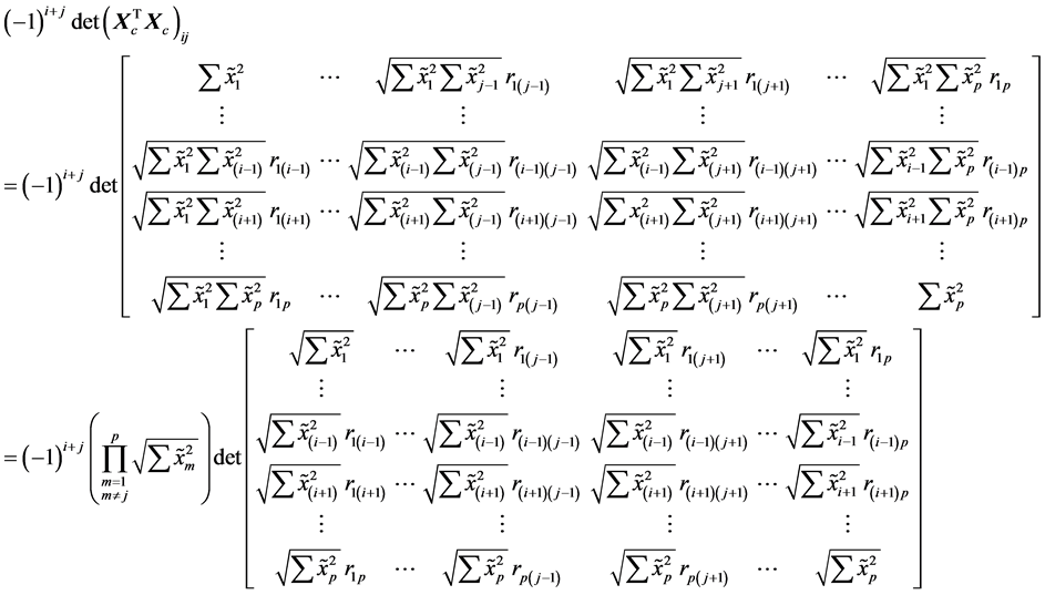
   In many applications, such as in multivariate meta-analysis or in the construction of multivariate models from summary statistics, the covariance of regression coefficients needs to be calculated without having access to individual patients’ data. In this work, we derive an alternative analytic expression for the covariance matrix of the regression coefficients in a multiple linear regression model. In contrast to the well-known expressions which make use of the cross-product matrix and hence require access to individual data, we express the covariance matrix of the regression coefficients directly in terms of covariance matrix of the explanatory variables. In particular, we show that the covariance matrix of the regression coefficients can be calculated using the matrix of the partial correlation coefficients of the explanatory variables, which in turn can be calculated easily from the correlation matrix of the explanatory variables. This is very important since the covariance matrix of the explanatory variables can be easily obtained or imputed using data from the literature, without requiring access to individual data. Two important applications of the method are discussed, namely the multivariate meta-analysis of regression coefficients and the so-called synthesis analysis, and the aim of which is to combine in a single predictive model, information from different variables. The estimator proposed in this work can increase the usefulness of these methods providing better results, as seen by application in a publicly available dataset. Source code is provided in the Appendix and in http://www.compgen.org/tools/regression.  
    
 
</p></abstract><kwd-group><kwd>Meta-Analysis</kwd><kwd> Linear Regression</kwd><kwd> Covariance Matrix</kwd><kwd> Regression Coefficients</kwd><kwd> Synthesis Analysis</kwd></kwd-group></article-meta></front><body><sec id="s1"><title>1. Introduction</title><p>The linear regression model is one of the oldest and most commonly used models in the statistical literature and it is widely used in a variety of disciplines ranging from medicine and genetics to econometrics, marketing, social sciences and psychology. Moreover, the relations of the linear regression model to other commonly used methods such as the t-test, the Analysis of Variance (ANOVA) and the Analysis of Covariance (ANCOVA) [<xref ref-type="bibr" rid="scirp.61997-ref1">1</xref>] [<xref ref-type="bibr" rid="scirp.61997-ref2">2</xref>] , as well as the role played by the multivariate normal distribution in multivariate statistics, place the linear model in the centre of interest in many fields of statistics.</p><p>In several applications, expressions for estimates of various parameters of the multiple regression models in terms of the summary statistics are needed. This is more evident in the general area of research synthesis methods, in which a researcher seeks to combine multiple sources of evidence across studies. For instance, in meta- analysis of regression coefficients [<xref ref-type="bibr" rid="scirp.61997-ref3">3</xref>] , which is a special case of multivariate meta-analysis [<xref ref-type="bibr" rid="scirp.61997-ref4">4</xref>] [<xref ref-type="bibr" rid="scirp.61997-ref5">5</xref>] , one is interested in the covariance matrix of the coefficients obtained in various studies, in order to perform a multivariate meta-analysis that takes properly into account the correlations among the estimates. The synthesis of regression coefficients has received increased attention in recent years [<xref ref-type="bibr" rid="scirp.61997-ref3">3</xref>] . This growing interest is probably related to the increasing complexity of the models investigated in primary research, and this seems to be the case for both biological [<xref ref-type="bibr" rid="scirp.61997-ref6">6</xref>] [<xref ref-type="bibr" rid="scirp.61997-ref7">7</xref>] as well as social sciences [<xref ref-type="bibr" rid="scirp.61997-ref8">8</xref>] -[<xref ref-type="bibr" rid="scirp.61997-ref11">11</xref>] . However, as Becker and Wu point out in their work: “the covariance matrix among the slopes in primary studies is rarely reported (though matrices of correlations among predictors are sometimes reported)” [<xref ref-type="bibr" rid="scirp.61997-ref3">3</xref>] . A well-known result from linear regression theory suggests that the covariance matrix of the coefficients depends on the cross-product matrix<inline-formula><inline-graphic xlink:href="http://html.scirp.org/file/5-1240581x7.png" xlink:type="simple"/></inline-formula>, where <inline-formula><inline-graphic xlink:href="http://html.scirp.org/file/5-1240581x8.png" xlink:type="simple"/></inline-formula> is the design matrix of the independent variables. Thus, in such a case, one needs to have access to individual data, something which is difficult and time-consuming.</p><p>Another example is the case of the so-called “synthesis analysis”, the aim of which is to combine in a single predictive model information from different variables. Synthesis analysis differs from traditional meta-analysis, since we are not synthesizing similar outcomes across different studies, but instead, we are trying to construct a multivariate model from pairwise associations, or to update a previously created model using external information (i.e. for an additional variable). For example, let’s consider the case of a multiple linear regression model that</p><p>relates the de-pendent variable, y, with p independent variables<inline-formula><inline-graphic xlink:href="http://html.scirp.org/file/5-1240581x9.png" xlink:type="simple"/></inline-formula>. The aim of the method is to build</p><p>the multivariate model that relates all predictors, however, not the individual data, but rather the information arising from the pairwise relationships among the variables. Samsa and coworkers were the first to provide details of such method. They used the univariate linear regressions of each x<sub>i</sub> against y and the correlation matrix that describes the linear relationships among the x<sub>i</sub>’s [<xref ref-type="bibr" rid="scirp.61997-ref12">12</xref>] . However, they did not provide an estimate for the covariance matrix. Later, Zhou and coworkers presented a different version of the method in which they used the univariate linear regressions of each x<sub>i</sub> against y along with the simple regressions that related each pair of x<sub>i</sub>’s [<xref ref-type="bibr" rid="scirp.61997-ref13">13</xref>] . Their method was based on solving a linear system of equations and they also described a method for calculating the variance-covariance matrix of the estimated coefficients using the multivariate delta method, utilizing the estimated variance-covariance matrix of the individual regression models. Such methods could be very important for instance for adjusting a previously obtained estimate for a potential confounder, for adjusting the results of a new analysis using estimates from the literature [<xref ref-type="bibr" rid="scirp.61997-ref14">14</xref>] , or for constructing and updating multivariate risk models [<xref ref-type="bibr" rid="scirp.61997-ref15">15</xref>] -[<xref ref-type="bibr" rid="scirp.61997-ref17">17</xref>] .</p><p>In this work, we derive an analytic expression for the covariance matrix of the regression coefficients in a multiple linear regression model. In contrast to the well-known expressions which make use of the cross-product matrix<inline-formula><inline-graphic xlink:href="http://html.scirp.org/file/5-1240581x10.png" xlink:type="simple"/></inline-formula>, we express the covariance matrix of the regression coefficients directly in terms of covariance matrix of the explanatory variables. This is very important since the covariance matrix of the explanatory variables can be easily obtained, or even imputed using data from the literature, without requiring access to individual data. In the following, in the Methods section we first present the details of synthesis analysis (2.1) and meta-analysis (2.2), in order to establish notation. Then, in Section (2.3) we present the classical framework of the multivariate normal model on which the problem is based and we give some results concerning some previously published estimators. Afterwards, in Section (2.4) we present the main result consisting of the analytical expression for the covariance of the regression coefficients. Finally, in Section (3) the method is applied to a real dataset, both in a meta-analysis and a synthesis analysis framework. Source code that implements the method, as well as the derivations of the main results are given in Appendix.</p></sec><sec id="s2"><title>2. Methods</title><sec id="s2_1"><title>2.1. Synthesis Analysis</title><p>The aim of synthesis analysis is to combine in a single predictive model, information from different variables. For instance, consider the case of a multiple linear regression model that relates the dependent variable, y, with p</p><p>independent variables,<inline-formula><inline-graphic xlink:href="http://html.scirp.org/file/5-1240581x11.png" xlink:type="simple"/></inline-formula>. The traditional linear regression, models the expectation of y given<inline-formula><inline-graphic xlink:href="http://html.scirp.org/file/5-1240581x12.png" xlink:type="simple"/></inline-formula>. as a linear combination of the covariates:</p><disp-formula id="scirp.61997-formula96"><label>(1)</label><graphic position="anchor" xlink:href="http://html.scirp.org/file/5-1240581x13.png"  xlink:type="simple"/></disp-formula><p>The aim of the method is to build the model in Equation (1), in other words, to find the estimates of the pa-</p><p>rameters<inline-formula><inline-graphic xlink:href="http://html.scirp.org/file/5-1240581x14.png" xlink:type="simple"/></inline-formula>, using however not the individual data, but rather the information arising from the pair-</p><p>wise relationships among the variables. In the following, the regression coefficients are the elements of the (p +</p><p>1) &#215; 1 matrix<inline-formula><inline-graphic xlink:href="http://html.scirp.org/file/5-1240581x15.png" xlink:type="simple"/></inline-formula>, where<inline-formula><inline-graphic xlink:href="http://html.scirp.org/file/5-1240581x16.png" xlink:type="simple"/></inline-formula>. These relationships could be, from the one hand the univariate linear regressions of each x<sub>i</sub> against y:</p><disp-formula id="scirp.61997-formula97"><label>(2)</label><graphic position="anchor" xlink:href="http://html.scirp.org/file/5-1240581x17.png"  xlink:type="simple"/></disp-formula><p>On the other hand, we could either have the simple regressions that relate each pair of x<sub>i</sub>’s:</p><disp-formula id="scirp.61997-formula98"><label>(3)</label><graphic position="anchor" xlink:href="http://html.scirp.org/file/5-1240581x18.png"  xlink:type="simple"/></disp-formula><p>or, the correlation matrix that describes the linear relationships among the x<sub>i</sub>’s:</p><disp-formula id="scirp.61997-formula99"><label>(4)</label><graphic position="anchor" xlink:href="http://html.scirp.org/file/5-1240581x19.png"  xlink:type="simple"/></disp-formula><p>In Equation (4), the Pearson’s correlation coefficient between x<sub>i</sub> and x<sub>j</sub> are denoted by r<sub>ij</sub> for 1 ≤ i, j ≤ p. The first approach for synthesis analysis was presented by Samsa and coworkers [<xref ref-type="bibr" rid="scirp.61997-ref12">12</xref>] who used Equation (2) and Equation (3) in order to calculate the estimates of Equation (1). In particular, the authors used a previously known result that relates <inline-formula><inline-graphic xlink:href="http://html.scirp.org/file/5-1240581x20.png" xlink:type="simple"/></inline-formula> to the matrices A, S, where <inline-formula><inline-graphic xlink:href="http://html.scirp.org/file/5-1240581x21.png" xlink:type="simple"/></inline-formula> is the p &#215; 1 matrix of the regression coefficients</p><p><inline-formula><inline-graphic xlink:href="http://html.scirp.org/file/5-1240581x22.png" xlink:type="simple"/></inline-formula>from the multivariate model of Equation (1), A is the p &#215; 1 matrix of the regression coefficients of</p><p>Equation (2), S is the p &#215; 1 matrix of the standard deviations of the x<sub>i</sub> covariates and R<sub>x</sub> is given by Equation (4). If we denote A and S by:</p><disp-formula id="scirp.61997-formula100"><label>(5)</label><graphic position="anchor" xlink:href="http://html.scirp.org/file/5-1240581x23.png"  xlink:type="simple"/></disp-formula><p>then the regression coefficients can be calculated by:</p><disp-formula id="scirp.61997-formula101"><label>(6)</label><graphic position="anchor" xlink:href="http://html.scirp.org/file/5-1240581x24.png"  xlink:type="simple"/></disp-formula><p>In Equation (6), <inline-formula><inline-graphic xlink:href="http://html.scirp.org/file/5-1240581x25.png" xlink:type="simple"/></inline-formula>stands for the element-wise multiplication (also known as the Hadamard product or dot matrix product) and similarly the division (/) is also element-wise. This method, provides estimates for the re-</p><p>gression coefficient<inline-formula><inline-graphic xlink:href="http://html.scirp.org/file/5-1240581x26.png" xlink:type="simple"/></inline-formula>, and in order for the intercept, β<sub>0</sub>, to be calculated, one would need to use the estimated <inline-formula><inline-graphic xlink:href="http://html.scirp.org/file/5-1240581x26.png" xlink:type="simple"/></inline-formula><inline-formula><inline-graphic xlink:href="http://html.scirp.org/file/5-1240581x27.png" xlink:type="simple"/></inline-formula> along with the mean values of the variables. Finally, we should mention that the method</p><p>as described did not provide an estimate for the variance of the coefficients. Thus, construction of confidence intervals and assessment of the statistical significance of the covariates could not be carried out. In a latter work, Zhou and coworkers [<xref ref-type="bibr" rid="scirp.61997-ref13">13</xref>] developed a different method. First, they took expectations on both sides of Equation (1) conditioning on x<sub>i</sub>:</p><disp-formula id="scirp.61997-formula102"><label>(7)</label><graphic position="anchor" xlink:href="http://html.scirp.org/file/5-1240581x28.png"  xlink:type="simple"/></disp-formula><p>Then, by combining Equation (2), Equation (3) and Equation (7), they obtained the following result:</p><disp-formula id="scirp.61997-formula103"><label>(8)</label><graphic position="anchor" xlink:href="http://html.scirp.org/file/5-1240581x29.png"  xlink:type="simple"/></disp-formula><p>Using now Equation (8), they obtained a system of p equations for the p unknown parameters, which are the p elements of<inline-formula><inline-graphic xlink:href="http://html.scirp.org/file/5-1240581x30.png" xlink:type="simple"/></inline-formula>, <inline-formula><inline-graphic xlink:href="http://html.scirp.org/file/5-1240581x30.png" xlink:type="simple"/></inline-formula><inline-formula><inline-graphic xlink:href="http://html.scirp.org/file/5-1240581x31.png" xlink:type="simple"/></inline-formula>, that can be easily solved and p equations for the intercept β<sub>0</sub>, which however</p><p>they proved that lead to a unique solution. The authors described also a method for calculating the variance-covariance matrix of the estimated coefficients using the multivariate delta method, utilizing the estimated variance-covariance matrix of the individual regression models (Equation (2) and Equation (3)).</p><p>The method is very interesting in that it does not assume normality of the covariates in order to estimate the parameters and thus it is expected to be more robust in case of non-normally distributed variables (but assumes the normality of the estimated parameters in order to use the delta method). On the other hand, the method is quite difficult to be implemented for an arbitrary number of covariates. The system of equations arising from Equation (8) should be solved explicitly and the solution will be more difficult as the number of covariates increases (the authors provided explicit solutions for p = 2 and p = 3). The major difficulty however, lies in the calculation of the covariance matrix with the delta method. The difficulty is particularly evident if we consider that the β<sub>i</sub>’s are highly non-linear functions of the α<sub>i</sub>’s and γ<sub>i</sub>’s and thus the partial derivatives require explicit calculations, which are different for different p and can be done only using software that perform symbolic calculations.</p></sec><sec id="s2_2"><title>2.2. Meta-Analysis of Regression Coefficients</title><p>In the meta-analysis of regression coefficients, the problem is different. Here, we have a set <inline-formula><inline-graphic xlink:href="http://html.scirp.org/file/5-1240581x32.png" xlink:type="simple"/></inline-formula> of</p><p>p regression coefficients arising from k studies (<inline-formula><inline-graphic xlink:href="http://html.scirp.org/file/5-1240581x33.png" xlink:type="simple"/></inline-formula>) and we want to combine them in order to obtain the overall mean<inline-formula><inline-graphic xlink:href="http://html.scirp.org/file/5-1240581x33.png" xlink:type="simple"/></inline-formula><inline-formula><inline-graphic xlink:href="http://html.scirp.org/file/5-1240581x34.png" xlink:type="simple"/></inline-formula>. Thus, it is a special case of multivariate random-effects meta-analysis [<xref ref-type="bibr" rid="scirp.61997-ref4">4</xref>] [<xref ref-type="bibr" rid="scirp.61997-ref5">5</xref>] ; we denote</p><p><inline-formula><inline-graphic xlink:href="http://html.scirp.org/file/5-1240581x35.png" xlink:type="simple"/></inline-formula>and usually assume that <inline-formula><inline-graphic xlink:href="http://html.scirp.org/file/5-1240581x35.png" xlink:type="simple"/></inline-formula><inline-formula><inline-graphic xlink:href="http://html.scirp.org/file/5-1240581x36.png" xlink:type="simple"/></inline-formula> is distributed following a multivariate normal distribution around the true means<inline-formula><inline-graphic xlink:href="http://html.scirp.org/file/5-1240581x35.png" xlink:type="simple"/></inline-formula><inline-formula><inline-graphic xlink:href="http://html.scirp.org/file/5-1240581x36.png" xlink:type="simple"/></inline-formula><inline-formula><inline-graphic xlink:href="http://html.scirp.org/file/5-1240581x37.png" xlink:type="simple"/></inline-formula>, according to the marginal model:</p><disp-formula id="scirp.61997-formula104"><label>(9)</label><graphic position="anchor" xlink:href="http://html.scirp.org/file/5-1240581x38.png"  xlink:type="simple"/></disp-formula><p>In the above model, we denote by <inline-formula><inline-graphic xlink:href="http://html.scirp.org/file/5-1240581x39.png" xlink:type="simple"/></inline-formula> the within-studies covariance matrix:</p><disp-formula id="scirp.61997-formula105"><label>(10)</label><graphic position="anchor" xlink:href="http://html.scirp.org/file/5-1240581x40.png"  xlink:type="simple"/></disp-formula><p>and by Ω the between-studies covariance matrix, given by:</p><disp-formula id="scirp.61997-formula106"><label>(11)</label><graphic position="anchor" xlink:href="http://html.scirp.org/file/5-1240581x41.png"  xlink:type="simple"/></disp-formula><p>This is the classic model of multivariate meta-analysis used in several applications [<xref ref-type="bibr" rid="scirp.61997-ref4">4</xref>] [<xref ref-type="bibr" rid="scirp.61997-ref5">5</xref>] [<xref ref-type="bibr" rid="scirp.61997-ref18">18</xref>] . For fitting this model, there are several alternatives, such as Maximum Likelihood (ML), Restricted Maximum Likelihood (REML) or the multivariate method of moments (MM), all of which however require that the diagonal elements of C<sub>s</sub>. These are the study-specific estimates of the variance that are assumed known, whereas the off-diagonal elements correspond to the pairwise within-studies covariances, thus for <inline-formula><inline-graphic xlink:href="http://html.scirp.org/file/5-1240581x42.png" xlink:type="simple"/></inline-formula> we have:</p><disp-formula id="scirp.61997-formula107"><label>(12)</label><graphic position="anchor" xlink:href="http://html.scirp.org/file/5-1240581x43.png"  xlink:type="simple"/></disp-formula><p>On the other hand, the between studies covariance matrix is estimated from the data. Of course, in model of Equation (9) we could also use <inline-formula><inline-graphic xlink:href="http://html.scirp.org/file/5-1240581x44.png" xlink:type="simple"/></inline-formula> and include the intercept as well. However, this will rarely be needed in practical applications where the interest lies in the estimation of covariate effects.</p><p>The major problem in this method, is, as Becker and Wu point out that “in practice, the covariance matrix among the slopes in primary studies is rarely reported (though matrices of correlations among predictors are sometimes reported)” [<xref ref-type="bibr" rid="scirp.61997-ref3">3</xref>] . Usually, ignoring or approximating the within studies covariance matrix produce reliable estimates for the fixed effects parameters but biased estimates for the variance [<xref ref-type="bibr" rid="scirp.61997-ref19">19</xref>] [<xref ref-type="bibr" rid="scirp.61997-ref20">20</xref>] . Thus, ideally one would want to include reliable estimates for the within studies covariances in order to gain the maximum from the multivariate meta-analysis. Currently, since the majority of studies do not report the covariance matrices, a literature-based (i.e. without having access to individual data) meta-analysis would be forced to assume zero correlations between the regression coefficients, limiting this way the efficiency of the method. An alternative, would be to use the model of Riley and coworkers, which, being no-hierarchical, maintains the individual weighting of each study in the analysis but includes only one overall correlation parameter, removing this way the need to know the within-study correlations [<xref ref-type="bibr" rid="scirp.61997-ref21">21</xref>] . For other effect sizes, such as the odds ratio, the relative risk and so on, recent studies have shown that under certain conditions, the correlation can be estimated using only the pairwise correlations of the variables involved [<xref ref-type="bibr" rid="scirp.61997-ref22">22</xref>] [<xref ref-type="bibr" rid="scirp.61997-ref23">23</xref>] . Thus, a similar approach can be followed here concerning the regression coefficients.</p></sec><sec id="s2_3"><title>2.3. The General Method</title><p>We will begin with the multivariate normal model. This is one of the two main approaches for formulating a regression problem (the other one is the approach that assumes that the independent variables are fixed by design). Even though the two approaches are conceptually very different, it is well known that concerning the estimation of the regression parameters (coefficients and their variance), they yield exactly the same results. Consider we</p><p>have p + 1 variables, y and <inline-formula><inline-graphic xlink:href="http://html.scirp.org/file/5-1240581x45.png" xlink:type="simple"/></inline-formula> that are distributed according to a multivariate normal distribution. The traditional linear regression, models the expectation of y given <inline-formula><inline-graphic xlink:href="http://html.scirp.org/file/5-1240581x45.png" xlink:type="simple"/></inline-formula><inline-formula><inline-graphic xlink:href="http://html.scirp.org/file/5-1240581x46.png" xlink:type="simple"/></inline-formula> as a linear combination of the covariates <inline-formula><inline-graphic xlink:href="http://html.scirp.org/file/5-1240581x45.png" xlink:type="simple"/></inline-formula><inline-formula><inline-graphic xlink:href="http://html.scirp.org/file/5-1240581x46.png" xlink:type="simple"/></inline-formula><inline-formula><inline-graphic xlink:href="http://html.scirp.org/file/5-1240581x47.png" xlink:type="simple"/></inline-formula> according to Equation (1). If we denote by<inline-formula><inline-graphic xlink:href="http://html.scirp.org/file/5-1240581x45.png" xlink:type="simple"/></inline-formula><inline-formula><inline-graphic xlink:href="http://html.scirp.org/file/5-1240581x46.png" xlink:type="simple"/></inline-formula><inline-formula><inline-graphic xlink:href="http://html.scirp.org/file/5-1240581x47.png" xlink:type="simple"/></inline-formula><inline-formula><inline-graphic xlink:href="http://html.scirp.org/file/5-1240581x48.png" xlink:type="simple"/></inline-formula>, <inline-formula><inline-graphic xlink:href="http://html.scirp.org/file/5-1240581x45.png" xlink:type="simple"/></inline-formula><inline-formula><inline-graphic xlink:href="http://html.scirp.org/file/5-1240581x46.png" xlink:type="simple"/></inline-formula><inline-formula><inline-graphic xlink:href="http://html.scirp.org/file/5-1240581x47.png" xlink:type="simple"/></inline-formula><inline-formula><inline-graphic xlink:href="http://html.scirp.org/file/5-1240581x48.png" xlink:type="simple"/></inline-formula><inline-formula><inline-graphic xlink:href="http://html.scirp.org/file/5-1240581x49.png" xlink:type="simple"/></inline-formula>and by Σ the <inline-formula><inline-graphic xlink:href="http://html.scirp.org/file/5-1240581x45.png" xlink:type="simple"/></inline-formula><inline-formula><inline-graphic xlink:href="http://html.scirp.org/file/5-1240581x46.png" xlink:type="simple"/></inline-formula><inline-formula><inline-graphic xlink:href="http://html.scirp.org/file/5-1240581x47.png" xlink:type="simple"/></inline-formula><inline-formula><inline-graphic xlink:href="http://html.scirp.org/file/5-1240581x48.png" xlink:type="simple"/></inline-formula><inline-formula><inline-graphic xlink:href="http://html.scirp.org/file/5-1240581x49.png" xlink:type="simple"/></inline-formula><inline-formula><inline-graphic xlink:href="http://html.scirp.org/file/5-1240581x50.png" xlink:type="simple"/></inline-formula> variance-covariance matrix:</p><disp-formula id="scirp.61997-formula108"><label>(13)</label><graphic position="anchor" xlink:href="http://html.scirp.org/file/5-1240581x51.png"  xlink:type="simple"/></disp-formula><p>then we will have <inline-formula><inline-graphic xlink:href="http://html.scirp.org/file/5-1240581x52.png" xlink:type="simple"/></inline-formula> and a well-known result from multivariate statistics allows the arbitrary partitioning of Σ in order to obtain:</p><disp-formula id="scirp.61997-formula109"><label>(14)</label><graphic position="anchor" xlink:href="http://html.scirp.org/file/5-1240581x53.png"  xlink:type="simple"/></disp-formula><p>In this case, the partial vectors are once again multivariate normal with<inline-formula><inline-graphic xlink:href="http://html.scirp.org/file/5-1240581x54.png" xlink:type="simple"/></inline-formula>, <inline-formula><inline-graphic xlink:href="http://html.scirp.org/file/5-1240581x54.png" xlink:type="simple"/></inline-formula><inline-formula><inline-graphic xlink:href="http://html.scirp.org/file/5-1240581x55.png" xlink:type="simple"/></inline-formula> with Σ<sub>11</sub>, Σ<sub>12</sub>, Σ<sub>21</sub>, and Σ<sub>22</sub> being the partial covariance matrices. Then, the conditional distribution of Y<sub>1</sub> given Y<sub>2</sub> (i.e. the regression of Y<sub>2</sub> on Y<sub>1</sub>) is given by:</p><disp-formula id="scirp.61997-formula110"><label>(15)</label><graphic position="anchor" xlink:href="http://html.scirp.org/file/5-1240581x56.png"  xlink:type="simple"/></disp-formula><p>If we partition Σ in order to obtain Equation (1), then the partial covariance matrices would be:</p><disp-formula id="scirp.61997-formula111"><label>(16)</label><graphic position="anchor" xlink:href="http://html.scirp.org/file/5-1240581x57.png"  xlink:type="simple"/></disp-formula><p>whereas, Y<sub>1</sub> would be a univariate normal<inline-formula><inline-graphic xlink:href="http://html.scirp.org/file/5-1240581x58.png" xlink:type="simple"/></inline-formula>. Then, the regression coefficients of Equation (1), with the exception of the intercept, will be given by:</p><disp-formula id="scirp.61997-formula112"><label>(17)</label><graphic position="anchor" xlink:href="http://html.scirp.org/file/5-1240581x59.png"  xlink:type="simple"/></disp-formula><p>The intercept is given simply as a function of the p regression coefficients and the mean vectors of y and x<sub>i</sub>’s:</p><disp-formula id="scirp.61997-formula113"><graphic  xlink:href="http://html.scirp.org/file/5-1240581x60.png"  xlink:type="simple"/></disp-formula><p>The covariance matrix of the coefficients in Equation (1) including the intercept is given by:</p><disp-formula id="scirp.61997-formula114"><label>(18)</label><graphic position="anchor" xlink:href="http://html.scirp.org/file/5-1240581x61.png"  xlink:type="simple"/></disp-formula><p>where <inline-formula><inline-graphic xlink:href="http://html.scirp.org/file/5-1240581x62.png" xlink:type="simple"/></inline-formula> denotes the <inline-formula><inline-graphic xlink:href="http://html.scirp.org/file/5-1240581x62.png" xlink:type="simple"/></inline-formula><inline-formula><inline-graphic xlink:href="http://html.scirp.org/file/5-1240581x63.png" xlink:type="simple"/></inline-formula> design matrix of the independent variables, <inline-formula><inline-graphic xlink:href="http://html.scirp.org/file/5-1240581x62.png" xlink:type="simple"/></inline-formula><inline-formula><inline-graphic xlink:href="http://html.scirp.org/file/5-1240581x63.png" xlink:type="simple"/></inline-formula><inline-formula><inline-graphic xlink:href="http://html.scirp.org/file/5-1240581x64.png" xlink:type="simple"/></inline-formula>the transpose matrix of <inline-formula><inline-graphic xlink:href="http://html.scirp.org/file/5-1240581x62.png" xlink:type="simple"/></inline-formula><inline-formula><inline-graphic xlink:href="http://html.scirp.org/file/5-1240581x63.png" xlink:type="simple"/></inline-formula><inline-formula><inline-graphic xlink:href="http://html.scirp.org/file/5-1240581x64.png" xlink:type="simple"/></inline-formula><inline-formula><inline-graphic xlink:href="http://html.scirp.org/file/5-1240581x65.png" xlink:type="simple"/></inline-formula> and<inline-formula><inline-graphic xlink:href="http://html.scirp.org/file/5-1240581x62.png" xlink:type="simple"/></inline-formula><inline-formula><inline-graphic xlink:href="http://html.scirp.org/file/5-1240581x63.png" xlink:type="simple"/></inline-formula><inline-formula><inline-graphic xlink:href="http://html.scirp.org/file/5-1240581x64.png" xlink:type="simple"/></inline-formula><inline-formula><inline-graphic xlink:href="http://html.scirp.org/file/5-1240581x65.png" xlink:type="simple"/></inline-formula><inline-formula><inline-graphic xlink:href="http://html.scirp.org/file/5-1240581x66.png" xlink:type="simple"/></inline-formula>. Notice that<inline-formula><inline-graphic xlink:href="http://html.scirp.org/file/5-1240581x62.png" xlink:type="simple"/></inline-formula><inline-formula><inline-graphic xlink:href="http://html.scirp.org/file/5-1240581x63.png" xlink:type="simple"/></inline-formula><inline-formula><inline-graphic xlink:href="http://html.scirp.org/file/5-1240581x64.png" xlink:type="simple"/></inline-formula><inline-formula><inline-graphic xlink:href="http://html.scirp.org/file/5-1240581x65.png" xlink:type="simple"/></inline-formula><inline-formula><inline-graphic xlink:href="http://html.scirp.org/file/5-1240581x66.png" xlink:type="simple"/></inline-formula><inline-formula><inline-graphic xlink:href="http://html.scirp.org/file/5-1240581x67.png" xlink:type="simple"/></inline-formula>, since <inline-formula><inline-graphic xlink:href="http://html.scirp.org/file/5-1240581x62.png" xlink:type="simple"/></inline-formula><inline-formula><inline-graphic xlink:href="http://html.scirp.org/file/5-1240581x63.png" xlink:type="simple"/></inline-formula><inline-formula><inline-graphic xlink:href="http://html.scirp.org/file/5-1240581x64.png" xlink:type="simple"/></inline-formula><inline-formula><inline-graphic xlink:href="http://html.scirp.org/file/5-1240581x65.png" xlink:type="simple"/></inline-formula><inline-formula><inline-graphic xlink:href="http://html.scirp.org/file/5-1240581x66.png" xlink:type="simple"/></inline-formula><inline-formula><inline-graphic xlink:href="http://html.scirp.org/file/5-1240581x67.png" xlink:type="simple"/></inline-formula><inline-formula><inline-graphic xlink:href="http://html.scirp.org/file/5-1240581x68.png" xlink:type="simple"/></inline-formula> is a symmetric matrix and <inline-formula><inline-graphic xlink:href="http://html.scirp.org/file/5-1240581x62.png" xlink:type="simple"/></inline-formula><inline-formula><inline-graphic xlink:href="http://html.scirp.org/file/5-1240581x63.png" xlink:type="simple"/></inline-formula><inline-formula><inline-graphic xlink:href="http://html.scirp.org/file/5-1240581x64.png" xlink:type="simple"/></inline-formula><inline-formula><inline-graphic xlink:href="http://html.scirp.org/file/5-1240581x65.png" xlink:type="simple"/></inline-formula><inline-formula><inline-graphic xlink:href="http://html.scirp.org/file/5-1240581x66.png" xlink:type="simple"/></inline-formula><inline-formula><inline-graphic xlink:href="http://html.scirp.org/file/5-1240581x67.png" xlink:type="simple"/></inline-formula><inline-formula><inline-graphic xlink:href="http://html.scirp.org/file/5-1240581x68.png" xlink:type="simple"/></inline-formula><inline-formula><inline-graphic xlink:href="http://html.scirp.org/file/5-1240581x69.png" xlink:type="simple"/></inline-formula>. An alternative estimate for <inline-formula><inline-graphic xlink:href="http://html.scirp.org/file/5-1240581x62.png" xlink:type="simple"/></inline-formula><inline-formula><inline-graphic xlink:href="http://html.scirp.org/file/5-1240581x63.png" xlink:type="simple"/></inline-formula><inline-formula><inline-graphic xlink:href="http://html.scirp.org/file/5-1240581x64.png" xlink:type="simple"/></inline-formula><inline-formula><inline-graphic xlink:href="http://html.scirp.org/file/5-1240581x65.png" xlink:type="simple"/></inline-formula><inline-formula><inline-graphic xlink:href="http://html.scirp.org/file/5-1240581x66.png" xlink:type="simple"/></inline-formula><inline-formula><inline-graphic xlink:href="http://html.scirp.org/file/5-1240581x67.png" xlink:type="simple"/></inline-formula><inline-formula><inline-graphic xlink:href="http://html.scirp.org/file/5-1240581x68.png" xlink:type="simple"/></inline-formula><inline-formula><inline-graphic xlink:href="http://html.scirp.org/file/5-1240581x69.png" xlink:type="simple"/></inline-formula><inline-formula><inline-graphic xlink:href="http://html.scirp.org/file/5-1240581x70.png" xlink:type="simple"/></inline-formula> in terms of the centralised design matrix<inline-formula><inline-graphic xlink:href="http://html.scirp.org/file/5-1240581x62.png" xlink:type="simple"/></inline-formula><inline-formula><inline-graphic xlink:href="http://html.scirp.org/file/5-1240581x63.png" xlink:type="simple"/></inline-formula><inline-formula><inline-graphic xlink:href="http://html.scirp.org/file/5-1240581x64.png" xlink:type="simple"/></inline-formula><inline-formula><inline-graphic xlink:href="http://html.scirp.org/file/5-1240581x65.png" xlink:type="simple"/></inline-formula><inline-formula><inline-graphic xlink:href="http://html.scirp.org/file/5-1240581x66.png" xlink:type="simple"/></inline-formula><inline-formula><inline-graphic xlink:href="http://html.scirp.org/file/5-1240581x67.png" xlink:type="simple"/></inline-formula><inline-formula><inline-graphic xlink:href="http://html.scirp.org/file/5-1240581x68.png" xlink:type="simple"/></inline-formula><inline-formula><inline-graphic xlink:href="http://html.scirp.org/file/5-1240581x69.png" xlink:type="simple"/></inline-formula><inline-formula><inline-graphic xlink:href="http://html.scirp.org/file/5-1240581x70.png" xlink:type="simple"/></inline-formula><inline-formula><inline-graphic xlink:href="http://html.scirp.org/file/5-1240581x71.png" xlink:type="simple"/></inline-formula>, is discussed in Appendix C.</p><p>In Appendix A, we show that the estimated regression coefficients by this method are identical to the ones obtained by Samsa and coworkers [<xref ref-type="bibr" rid="scirp.61997-ref12">12</xref>] . In other words, we show that:</p><disp-formula id="scirp.61997-formula115"><label>(19)</label><graphic position="anchor" xlink:href="http://html.scirp.org/file/5-1240581x72.png"  xlink:type="simple"/></disp-formula><p>It is obvious that the estimate proposed by Samsa and coworkers [<xref ref-type="bibr" rid="scirp.61997-ref12">12</xref>] is just a re-parameterization of a well-known result and produces identical estimates.</p><p>Another commonly used formula, can be derive the estimation of the standardised regression coefficients<inline-formula><inline-graphic xlink:href="http://html.scirp.org/file/5-1240581x73.png" xlink:type="simple"/></inline-formula>, for each<inline-formula><inline-graphic xlink:href="http://html.scirp.org/file/5-1240581x73.png" xlink:type="simple"/></inline-formula><inline-formula><inline-graphic xlink:href="http://html.scirp.org/file/5-1240581x74.png" xlink:type="simple"/></inline-formula>, using the correlation matrices <inline-formula><inline-graphic xlink:href="http://html.scirp.org/file/5-1240581x73.png" xlink:type="simple"/></inline-formula><inline-formula><inline-graphic xlink:href="http://html.scirp.org/file/5-1240581x74.png" xlink:type="simple"/></inline-formula><inline-formula><inline-graphic xlink:href="http://html.scirp.org/file/5-1240581x75.png" xlink:type="simple"/></inline-formula> of Equation (4) and</p><p><inline-formula><inline-graphic xlink:href="http://html.scirp.org/file/5-1240581x76.png" xlink:type="simple"/></inline-formula>, where <inline-formula><inline-graphic xlink:href="http://html.scirp.org/file/5-1240581x76.png" xlink:type="simple"/></inline-formula><inline-formula><inline-graphic xlink:href="http://html.scirp.org/file/5-1240581x77.png" xlink:type="simple"/></inline-formula> are the Pearson’s correlation coefficient between <inline-formula><inline-graphic xlink:href="http://html.scirp.org/file/5-1240581x76.png" xlink:type="simple"/></inline-formula><inline-formula><inline-graphic xlink:href="http://html.scirp.org/file/5-1240581x77.png" xlink:type="simple"/></inline-formula><inline-formula><inline-graphic xlink:href="http://html.scirp.org/file/5-1240581x78.png" xlink:type="simple"/></inline-formula> and y. Then, the matrix <inline-formula><inline-graphic xlink:href="http://html.scirp.org/file/5-1240581x76.png" xlink:type="simple"/></inline-formula><inline-formula><inline-graphic xlink:href="http://html.scirp.org/file/5-1240581x77.png" xlink:type="simple"/></inline-formula><inline-formula><inline-graphic xlink:href="http://html.scirp.org/file/5-1240581x78.png" xlink:type="simple"/></inline-formula><inline-formula><inline-graphic xlink:href="http://html.scirp.org/file/5-1240581x79.png" xlink:type="simple"/></inline-formula> of standardised regression coefficients can be obtained by:</p><disp-formula id="scirp.61997-formula116"><label>(20)</label><graphic position="anchor" xlink:href="http://html.scirp.org/file/5-1240581x80.png"  xlink:type="simple"/></disp-formula><p>The standardised regression coefficients <inline-formula><inline-graphic xlink:href="http://html.scirp.org/file/5-1240581x81.png" xlink:type="simple"/></inline-formula> can be transformed to unstandardised regression coefficients <inline-formula><inline-graphic xlink:href="http://html.scirp.org/file/5-1240581x81.png" xlink:type="simple"/></inline-formula><inline-formula><inline-graphic xlink:href="http://html.scirp.org/file/5-1240581x82.png" xlink:type="simple"/></inline-formula> using<inline-formula><inline-graphic xlink:href="http://html.scirp.org/file/5-1240581x81.png" xlink:type="simple"/></inline-formula><inline-formula><inline-graphic xlink:href="http://html.scirp.org/file/5-1240581x82.png" xlink:type="simple"/></inline-formula><inline-formula><inline-graphic xlink:href="http://html.scirp.org/file/5-1240581x83.png" xlink:type="simple"/></inline-formula>, or in matrix form</p><disp-formula id="scirp.61997-formula117"><label>(21)</label><graphic position="anchor" xlink:href="http://html.scirp.org/file/5-1240581x84.png"  xlink:type="simple"/></disp-formula><p>where <inline-formula><inline-graphic xlink:href="http://html.scirp.org/file/5-1240581x85.png" xlink:type="simple"/></inline-formula> denotes the <inline-formula><inline-graphic xlink:href="http://html.scirp.org/file/5-1240581x85.png" xlink:type="simple"/></inline-formula><inline-formula><inline-graphic xlink:href="http://html.scirp.org/file/5-1240581x86.png" xlink:type="simple"/></inline-formula> diagonal matrix such that<inline-formula><inline-graphic xlink:href="http://html.scirp.org/file/5-1240581x85.png" xlink:type="simple"/></inline-formula><inline-formula><inline-graphic xlink:href="http://html.scirp.org/file/5-1240581x86.png" xlink:type="simple"/></inline-formula><inline-formula><inline-graphic xlink:href="http://html.scirp.org/file/5-1240581x87.png" xlink:type="simple"/></inline-formula>. In Appendix B, we show</p><p>that the coefficients obtained with Equation (20) and Equation (21), are identical to the ones obtained with the use of Equation (6) and Equation (17). That is, we show that:</p><disp-formula id="scirp.61997-formula118"><label>(22)</label><graphic position="anchor" xlink:href="http://html.scirp.org/file/5-1240581x88.png"  xlink:type="simple"/></disp-formula><p>Thus, it is clear that the three methods described above are equivalent and yield identical estimates</p><disp-formula id="scirp.61997-formula119"><label>(23)</label><graphic position="anchor" xlink:href="http://html.scirp.org/file/5-1240581x89.png"  xlink:type="simple"/></disp-formula></sec><sec id="s2_4"><title>2.4. Variance-Covariance Matrix</title><p>If we want to obtain the variance of the estimated coefficients, we need to turn to Equation (18), which requires explicit knowledge of the <inline-formula><inline-graphic xlink:href="http://html.scirp.org/file/5-1240581x90.png" xlink:type="simple"/></inline-formula> design matrix <inline-formula><inline-graphic xlink:href="http://html.scirp.org/file/5-1240581x90.png" xlink:type="simple"/></inline-formula><inline-formula><inline-graphic xlink:href="http://html.scirp.org/file/5-1240581x91.png" xlink:type="simple"/></inline-formula> and the cross-product matrix:</p><disp-formula id="scirp.61997-formula120"><label>(24)</label><graphic position="anchor" xlink:href="http://html.scirp.org/file/5-1240581x92.png"  xlink:type="simple"/></disp-formula><p>In synthesis analysis as well as in meta-analysis, one usually does not have access to n &#215; p individual data<inline-formula><inline-graphic xlink:href="http://html.scirp.org/file/5-1240581x93.png" xlink:type="simple"/></inline-formula>, and thus, we have to find a method to estimate the variance with information obtained from the published reports. As we already discussed, Samsa and coworkers [<xref ref-type="bibr" rid="scirp.61997-ref12">12</xref>] did not provide an estimate for the covariance matrix, whereas Zhou and coworkers [<xref ref-type="bibr" rid="scirp.61997-ref13">13</xref>] provided a difficult to obtain estimate, using the delta method. However, the variance of a regression coefficient (let’s say β<sub>i</sub>) can be obtained relatively easily from summary statistics and it can be shown to be equal to:</p><disp-formula id="scirp.61997-formula121"><label>(25)</label><graphic position="anchor" xlink:href="http://html.scirp.org/file/5-1240581x94.png"  xlink:type="simple"/></disp-formula><p>The formula in Equation (25) can be found in many textbooks with the proof traced back in earlier versions of Green’s Econometrics Analysis [<xref ref-type="bibr" rid="scirp.61997-ref24">24</xref>] ; another elegant proof can be found in [<xref ref-type="bibr" rid="scirp.61997-ref25">25</xref>] . Here, <inline-formula><inline-graphic xlink:href="http://html.scirp.org/file/5-1240581x95.png" xlink:type="simple"/></inline-formula>is the squared multiple correlation that relates x<sub>i</sub> with the rest of the independent variables, whereas σ<sup>2</sup> is the total variance of the</p><p>regression. The term <inline-formula><inline-graphic xlink:href="http://html.scirp.org/file/5-1240581x96.png" xlink:type="simple"/></inline-formula> is usually named “variance inflation factor”. In many applications, we may</p><p>conveniently assume that the total variance remains the same if we add x<sub>i </sub>in the model, so we may write the variance of the regression coefficient in the full model as a function of the variance of the coefficient in the univariate model of Equation (2):</p><disp-formula id="scirp.61997-formula122"><label>(26)</label><graphic position="anchor" xlink:href="http://html.scirp.org/file/5-1240581x97.png"  xlink:type="simple"/></disp-formula><p>Clearly, in most of the situations this is an upper bound [<xref ref-type="bibr" rid="scirp.61997-ref25">25</xref>] [<xref ref-type="bibr" rid="scirp.61997-ref26">26</xref>] that leads to conservative estimates but it may be useful in many practical applications. In order to evaluate Equation (25), we need to calculate <inline-formula><inline-graphic xlink:href="http://html.scirp.org/file/5-1240581x98.png" xlink:type="simple"/></inline-formula> and σ<sup>2</sup>. As we already said, σ<sup>2 </sup>can be obtained from:</p><disp-formula id="scirp.61997-formula123"><label>(27)</label><graphic position="anchor" xlink:href="http://html.scirp.org/file/5-1240581x99.png"  xlink:type="simple"/></disp-formula><p>We need to remind however, that since this quantity is usually estimated, in real applications we need to adjust it (see [<xref ref-type="bibr" rid="scirp.61997-ref27">27</xref>] pp 405) in order to obtain the unbiased estimator:</p><disp-formula id="scirp.61997-formula124"><label>(28)</label><graphic position="anchor" xlink:href="http://html.scirp.org/file/5-1240581x100.png"  xlink:type="simple"/></disp-formula><p>On the other hand, an easy way (among others) to obtain <inline-formula><inline-graphic xlink:href="http://html.scirp.org/file/5-1240581x101.png" xlink:type="simple"/></inline-formula> is using:</p><disp-formula id="scirp.61997-formula125"><label>(29)</label><graphic position="anchor" xlink:href="http://html.scirp.org/file/5-1240581x102.png"  xlink:type="simple"/></disp-formula><p>where υ<sub>ii</sub> is the i-th diagonal element of<inline-formula><inline-graphic xlink:href="http://html.scirp.org/file/5-1240581x103.png" xlink:type="simple"/></inline-formula>.</p><p>The main result of this work is to provide a closed-form expression for the covariance, that does not include<inline-formula><inline-graphic xlink:href="http://html.scirp.org/file/5-1240581x104.png" xlink:type="simple"/></inline-formula>. In Appendix C we show that the covariance is given by:</p><disp-formula id="scirp.61997-formula126"><label>(30)</label><graphic position="anchor" xlink:href="http://html.scirp.org/file/5-1240581x105.png"  xlink:type="simple"/></disp-formula><p>where <inline-formula><inline-graphic xlink:href="http://html.scirp.org/file/5-1240581x106.png" xlink:type="simple"/></inline-formula> is the ij-partial correlation of x<sub>i </sub>with x<sub>j</sub>-controlling for the remaining variables. For<inline-formula><inline-graphic xlink:href="http://html.scirp.org/file/5-1240581x106.png" xlink:type="simple"/></inline-formula><inline-formula><inline-graphic xlink:href="http://html.scirp.org/file/5-1240581x107.png" xlink:type="simple"/></inline-formula>, the ij-partial correlation coefficient is defined [<xref ref-type="bibr" rid="scirp.61997-ref28">28</xref>] as:</p><disp-formula id="scirp.61997-formula127"><label>(31)</label><graphic position="anchor" xlink:href="http://html.scirp.org/file/5-1240581x108.png"  xlink:type="simple"/></disp-formula><p>with <inline-formula><inline-graphic xlink:href="http://html.scirp.org/file/5-1240581x109.png" xlink:type="simple"/></inline-formula> being the submatrix that is obtained by deleting the i-th row and j-th column of the correlation ma-</p><p>trix <inline-formula><inline-graphic xlink:href="http://html.scirp.org/file/5-1240581x110.png" xlink:type="simple"/></inline-formula> in Equation (4). Moreover, for <inline-formula><inline-graphic xlink:href="http://html.scirp.org/file/5-1240581x110.png" xlink:type="simple"/></inline-formula><inline-formula><inline-graphic xlink:href="http://html.scirp.org/file/5-1240581x111.png" xlink:type="simple"/></inline-formula> the already known from Equation (25) variance of <inline-formula><inline-graphic xlink:href="http://html.scirp.org/file/5-1240581x110.png" xlink:type="simple"/></inline-formula><inline-formula><inline-graphic xlink:href="http://html.scirp.org/file/5-1240581x111.png" xlink:type="simple"/></inline-formula><inline-formula><inline-graphic xlink:href="http://html.scirp.org/file/5-1240581x112.png" xlink:type="simple"/></inline-formula> is recovered as follows:</p><disp-formula id="scirp.61997-formula128"><label>(32)</label><graphic position="anchor" xlink:href="http://html.scirp.org/file/5-1240581x113.png"  xlink:type="simple"/></disp-formula><p>Interestingly, the correlation between the coefficients will simply be given by:</p><disp-formula id="scirp.61997-formula129"><label>(33)</label><graphic position="anchor" xlink:href="http://html.scirp.org/file/5-1240581x114.png"  xlink:type="simple"/></disp-formula><p>Thus, another useful relation can be obtained if we consider the <inline-formula><inline-graphic xlink:href="http://html.scirp.org/file/5-1240581x115.png" xlink:type="simple"/></inline-formula> diagonal matrix <inline-formula><inline-graphic xlink:href="http://html.scirp.org/file/5-1240581x115.png" xlink:type="simple"/></inline-formula><inline-formula><inline-graphic xlink:href="http://html.scirp.org/file/5-1240581x116.png" xlink:type="simple"/></inline-formula> such that<inline-formula><inline-graphic xlink:href="http://html.scirp.org/file/5-1240581x115.png" xlink:type="simple"/></inline-formula><inline-formula><inline-graphic xlink:href="http://html.scirp.org/file/5-1240581x116.png" xlink:type="simple"/></inline-formula><inline-formula><inline-graphic xlink:href="http://html.scirp.org/file/5-1240581x117.png" xlink:type="simple"/></inline-formula>, then, it is obvious that</p><disp-formula id="scirp.61997-formula130"><label>(34)</label><graphic position="anchor" xlink:href="http://html.scirp.org/file/5-1240581x118.png"  xlink:type="simple"/></disp-formula><p>where P<sub>p</sub> is the p &#215; p matrix of ij-partial correlations<inline-formula><inline-graphic xlink:href="http://html.scirp.org/file/5-1240581x119.png" xlink:type="simple"/></inline-formula>. The variance of the intercept (β<sub>0</sub>) can be obtained by using the properties of the covariance function, some well known results from linear regression and Equation (25), Equation (30):</p><disp-formula id="scirp.61997-formula131"><label>(35)</label><graphic position="anchor" xlink:href="http://html.scirp.org/file/5-1240581x120.png"  xlink:type="simple"/></disp-formula><p>Similarly, we may obtain the covariance of <inline-formula><inline-graphic xlink:href="http://html.scirp.org/file/5-1240581x121.png" xlink:type="simple"/></inline-formula> with<inline-formula><inline-graphic xlink:href="http://html.scirp.org/file/5-1240581x121.png" xlink:type="simple"/></inline-formula><inline-formula><inline-graphic xlink:href="http://html.scirp.org/file/5-1240581x122.png" xlink:type="simple"/></inline-formula>:</p><disp-formula id="scirp.61997-formula132"><label>(36)</label><graphic position="anchor" xlink:href="http://html.scirp.org/file/5-1240581x123.png"  xlink:type="simple"/></disp-formula><p>At this point we should note that Equation (33) was also mentioned by Becker and Wu, and was attributed to [<xref ref-type="bibr" rid="scirp.61997-ref29">29</xref>] . However, the formula was given there only as an unsolved problem for the regression with two independent variables. Most probably, Becker and Wu (since they were aware of the formula), overlooked the fact that the partial correlation coefficient can be calculated from the pairwise correlations, using simple matrix manipulations. To the best of the authors’ knowledge, Equation (30) and its derivation is novel, since it cannot be found or mentioned in any of the traditional books of linear regression or multivariate analysis [<xref ref-type="bibr" rid="scirp.61997-ref24">24</xref>] [<xref ref-type="bibr" rid="scirp.61997-ref27">27</xref>] [<xref ref-type="bibr" rid="scirp.61997-ref29">29</xref>] -[<xref ref-type="bibr" rid="scirp.61997-ref33">33</xref>] .</p></sec></sec><sec id="s3"><title>3. Results and Discussion</title><p>As an illustrative example for both meta-analysis and synthesis analysis, we used a publicly available dataset concerning Diabetes in Pima Indians. The dataset has been created from a larger dataset and it was obtained from the UCI Machine Learning Repository [<xref ref-type="bibr" rid="scirp.61997-ref34">34</xref>] (http://archive.ics.uci.edu/ml/datasets/Pima+Indians+Diabetes). The dataset has been used in the past in several applications for constructing prediction models for diabetes [<xref ref-type="bibr" rid="scirp.61997-ref35">35</xref>] . Here, we chose to use plasma glucose concentration at 2 hours in an oral glucose tolerance test as the dependent variable. For predictors, we used the diastolic blood pressure (mm Hg), the triceps skin fold thickness (mm), the 2-hour serum insulin (mu U/ml), the body mass index (weight in kg/(height in m)^2) and the age (years). The code provided in Appendix D, makes clear that the method, using only the summary statistics, produces identical estimates with the standard linear regression analysis on the original data.</p><p>Afterwards, we used the same dataset in order to create an “artificial” meta-analysis dataset. We randomly split the dataset in 10 subsets (which we treat as “studies”) of approximate the same number of participants (from 55 to 86). For each dataset, we performed the same calculation and estimated the same model for predicting plasma glucose concentration. The estimates for the regression coefficients and their standard errors in each subset are listed in <xref ref-type="table" rid="table1">Table 1</xref>. Then, we applied the various alternative methods in a meta-analysis of these 10 “studies”, in order to investigate the effect of the different within-studies covariance matrix.</p><p>Firstly, we used the actual within studies covariance matrix obtained from each dataset, which is the ideal but not easily tenable situation. Secondly, we assumed a zero within studies correlation (that is, we used only the variances of the regression coefficients). Thirdly, we applied the alternative method of Riley and coworkers [<xref ref-type="bibr" rid="scirp.61997-ref21">21</xref>] that does not differentiate between and within studies variation (and thus, it requires as input only the variances). And last, we applied the proposed method by assuming a realistic scenario, in which the variances of the regression coefficients are known, but the covariances are not, and thus they are imputed. For all analyses we used the mvmeta command in Stata with the REML option [<xref ref-type="bibr" rid="scirp.61997-ref36">36</xref>] .</p><p>By observing the pooled correlation matrix between the independent variables (measured in the combined dataset of 768 individuals), which was found to be equal to:</p><table-wrap id="table1" ><label><xref ref-type="table" rid="table1">Table 1</xref></label><caption><title> The estimates of the regression coefficients and their standard errors, after randomly splitting the dataset in 10 subsets (which we treat as “studies”). For each dataset, we performed the same calculation and estimated the same model for predicting plasma glucose concentration. The regression coefficients for each subset (s) correspond to diastolic blood pressure (β<sub>1</sub>), triceps skin fold thickness (β<sub>2</sub>), 2-hour serum insulin (β<sub>3</sub>), body mass index (β<sub>4</sub>) and age (β<sub>5</sub>)</title></caption><table><tbody><thead><tr><th align="center" valign="middle" >Subset (s)</th><th align="center" valign="middle" >β<sub>1</sub> (se)</th><th align="center" valign="middle" >β<sub>2</sub> (se)</th><th align="center" valign="middle" >β<sub>3</sub> (se)</th><th align="center" valign="middle" >β<sub>4</sub> (se)</th><th align="center" valign="middle" >β<sub>5</sub> (se)</th></tr></thead><tr><td align="center" valign="middle" >1</td><td align="center" valign="middle" >-0.237540 (0.155266)</td><td align="center" valign="middle" >0.294668 (0.203763)</td><td align="center" valign="middle" >0.075400 (0.027186)</td><td align="center" valign="middle" >1.413119 (0.425623)</td><td align="center" valign="middle" >1.355647 (0.272464)</td></tr><tr><td align="center" valign="middle" >2</td><td align="center" valign="middle" >0.134445 (0.178934)</td><td align="center" valign="middle" >-0.433280 (0.263380)</td><td align="center" valign="middle" >0.092133 (0.033765)</td><td align="center" valign="middle" >0.599211 (0.583968)</td><td align="center" valign="middle" >0.135907 (0.315666)</td></tr><tr><td align="center" valign="middle" >3</td><td align="center" valign="middle" >0.396087 (0.244395)</td><td align="center" valign="middle" >-0.322338 (0.239103)</td><td align="center" valign="middle" >0.104948 (0.035626)</td><td align="center" valign="middle" >0.749045 (0.474633)</td><td align="center" valign="middle" >0.607717 (0.280881)</td></tr><tr><td align="center" valign="middle" >4</td><td align="center" valign="middle" >-0.141942 (0.171337)</td><td align="center" valign="middle" >-0.374355 (0.255028)</td><td align="center" valign="middle" >0.088818 (0.027895)</td><td align="center" valign="middle" >0.512126 (0.470001)</td><td align="center" valign="middle" >0.365304 (0.313291)</td></tr><tr><td align="center" valign="middle" >5</td><td align="center" valign="middle" >0.231959 (0.172719)</td><td align="center" valign="middle" >-0.809532 (0.294184)</td><td align="center" valign="middle" >0.140998 (0.030239)</td><td align="center" valign="middle" >0.839502 (0.372703)</td><td align="center" valign="middle" >0.752730 (0.294915)</td></tr><tr><td align="center" valign="middle" >6</td><td align="center" valign="middle" >0.380172 (0.259082)</td><td align="center" valign="middle" >-0.490878 (0.305990)</td><td align="center" valign="middle" >0.140110 (0.042981)</td><td align="center" valign="middle" >1.059191 (0.757432)</td><td align="center" valign="middle" >0.888866 (0.327070)</td></tr><tr><td align="center" valign="middle" >7</td><td align="center" valign="middle" >0.025551 (0.171274)</td><td align="center" valign="middle" >-0.135562 (0.219706)</td><td align="center" valign="middle" >0.092265 (0.027909)</td><td align="center" valign="middle" >1.023281 (0.437914)</td><td align="center" valign="middle" >0.631428 (0.280542)</td></tr><tr><td align="center" valign="middle" >8</td><td align="center" valign="middle" >0.196530 (0.184080)</td><td align="center" valign="middle" >-0.601285 (0.239300)</td><td align="center" valign="middle" >0.135118 (0.044037)</td><td align="center" valign="middle" >0.140686 (0.523497)</td><td align="center" valign="middle" >0.393298 (0.287358)</td></tr><tr><td align="center" valign="middle" >9</td><td align="center" valign="middle" >0.032224 (0.171682)</td><td align="center" valign="middle" >-0.012856 (0.231807)</td><td align="center" valign="middle" >0.084996 (0.023875)</td><td align="center" valign="middle" >0.813722 (0.384107)</td><td align="center" valign="middle" >0.795865 (0.232311)</td></tr><tr><td align="center" valign="middle" >10</td><td align="center" valign="middle" >0.184698 (0.178312)</td><td align="center" valign="middle" >-1.070692 (0.287361)</td><td align="center" valign="middle" >0.179045 (0.034929)</td><td align="center" valign="middle" >0.886349 (0.398575)</td><td align="center" valign="middle" >0.577111 (0.302879)</td></tr></tbody></table></table-wrap><disp-formula id="scirp.61997-formula133"><graphic  xlink:href="http://html.scirp.org/file/5-1240581x124.png"  xlink:type="simple"/></disp-formula><p>constructed a “working” or “imputed” correlation matrix, equal to:</p><disp-formula id="scirp.61997-formula134"><graphic  xlink:href="http://html.scirp.org/file/5-1240581x125.png"  xlink:type="simple"/></disp-formula><p>This matrix is very simplified, in the sense that large correlations were rounded to 0.25 or 0.5, whereas the smaller ones (which are also the statistically non-significant), were set to zero. In real life applications, such a matrix could have been observed, for instance, in one or more of the included studies, or alternatively, it could have been compiled by collecting pairwise correlations concerning the variables at hand from the literature. Of course, in many applications the obtained matrix would be closer to the actual one, but we deliberately used such a crude approximation in order to simulate a condition in which only vague prior knowledge is available (that is, that two variables are positively correlated or not).</p><p>The results of this sensitivity analysis are listed in <xref ref-type="table" rid="table2">Table 2</xref>. In the table, we also list the results of the regression on the pooled dataset. For reasons of completeness, we also present the results obtained by the so-called meta-analysis of Individual Patients Data (IPD), in which we perform a stratified (by “study”) regression analysis with a linear mixed model with random coefficients for the independent variables [<xref ref-type="bibr" rid="scirp.61997-ref37">37</xref>] .</p><p>Even though the interpretation of the results did not change in nearly all analyses, some useful conclusions can be drawn. First of all, four out of the five variables have large and significant effects on glucose (triceps skin fold thickness, insulin, BMI and age) whereas DBP show a negligible (non-significant) association. Most of the methods corroborate to thus, with the exception of the method of Riley which produces a marginally not-significant association for triceps skin fold thickness as well. As expected, the summary meta-analysis using the actual correlation matrix and the meta-analysis using IPD, yield similar even though not identical estimates. Concerning</p><table-wrap id="table2" ><label><xref ref-type="table" rid="table2">Table 2</xref></label><caption><title> The estimates for the meta-analysis on k = 10 artificially generated “studies”, obtained using the different methods. The regression coefficients for each subset (s) correspond to diastolic blood pressure (β<sub>1</sub>), triceps skin fold thickness (β<sub>2</sub>), 2-hour serum insulin (β<sub>3</sub>), body mass index (β<sub>4</sub>) and age (β<sub>5</sub>). For the explanation of the methods, see the main text</title></caption><table><tbody><thead><tr><th align="center" valign="middle" >method</th><th align="center" valign="middle" >β<sub>1</sub> (se)</th><th align="center" valign="middle" >β<sub>2</sub> (se)</th><th align="center" valign="middle" >β<sub>3</sub> (se)</th><th align="center" valign="middle" >β<sub>4</sub> (se)</th><th align="center" valign="middle" >β<sub>5</sub> (se)</th></tr></thead><tr><td align="center" valign="middle" >Ordinary linear regression on the pooled dataset (n = 768 subjects)</td><td align="center" valign="middle" >0.067157 (0.057144)</td><td align="center" valign="middle" >−0.319836 (0.077137)</td><td align="center" valign="middle" >0.102682 (0.009834)</td><td align="center" valign="middle" >0.771217 (0.144281)</td><td align="center" valign="middle" >0.664185 (0.090638)</td></tr><tr><td align="center" valign="middle" >Meta-analysis (k = 10 studies), using the actual variance-covariance matrix</td><td align="center" valign="middle" >0.077151 (0.066722)</td><td align="center" valign="middle" >−0.377597 (0.1288864)</td><td align="center" valign="middle" >0.108197 (0.012404)</td><td align="center" valign="middle" >0.818003 (0.156274)</td><td align="center" valign="middle" >0.657785 (0.118143)</td></tr><tr><td align="center" valign="middle" >Meta-analysis (k = 10 studies), using the actual variance estimates and assuming zero correlation</td><td align="center" valign="middle" >0.089251 (0.071367)</td><td align="center" valign="middle" >−0.374107 (0.131523)</td><td align="center" valign="middle" >0.110964 (0.012804)</td><td align="center" valign="middle" >0.819255 (0.156134)</td><td align="center" valign="middle" >0.657269 (0.114043)</td></tr><tr><td align="center" valign="middle" >Meta-analysis (k = 10 studies), using the actual variance estimates and the alternative model of Riley</td><td align="center" valign="middle" >0.024612 (0.055657)</td><td align="center" valign="middle" >−0.206025 (0.107372)</td><td align="center" valign="middle" >0.095521 (0.007975)</td><td align="center" valign="middle" >0.880839 (0.155768)</td><td align="center" valign="middle" >0.718012 (0.141181)</td></tr><tr><td align="center" valign="middle" >Meta-analysis (k = 10 studies), using the actual variance estimates and assuming a plausible correlation</td><td align="center" valign="middle" >0.071282 (0.065038)</td><td align="center" valign="middle" >−0.346298 (0.124092)</td><td align="center" valign="middle" >0.107940 (0.011789)</td><td align="center" valign="middle" >0.826325 (0.160682)</td><td align="center" valign="middle" >0.667961 (0.121064)</td></tr><tr><td align="center" valign="middle" >Meta-analysis (k = 10 studies), using a random coefficient model and Individual Patients Data (IPD)</td><td align="center" valign="middle" >0.078416 (0.064406)</td><td align="center" valign="middle" >−0.365146 (0.103916)</td><td align="center" valign="middle" >0.105337 (0.010688)</td><td align="center" valign="middle" >0.801249 (0.142996)</td><td align="center" valign="middle" >0.631803 (0.098856)</td></tr></tbody></table></table-wrap><p>the other three approaches for summary data meta-analysis, the method that we proposed here, using the “working” correlation matrix, produces the results that resemble closely the ones obtained by using the actual correlation matrix of each “study”. This is true for both the regression estimates and their standard errors. The naive method of assuming zero correlation and the method of Riley, produced slightly biased estimates and standard errors, which especially in the case of Riley’s method yield a non-significant effect for one of the variables (triceps skin fold thickness). This can be explained, since the regression estimates for triceps skin fold thickness β<sub>2 </sub>had the largest variability between studies and given that the method of Riley cannot differentiate the sources of variability, inflates this way the overall estimate of the variance of the particular coefficient. The dataset and the source code are given at http://www.compgen.org/tools/regression.</p><p>The source code that we provide, presents an easily applied and fast method for calculating the covariance matrix of the regression coefficients given the correlation matrix of the explanatory variables. We applied this method in two important problems, namely in the meta-analysis of regression coefficients and in synthesis analysis, with very encouraging results. Since the expression is mathematically equivalent to the already known expressions, when the correlations are the actual correlations of the sample the results are identical. However, even in the case where the actual correlations are not known from the sample, these can be imputed using data from the literature. In this case, as one would expect, the method is very robust to modest deviations from the actual values. Our results, build upon the earlier works of Riley and coworkers and Wu and Becker, and demonstrate the usefulness of the method. Thus, we knew that by ignoring the within studies correlation may result in biased estimates for the variance of the effect size, and that the alternative model may be useful in several circumstances. Now, we have an ever better approximation that can be used in order to obtain better results. The idea of calculating the correlation of estimates using the pairwise correlation of the variablesinvolved, has already being presented in a general meta-analysis setting [<xref ref-type="bibr" rid="scirp.61997-ref22">22</xref>] [<xref ref-type="bibr" rid="scirp.61997-ref23">23</xref>] , and thus, we expect that this method can be useful both to meta-analysis of regression coefficients and to synthesis analysis.</p><p>When we reconstruct the correlation matrix using data from the literature, two things need to be addressed. First, we may encounter the problem of a non-positive definite covariance matrix [<xref ref-type="bibr" rid="scirp.61997-ref38">38</xref>] . The chance of this happening increases with the number of variables included and with increasing correlations among them. When two variables are highly correlated (correlation &gt; 0.99), a simple solution would be to exclude one of them from the model. In all other cases, in order to overcome the problem, the most reasonable solution would be to transform the non-positive definite covariance matrix into positive definite. For this, we can use a simple heuristic consisting of adding the negative of the smallest eigenvalue (which will be negative) plus a small constant (10<sup>−7</sup>) to the diagonal elements of the covariance matrix, or some other among the correction techniques proposed in the literature [<xref ref-type="bibr" rid="scirp.61997-ref38">38</xref>] -[<xref ref-type="bibr" rid="scirp.61997-ref40">40</xref>] . The second thing to remind, is that when we have multiple sources of evidence concerning a particular correlation, or for the whole correlation matrix, then, the obvious solution would be to pool them using appropriate meta-analysis methods. Methods for pooling correlation coefficients are known for years, but it will be advantageous, when possible, to pool the whole correlation matrix using a multivariate technique that properly takes their own covariances into account [<xref ref-type="bibr" rid="scirp.61997-ref41">41</xref>] -[<xref ref-type="bibr" rid="scirp.61997-ref44">44</xref>] .</p></sec><sec id="s4"><title>4. Conclusions</title><p>In this work, we derive an analytical expression for the covariance matrix of the regression coefficients in a multiple linear regression model. In contrast to the well-known expressions which make use of the cross-product matrix X<sup>T</sup>X, we express the covariance matrix of the regression coefficients directly in terms of covariance matrix of the explanatory variables. This is very important since the covariance matrix of the explanatory variables can be easily obtained or imputed using data from the literature, without requiring access to individual data. In particular, we show that the covariance matrix of the regression coefficients can be calculated using the matrix of the partial correlation coefficients of the explanatory variables, which in turn can be calculated easily from the correlation matrix of the explanatory variables.</p><p>The estimate proposed in this work can be useful in several applications. As we already noted, meta-analysis of regression coefficients is increasingly being used in several applications both in the biological [<xref ref-type="bibr" rid="scirp.61997-ref6">6</xref>] [<xref ref-type="bibr" rid="scirp.61997-ref7">7</xref>] [<xref ref-type="bibr" rid="scirp.61997-ref45">45</xref>] as well as in the social sciences [<xref ref-type="bibr" rid="scirp.61997-ref8">8</xref>] -[<xref ref-type="bibr" rid="scirp.61997-ref11">11</xref>] . Thus, the estimate proposed here, coupled with the advances in multivariate meta-analysis software, can facilitate further the use of the method. Some other, more advanced techniques have also been proposed for synthesizing regression coefficients, especially when the studies are included in the meta-analysis evaluate different set of explanatory variables [<xref ref-type="bibr" rid="scirp.61997-ref46">46</xref>] [<xref ref-type="bibr" rid="scirp.61997-ref47">47</xref>] . However, these techniques require specialised software or user-written code, whereas the traditional approach mentioned here can be fitted using standard software for multivariate meta-analysis. Finally, the influence of the omitted variables (i.e. the variables that are not measured in some of the included studies), can be evaluated and adjusted for using multivariate meta-regression, simply by adding an indicator variable for each of the omitted covariates. We believe that such an approach will be efficient and easily used.</p><p>The method proposed here, can also greatly increase the usability of the standard synthesis analysis method. For instance, such methods can be used for constructing multivariate prognostic models using the univariate associations. Of particular importance is the ability to incorporate published univariable associations in diagnostic and prognostic models [<xref ref-type="bibr" rid="scirp.61997-ref14">14</xref>] , or the ability to adjust the results of an individual data analysis, for another recently discovered factor, using estimates from the literature [<xref ref-type="bibr" rid="scirp.61997-ref14">14</xref>] [<xref ref-type="bibr" rid="scirp.61997-ref48">48</xref>] .</p><p>Other potential applications can be found in the social sciences, where statistical methods for comparing regression coefficients between models [<xref ref-type="bibr" rid="scirp.61997-ref49">49</xref>] are needed, especially in the study of mediation models, such as in the case of psychology [<xref ref-type="bibr" rid="scirp.61997-ref50">50</xref>] . Moreover, as we showed in the manuscript, the method is already available for use also with the standardized regression coefficients (b). Even though the use of standardized regression coefficients in epidemiology has been the subject of debate [<xref ref-type="bibr" rid="scirp.61997-ref9">9</xref>] [<xref ref-type="bibr" rid="scirp.61997-ref51">51</xref>] [<xref ref-type="bibr" rid="scirp.61997-ref52">52</xref>] , they are routinely used in the social sciences [<xref ref-type="bibr" rid="scirp.61997-ref53">53</xref>] and they become popular in genetics with genome-wide association studies [<xref ref-type="bibr" rid="scirp.61997-ref54">54</xref>] -[<xref ref-type="bibr" rid="scirp.61997-ref56">56</xref>] . Thus, we believe that the method can be useful also in this respect.</p><p>The assumptions, on which the method is based, need also to be discussed. For the derivation we assume that the dependent and the independent variables are jointly multivariate normally distributed. This is one of the two main approaches for formulating a regression problem (the other is the approach that assumes that the independent variables are fixed by design). Even though the two approaches are conceptually very different, it is well known that concerning the estimation of the regression parameters (the coefficients and their variance), they yield exactly the same results. The assumption of multivariate normality is more stringent, but it yields an optimal predictor among all choices, rather than merely among linear predictors. Practically, since the estimators are identical, this means that we can use the expressions derived here, even in the case of binary independent variables and in any case the results are identical with the ones produced by any standard linear regression software. We need to mention at this point that the method is developed in [<xref ref-type="bibr" rid="scirp.61997-ref13">13</xref>] , which as the authors claimed does not make the assumption of normality, yields estimates for the regression coefficients that differ from the ones produced by standard regression packages.</p><p>When it comes to binary dependent variables however, the situation is more complicated. The method can also be used, after appropriate transformations, for estimating the parameters of such models (i.e. logistic regression). Several similar methods have been proposed in the literature [<xref ref-type="bibr" rid="scirp.61997-ref57">57</xref>] [<xref ref-type="bibr" rid="scirp.61997-ref58">58</xref>] , but they are all based on the method of Cornfield [<xref ref-type="bibr" rid="scirp.61997-ref59">59</xref>] , which is approximate and produces biased estimates [<xref ref-type="bibr" rid="scirp.61997-ref60">60</xref>] -[<xref ref-type="bibr" rid="scirp.61997-ref62">62</xref>] . This fact, along with some other fundamental differences between the linear model and the logistic regression model [<xref ref-type="bibr" rid="scirp.61997-ref63">63</xref>] [<xref ref-type="bibr" rid="scirp.61997-ref64">64</xref>] , rings the bell for the use of such methods, and makes imperative the need for new accurate methods for binary data.</p></sec><sec id="s5"><title>Acknowledgements</title><p>This work is part of the project “IntDaMuS: Integration of Data from Multiple Sources” which is implemented under the “ARISTEIA ΙΙ”. Action of the “OPERATIONAL PROGRAMME EDUCATION AND LIFELONG LEARNING” and is co-funded by the European Social Fund (ESF) and National Resources.</p></sec><sec id="s6"><title>Cite this paper</title><p>Pantelis G.Bagos,MariaAdam, (2015) On the Covariance of Regression Coefficients. Open Journal of Statistics,05,680-701. doi: 10.4236/ojs.2015.57069</p></sec><sec id="s7"><title>Appendix A</title><p>Consider the <inline-formula><inline-graphic xlink:href="http://html.scirp.org/file/5-1240581x126.png" xlink:type="simple"/></inline-formula> diagonal matrix <inline-formula><inline-graphic xlink:href="http://html.scirp.org/file/5-1240581x126.png" xlink:type="simple"/></inline-formula><inline-formula><inline-graphic xlink:href="http://html.scirp.org/file/5-1240581x127.png" xlink:type="simple"/></inline-formula> such that<inline-formula><inline-graphic xlink:href="http://html.scirp.org/file/5-1240581x126.png" xlink:type="simple"/></inline-formula><inline-formula><inline-graphic xlink:href="http://html.scirp.org/file/5-1240581x127.png" xlink:type="simple"/></inline-formula><inline-formula><inline-graphic xlink:href="http://html.scirp.org/file/5-1240581x128.png" xlink:type="simple"/></inline-formula>. From Equation (4) and Equation (16), it is obvious that</p><disp-formula id="scirp.61997-formula135"><label>, (A.1)</label><graphic position="anchor" xlink:href="http://html.scirp.org/file/5-1240581x129.png"  xlink:type="simple"/></disp-formula><p>which implies:</p><disp-formula id="scirp.61997-formula136"><label>(A.2)</label><graphic position="anchor" xlink:href="http://html.scirp.org/file/5-1240581x130.png"  xlink:type="simple"/></disp-formula><p>Reminding that for each <inline-formula><inline-graphic xlink:href="http://html.scirp.org/file/5-1240581x131.png" xlink:type="simple"/></inline-formula> holds</p><disp-formula id="scirp.61997-formula137"><label>(A.3)</label><graphic position="anchor" xlink:href="http://html.scirp.org/file/5-1240581x132.png"  xlink:type="simple"/></disp-formula><p>Using Equations (5), (A.3), (A.2), (16) and the Hadamard product<inline-formula><inline-graphic xlink:href="http://html.scirp.org/file/5-1240581x133.png" xlink:type="simple"/></inline-formula>, we can write:</p><disp-formula id="scirp.61997-formula138"><label>(A.4)</label><graphic position="anchor" xlink:href="http://html.scirp.org/file/5-1240581x134.png"  xlink:type="simple"/></disp-formula><p>Denoting</p><disp-formula id="scirp.61997-formula139"><label>(A.5)</label><graphic position="anchor" xlink:href="http://html.scirp.org/file/5-1240581x135.png"  xlink:type="simple"/></disp-formula><p>Equation (A.4) yields:</p><disp-formula id="scirp.61997-formula140"><label>(A.6)</label><graphic position="anchor" xlink:href="http://html.scirp.org/file/5-1240581x136.png"  xlink:type="simple"/></disp-formula><p>Finally, denoting</p><disp-formula id="scirp.61997-formula141"><graphic  xlink:href="http://html.scirp.org/file/5-1240581x137.png"  xlink:type="simple"/></disp-formula><p>and combining Equations (A.6) and (A.5) we derive:</p><disp-formula id="scirp.61997-formula142"><graphic  xlink:href="http://html.scirp.org/file/5-1240581x138.png"  xlink:type="simple"/></disp-formula></sec><sec id="s8"><title>Appendix B</title><p>Consider the <inline-formula><inline-graphic xlink:href="http://html.scirp.org/file/5-1240581x139.png" xlink:type="simple"/></inline-formula> matrix of the standardized regression coefficients b, the well known correlation matrices <inline-formula><inline-graphic xlink:href="http://html.scirp.org/file/5-1240581x139.png" xlink:type="simple"/></inline-formula><inline-formula><inline-graphic xlink:href="http://html.scirp.org/file/5-1240581x140.png" xlink:type="simple"/></inline-formula> and <inline-formula><inline-graphic xlink:href="http://html.scirp.org/file/5-1240581x139.png" xlink:type="simple"/></inline-formula><inline-formula><inline-graphic xlink:href="http://html.scirp.org/file/5-1240581x140.png" xlink:type="simple"/></inline-formula><inline-formula><inline-graphic xlink:href="http://html.scirp.org/file/5-1240581x141.png" xlink:type="simple"/></inline-formula></p><p><inline-formula><inline-graphic xlink:href="http://html.scirp.org/file/5-1240581x142.png" xlink:type="simple"/></inline-formula>, <inline-formula><inline-graphic xlink:href="http://html.scirp.org/file/5-1240581x142.png" xlink:type="simple"/></inline-formula><inline-formula><inline-graphic xlink:href="http://html.scirp.org/file/5-1240581x143.png" xlink:type="simple"/></inline-formula>, <inline-formula><inline-graphic xlink:href="http://html.scirp.org/file/5-1240581x142.png" xlink:type="simple"/></inline-formula><inline-formula><inline-graphic xlink:href="http://html.scirp.org/file/5-1240581x143.png" xlink:type="simple"/></inline-formula><inline-formula><inline-graphic xlink:href="http://html.scirp.org/file/5-1240581x144.png" xlink:type="simple"/></inline-formula></p><p>and, the <inline-formula><inline-graphic xlink:href="http://html.scirp.org/file/5-1240581x145.png" xlink:type="simple"/></inline-formula> diagonal matrix <inline-formula><inline-graphic xlink:href="http://html.scirp.org/file/5-1240581x145.png" xlink:type="simple"/></inline-formula><inline-formula><inline-graphic xlink:href="http://html.scirp.org/file/5-1240581x146.png" xlink:type="simple"/></inline-formula> such that. As in Appendix A, Equation (A.1) yields:</p><disp-formula id="scirp.61997-formula143"><label>(B.1)</label><graphic position="anchor" xlink:href="http://html.scirp.org/file/5-1240581x147.png"  xlink:type="simple"/></disp-formula><p>Using Equation (B.1), Equation (16) and Equation (17), we derive:</p><disp-formula id="scirp.61997-formula144"><label>(B.2)</label><graphic position="anchor" xlink:href="http://html.scirp.org/file/5-1240581x148.png"  xlink:type="simple"/></disp-formula><p>Equation (B.2) follows:</p><disp-formula id="scirp.61997-formula145"><graphic  xlink:href="http://html.scirp.org/file/5-1240581x149.png"  xlink:type="simple"/></disp-formula></sec><sec id="s9"><title>Appendix C</title><p>Let <inline-formula><inline-graphic xlink:href="http://html.scirp.org/file/5-1240581x150.png" xlink:type="simple"/></inline-formula> be an <inline-formula><inline-graphic xlink:href="http://html.scirp.org/file/5-1240581x150.png" xlink:type="simple"/></inline-formula><inline-formula><inline-graphic xlink:href="http://html.scirp.org/file/5-1240581x151.png" xlink:type="simple"/></inline-formula> matrix, <inline-formula><inline-graphic xlink:href="http://html.scirp.org/file/5-1240581x150.png" xlink:type="simple"/></inline-formula><inline-formula><inline-graphic xlink:href="http://html.scirp.org/file/5-1240581x151.png" xlink:type="simple"/></inline-formula><inline-formula><inline-graphic xlink:href="http://html.scirp.org/file/5-1240581x152.png" xlink:type="simple"/></inline-formula>be the <inline-formula><inline-graphic xlink:href="http://html.scirp.org/file/5-1240581x150.png" xlink:type="simple"/></inline-formula><inline-formula><inline-graphic xlink:href="http://html.scirp.org/file/5-1240581x151.png" xlink:type="simple"/></inline-formula><inline-formula><inline-graphic xlink:href="http://html.scirp.org/file/5-1240581x152.png" xlink:type="simple"/></inline-formula><inline-formula><inline-graphic xlink:href="http://html.scirp.org/file/5-1240581x153.png" xlink:type="simple"/></inline-formula> matrix of 1 s, with</p><disp-formula id="scirp.61997-formula146"><graphic  xlink:href="http://html.scirp.org/file/5-1240581x154.png"  xlink:type="simple"/></disp-formula><p>It is well known that</p><disp-formula id="scirp.61997-formula147"><label>, (C.1)</label><graphic position="anchor" xlink:href="http://html.scirp.org/file/5-1240581x155.png"  xlink:type="simple"/></disp-formula><p>where the <inline-formula><inline-graphic xlink:href="http://html.scirp.org/file/5-1240581x156.png" xlink:type="simple"/></inline-formula> diagonal matrix <inline-formula><inline-graphic xlink:href="http://html.scirp.org/file/5-1240581x156.png" xlink:type="simple"/></inline-formula><inline-formula><inline-graphic xlink:href="http://html.scirp.org/file/5-1240581x157.png" xlink:type="simple"/></inline-formula> is define</p><p><inline-formula><inline-graphic xlink:href="http://html.scirp.org/file/5-1240581x158.png" xlink:type="simple"/></inline-formula>and <inline-formula><inline-graphic xlink:href="http://html.scirp.org/file/5-1240581x158.png" xlink:type="simple"/></inline-formula><inline-formula><inline-graphic xlink:href="http://html.scirp.org/file/5-1240581x159.png" xlink:type="simple"/></inline-formula> denotes the correlation matrix.</p><p>It is obvious that</p><disp-formula id="scirp.61997-formula148"><graphic  xlink:href="http://html.scirp.org/file/5-1240581x160.png"  xlink:type="simple"/></disp-formula><p>and using the definition of the Pearson’s correlation coefficient</p><disp-formula id="scirp.61997-formula149"><label>(C.2)</label><graphic position="anchor" xlink:href="http://html.scirp.org/file/5-1240581x161.png"  xlink:type="simple"/></disp-formula><p>for<inline-formula><inline-graphic xlink:href="http://html.scirp.org/file/5-1240581x162.png" xlink:type="simple"/></inline-formula>, the matrix <inline-formula><inline-graphic xlink:href="http://html.scirp.org/file/5-1240581x162.png" xlink:type="simple"/></inline-formula><inline-formula><inline-graphic xlink:href="http://html.scirp.org/file/5-1240581x163.png" xlink:type="simple"/></inline-formula> is written as:</p><disp-formula id="scirp.61997-formula150"><label>(C.3)</label><graphic position="anchor" xlink:href="http://html.scirp.org/file/5-1240581x164.png"  xlink:type="simple"/></disp-formula><p>Notice that from (C.1) arises</p><disp-formula id="scirp.61997-formula151"><label>(C.4)</label><graphic position="anchor" xlink:href="http://html.scirp.org/file/5-1240581x165.png"  xlink:type="simple"/></disp-formula><p>Furthermore, for the matrix <inline-formula><inline-graphic xlink:href="http://html.scirp.org/file/5-1240581x166.png" xlink:type="simple"/></inline-formula></p><disp-formula id="scirp.61997-formula152"><label>, (C.5)</label><graphic position="anchor" xlink:href="http://html.scirp.org/file/5-1240581x167.png"  xlink:type="simple"/></disp-formula><p>where <inline-formula><inline-graphic xlink:href="http://html.scirp.org/file/5-1240581x168.png" xlink:type="simple"/></inline-formula> denotes the <inline-formula><inline-graphic xlink:href="http://html.scirp.org/file/5-1240581x168.png" xlink:type="simple"/></inline-formula><inline-formula><inline-graphic xlink:href="http://html.scirp.org/file/5-1240581x169.png" xlink:type="simple"/></inline-formula> adjoint matrix of<inline-formula><inline-graphic xlink:href="http://html.scirp.org/file/5-1240581x168.png" xlink:type="simple"/></inline-formula><inline-formula><inline-graphic xlink:href="http://html.scirp.org/file/5-1240581x169.png" xlink:type="simple"/></inline-formula><inline-formula><inline-graphic xlink:href="http://html.scirp.org/file/5-1240581x170.png" xlink:type="simple"/></inline-formula>, (see Applied Linear regression, Sanford Weisberg (2007), p. 57). Adjoint is defined the matrix, whose <inline-formula><inline-graphic xlink:href="http://html.scirp.org/file/5-1240581x168.png" xlink:type="simple"/></inline-formula><inline-formula><inline-graphic xlink:href="http://html.scirp.org/file/5-1240581x169.png" xlink:type="simple"/></inline-formula><inline-formula><inline-graphic xlink:href="http://html.scirp.org/file/5-1240581x170.png" xlink:type="simple"/></inline-formula><inline-formula><inline-graphic xlink:href="http://html.scirp.org/file/5-1240581x171.png" xlink:type="simple"/></inline-formula>th element is formulated as:</p><disp-formula id="scirp.61997-formula153"><label>(C.6)</label><graphic position="anchor" xlink:href="http://html.scirp.org/file/5-1240581x172.png"  xlink:type="simple"/></disp-formula><p>where <inline-formula><inline-graphic xlink:href="http://html.scirp.org/file/5-1240581x173.png" xlink:type="simple"/></inline-formula> denotes the determinant of the <inline-formula><inline-graphic xlink:href="http://html.scirp.org/file/5-1240581x173.png" xlink:type="simple"/></inline-formula><inline-formula><inline-graphic xlink:href="http://html.scirp.org/file/5-1240581x174.png" xlink:type="simple"/></inline-formula> submatrix of <inline-formula><inline-graphic xlink:href="http://html.scirp.org/file/5-1240581x173.png" xlink:type="simple"/></inline-formula><inline-formula><inline-graphic xlink:href="http://html.scirp.org/file/5-1240581x174.png" xlink:type="simple"/></inline-formula><inline-formula><inline-graphic xlink:href="http://html.scirp.org/file/5-1240581x175.png" xlink:type="simple"/></inline-formula> obtained by deleting the i-th row and j-th column of<inline-formula><inline-graphic xlink:href="http://html.scirp.org/file/5-1240581x173.png" xlink:type="simple"/></inline-formula><inline-formula><inline-graphic xlink:href="http://html.scirp.org/file/5-1240581x174.png" xlink:type="simple"/></inline-formula><inline-formula><inline-graphic xlink:href="http://html.scirp.org/file/5-1240581x175.png" xlink:type="simple"/></inline-formula><inline-formula><inline-graphic xlink:href="http://html.scirp.org/file/5-1240581x176.png" xlink:type="simple"/></inline-formula>. Remind that <inline-formula><inline-graphic xlink:href="http://html.scirp.org/file/5-1240581x173.png" xlink:type="simple"/></inline-formula><inline-formula><inline-graphic xlink:href="http://html.scirp.org/file/5-1240581x174.png" xlink:type="simple"/></inline-formula><inline-formula><inline-graphic xlink:href="http://html.scirp.org/file/5-1240581x175.png" xlink:type="simple"/></inline-formula><inline-formula><inline-graphic xlink:href="http://html.scirp.org/file/5-1240581x176.png" xlink:type="simple"/></inline-formula><inline-formula><inline-graphic xlink:href="http://html.scirp.org/file/5-1240581x177.png" xlink:type="simple"/></inline-formula> is a symmetric matrix, since<inline-formula><inline-graphic xlink:href="http://html.scirp.org/file/5-1240581x173.png" xlink:type="simple"/></inline-formula><inline-formula><inline-graphic xlink:href="http://html.scirp.org/file/5-1240581x174.png" xlink:type="simple"/></inline-formula><inline-formula><inline-graphic xlink:href="http://html.scirp.org/file/5-1240581x175.png" xlink:type="simple"/></inline-formula><inline-formula><inline-graphic xlink:href="http://html.scirp.org/file/5-1240581x176.png" xlink:type="simple"/></inline-formula><inline-formula><inline-graphic xlink:href="http://html.scirp.org/file/5-1240581x177.png" xlink:type="simple"/></inline-formula><inline-formula><inline-graphic xlink:href="http://html.scirp.org/file/5-1240581x178.png" xlink:type="simple"/></inline-formula>. Combining the above remark, Equation (C.6), the properties of determinant and <inline-formula><inline-graphic xlink:href="http://html.scirp.org/file/5-1240581x173.png" xlink:type="simple"/></inline-formula><inline-formula><inline-graphic xlink:href="http://html.scirp.org/file/5-1240581x174.png" xlink:type="simple"/></inline-formula><inline-formula><inline-graphic xlink:href="http://html.scirp.org/file/5-1240581x175.png" xlink:type="simple"/></inline-formula><inline-formula><inline-graphic xlink:href="http://html.scirp.org/file/5-1240581x176.png" xlink:type="simple"/></inline-formula><inline-formula><inline-graphic xlink:href="http://html.scirp.org/file/5-1240581x177.png" xlink:type="simple"/></inline-formula><inline-formula><inline-graphic xlink:href="http://html.scirp.org/file/5-1240581x178.png" xlink:type="simple"/></inline-formula><inline-formula><inline-graphic xlink:href="http://html.scirp.org/file/5-1240581x179.png" xlink:type="simple"/></inline-formula> by Equation (C.3), the <inline-formula><inline-graphic xlink:href="http://html.scirp.org/file/5-1240581x173.png" xlink:type="simple"/></inline-formula><inline-formula><inline-graphic xlink:href="http://html.scirp.org/file/5-1240581x174.png" xlink:type="simple"/></inline-formula><inline-formula><inline-graphic xlink:href="http://html.scirp.org/file/5-1240581x175.png" xlink:type="simple"/></inline-formula><inline-formula><inline-graphic xlink:href="http://html.scirp.org/file/5-1240581x176.png" xlink:type="simple"/></inline-formula><inline-formula><inline-graphic xlink:href="http://html.scirp.org/file/5-1240581x177.png" xlink:type="simple"/></inline-formula><inline-formula><inline-graphic xlink:href="http://html.scirp.org/file/5-1240581x178.png" xlink:type="simple"/></inline-formula><inline-formula><inline-graphic xlink:href="http://html.scirp.org/file/5-1240581x179.png" xlink:type="simple"/></inline-formula><inline-formula><inline-graphic xlink:href="http://html.scirp.org/file/5-1240581x180.png" xlink:type="simple"/></inline-formula>th element of <inline-formula><inline-graphic xlink:href="http://html.scirp.org/file/5-1240581x173.png" xlink:type="simple"/></inline-formula><inline-formula><inline-graphic xlink:href="http://html.scirp.org/file/5-1240581x174.png" xlink:type="simple"/></inline-formula><inline-formula><inline-graphic xlink:href="http://html.scirp.org/file/5-1240581x175.png" xlink:type="simple"/></inline-formula><inline-formula><inline-graphic xlink:href="http://html.scirp.org/file/5-1240581x176.png" xlink:type="simple"/></inline-formula><inline-formula><inline-graphic xlink:href="http://html.scirp.org/file/5-1240581x177.png" xlink:type="simple"/></inline-formula><inline-formula><inline-graphic xlink:href="http://html.scirp.org/file/5-1240581x178.png" xlink:type="simple"/></inline-formula><inline-formula><inline-graphic xlink:href="http://html.scirp.org/file/5-1240581x179.png" xlink:type="simple"/></inline-formula><inline-formula><inline-graphic xlink:href="http://html.scirp.org/file/5-1240581x180.png" xlink:type="simple"/></inline-formula><inline-formula><inline-graphic xlink:href="http://html.scirp.org/file/5-1240581x181.png" xlink:type="simple"/></inline-formula> can be written as:</p><p><img data-original="http://html.scirp.org/file/5-1240581x183.png" /><img data-original="http://html.scirp.org/file/5-1240581x182.png" /></p><p>Thus, we conclude</p><disp-formula id="scirp.61997-formula154"><label>(C.7)</label><graphic position="anchor" xlink:href="http://html.scirp.org/file/5-1240581x184.png"  xlink:type="simple"/></disp-formula><p>where</p><disp-formula id="scirp.61997-formula155"><label>(C.8)</label><graphic position="anchor" xlink:href="http://html.scirp.org/file/5-1240581x185.png"  xlink:type="simple"/></disp-formula><p>In Equation (C.5) the <inline-formula><inline-graphic xlink:href="http://html.scirp.org/file/5-1240581x186.png" xlink:type="simple"/></inline-formula>th element of <inline-formula><inline-graphic xlink:href="http://html.scirp.org/file/5-1240581x186.png" xlink:type="simple"/></inline-formula><inline-formula><inline-graphic xlink:href="http://html.scirp.org/file/5-1240581x187.png" xlink:type="simple"/></inline-formula> is denoted <inline-formula><inline-graphic xlink:href="http://html.scirp.org/file/5-1240581x186.png" xlink:type="simple"/></inline-formula><inline-formula><inline-graphic xlink:href="http://html.scirp.org/file/5-1240581x187.png" xlink:type="simple"/></inline-formula><inline-formula><inline-graphic xlink:href="http://html.scirp.org/file/5-1240581x188.png" xlink:type="simple"/></inline-formula> and obtained by Equation (C.4), Equation (C.7) and Equation (C.8). In particular,</p><disp-formula id="scirp.61997-formula156"><graphic  xlink:href="http://html.scirp.org/file/5-1240581x189.png"  xlink:type="simple"/></disp-formula><p>and using the definition of correlation <inline-formula><inline-graphic xlink:href="http://html.scirp.org/file/5-1240581x190.png" xlink:type="simple"/></inline-formula> by Equation (C.2) the above equation is written</p><disp-formula id="scirp.61997-formula157"><label>(C.9)</label><graphic position="anchor" xlink:href="http://html.scirp.org/file/5-1240581x191.png"  xlink:type="simple"/></disp-formula><disp-formula id="scirp.61997-formula158"><label>(C.10)</label><graphic position="anchor" xlink:href="http://html.scirp.org/file/5-1240581x192.png"  xlink:type="simple"/></disp-formula><p>The i-multiple correlation coefficient is denoted by <inline-formula><inline-graphic xlink:href="http://html.scirp.org/file/5-1240581x193.png" xlink:type="simple"/></inline-formula> or <inline-formula><inline-graphic xlink:href="http://html.scirp.org/file/5-1240581x193.png" xlink:type="simple"/></inline-formula><inline-formula><inline-graphic xlink:href="http://html.scirp.org/file/5-1240581x194.png" xlink:type="simple"/></inline-formula> and given [<xref ref-type="bibr" rid="scirp.61997-ref28">28</xref>]</p><disp-formula id="scirp.61997-formula159"><graphic  xlink:href="http://html.scirp.org/file/5-1240581x195.png"  xlink:type="simple"/></disp-formula><p>whereby arises</p><disp-formula id="scirp.61997-formula160"><label>(C.11)</label><graphic position="anchor" xlink:href="http://html.scirp.org/file/5-1240581x196.png"  xlink:type="simple"/></disp-formula><p>Remind that in Equation (C.11) the correlation matrix <inline-formula><inline-graphic xlink:href="http://html.scirp.org/file/5-1240581x197.png" xlink:type="simple"/></inline-formula> is a symmetric positive definite matrix, hence <inline-formula><inline-graphic xlink:href="http://html.scirp.org/file/5-1240581x197.png" xlink:type="simple"/></inline-formula><inline-formula><inline-graphic xlink:href="http://html.scirp.org/file/5-1240581x198.png" xlink:type="simple"/></inline-formula> and<inline-formula><inline-graphic xlink:href="http://html.scirp.org/file/5-1240581x197.png" xlink:type="simple"/></inline-formula><inline-formula><inline-graphic xlink:href="http://html.scirp.org/file/5-1240581x198.png" xlink:type="simple"/></inline-formula><inline-formula><inline-graphic xlink:href="http://html.scirp.org/file/5-1240581x199.png" xlink:type="simple"/></inline-formula>, for every<inline-formula><inline-graphic xlink:href="http://html.scirp.org/file/5-1240581x197.png" xlink:type="simple"/></inline-formula><inline-formula><inline-graphic xlink:href="http://html.scirp.org/file/5-1240581x198.png" xlink:type="simple"/></inline-formula><inline-formula><inline-graphic xlink:href="http://html.scirp.org/file/5-1240581x199.png" xlink:type="simple"/></inline-formula><inline-formula><inline-graphic xlink:href="http://html.scirp.org/file/5-1240581x200.png" xlink:type="simple"/></inline-formula>, as a main submatrix of<inline-formula><inline-graphic xlink:href="http://html.scirp.org/file/5-1240581x197.png" xlink:type="simple"/></inline-formula><inline-formula><inline-graphic xlink:href="http://html.scirp.org/file/5-1240581x198.png" xlink:type="simple"/></inline-formula><inline-formula><inline-graphic xlink:href="http://html.scirp.org/file/5-1240581x199.png" xlink:type="simple"/></inline-formula><inline-formula><inline-graphic xlink:href="http://html.scirp.org/file/5-1240581x200.png" xlink:type="simple"/></inline-formula><inline-formula><inline-graphic xlink:href="http://html.scirp.org/file/5-1240581x201.png" xlink:type="simple"/></inline-formula>. Since Equation (C.11) yields</p><disp-formula id="scirp.61997-formula161"><graphic  xlink:href="http://html.scirp.org/file/5-1240581x202.png"  xlink:type="simple"/></disp-formula><p>by the above equality for <inline-formula><inline-graphic xlink:href="http://html.scirp.org/file/5-1240581x203.png" xlink:type="simple"/></inline-formula> we can write:</p><disp-formula id="scirp.61997-formula162"><label>(C.12)</label><graphic position="anchor" xlink:href="http://html.scirp.org/file/5-1240581x204.png"  xlink:type="simple"/></disp-formula><p>For <inline-formula><inline-graphic xlink:href="http://html.scirp.org/file/5-1240581x205.png" xlink:type="simple"/></inline-formula> the ij-partial correlation coefficient is denoted by<inline-formula><inline-graphic xlink:href="http://html.scirp.org/file/5-1240581x205.png" xlink:type="simple"/></inline-formula><inline-formula><inline-graphic xlink:href="http://html.scirp.org/file/5-1240581x206.png" xlink:type="simple"/></inline-formula>, and defined [<xref ref-type="bibr" rid="scirp.61997-ref28">28</xref>]</p><disp-formula id="scirp.61997-formula163"><graphic  xlink:href="http://html.scirp.org/file/5-1240581x207.png"  xlink:type="simple"/></disp-formula><p>whereby for every<inline-formula><inline-graphic xlink:href="http://html.scirp.org/file/5-1240581x208.png" xlink:type="simple"/></inline-formula>, it is implied</p><disp-formula id="scirp.61997-formula164"><label>(C.13)</label><graphic position="anchor" xlink:href="http://html.scirp.org/file/5-1240581x209.png"  xlink:type="simple"/></disp-formula><p>Substituting Equation (C.12) and Equation (C.13) in Equation (C.10) arises:</p><disp-formula id="scirp.61997-formula165"><graphic  xlink:href="http://html.scirp.org/file/5-1240581x210.png"  xlink:type="simple"/></disp-formula><p>Moreover, for <inline-formula><inline-graphic xlink:href="http://html.scirp.org/file/5-1240581x211.png" xlink:type="simple"/></inline-formula> combining Equations (C.9) and (C.11) the variance of <inline-formula><inline-graphic xlink:href="http://html.scirp.org/file/5-1240581x211.png" xlink:type="simple"/></inline-formula><inline-formula><inline-graphic xlink:href="http://html.scirp.org/file/5-1240581x212.png" xlink:type="simple"/></inline-formula> is derived as follows:</p><disp-formula id="scirp.61997-formula166"><graphic  xlink:href="http://html.scirp.org/file/5-1240581x213.png"  xlink:type="simple"/></disp-formula></sec><sec id="s10"><title>Appendix D</title><p>** Dataset concerning Diabetes in Pima Indians</p><p>** Several constraints were placed on the selection of these instances from a larger database.</p><p>** In particular, all patients here are females at least 21 years old of Pima Indian heritage.</p><p>** http://archive.ics.uci.edu/ml/datasets/Pima+Indians+Diabetes</p><p>** Bache, K. &amp; Lichman, M. (2013). UCI Machine Learning Repository</p><p>** [http://archive.ics.uci.edu/ml]. Irvine, CA: University of California,</p><p>** School of Information and Computer Science.</p><p>** Smith, J.W., Everhart, J.E., Dickson, W.C., Knowler, W.C., &amp; Johannes, R.S. (1988).</p><p>** “Using the ADAP learning algorithm to forecast the onset of diabetes mellitus”.</p><p>** In Proceedings of the Symposium on Computer Applications and Medical Care} (pp. 261--265).</p><p>** IEEE Computer Society Press.</p><p>** Plasma glucose concentration at 2 hours in an oral glucose tolerance test</p><p>** (this is the dependent variable here)</p><p>sum glucose</p><p>scalar n=r(N)</p><p>scalar y= r(mean)</p><p>scalar S11=r(Var)</p><p>** the independent variables</p><p>** Diastolic blood pressure (mm Hg)</p><p>** Triceps skin fold thickness (mm)</p><p>** 2-Hour serum insulin (mu U/ml)</p><p>** Body mass index (weight in kg/(height in m)^2)</p><p>** Age (years)</p><p>** obrain the correlation matrix of the predictors</p><p>corr dbp thickness insulin bmi age</p><p>mat R22=r(C)</p><p>mat R22inv=invsym(R22)</p><p>** obtain the covariance matrix</p><p>corr dbp thickness insulin bmi age,cov</p><p>mat S22=r(C)</p><p>** obtain the full covariance matrix</p><p>corr glucose dbp thickness insulin bmi age,cov</p><p>mat S=r(C)</p><p>scalar col=colsof(S)</p><p>mat S12=S[1, 2..col]</p><p>mat S21=S[2..col, 1]</p><p>mat S22=S[2..col, 2..col]</p><p>**obtain the full correlation matrix</p><p>corr glucose dbp thickness insulin bmi age</p><p>mat R=r(C)</p><p>mat Ryx=R[2..6, 1]</p><p>mat Rk=R[2..6, 2..6]</p><p>mat bs=invsym(Rk)*Ryx</p><p>** implementation of the Samsa, Hu and Root method</p><p>matrix A = J(1,5,0)</p><p>scalar k=1</p><p>foreach x in dbp thickness insulin bmi age {</p><p>qui reg glucose `x’</p><p>mat bb=e(b)</p><p>mat A[1, k]=bb[1,1]</p><p>scalar k=k+1</p><p>}</p><p>local col2=col-1</p><p>matrix temp=vecdiag(S22)</p><p>matrix SS = J(1,5,0)</p><p>forvalues i=1(1) `col2’ {</p><p>mat SS[1,`i’]=sqrt(temp[1,`i’] )</p><p>}</p><p>mat AS=hadamard(A,SS)</p><p>mat AAS= R22inv*AS’</p><p>matrix bs2 = J(5,1,0)</p><p>forvalues i=1(1) `col2’ {</p><p>mat bs2[`i’,1]=AAS[`i’,1]/SS[1,`i’]</p><p>}</p><p>mat list bs2</p><p>** the standard method from multivariate analysis (the results are identical)</p><p>mat b=invsym(S22)*S21</p><p>mat list b</p><p>*calculation of sigma-squared</p><p>mat sigma2=S11-S12*b</p><p>** because this is estimated, we need to take it into account</p><p>scalar sigma2=(sigma2[1,1]*(n-1))/(n-6)</p><p>** calculation of R-squared for the independent variables</p><p>mat Sx=vecdiag(S22)</p><p>matrix R2 = J(1,5,0)</p><p>forvalues i=1(1) `col2’ {</p><p>mat R2[1,`i’]=1-1/R22inv[`i’ , `i’ ]</p><p>}</p><p>scalar detR=det(R22)</p><p>** calculation of the Rkij matrix which contains the determinants of the R22 matrix removing each ** time a row and a column</p><p>matrix Rkij = J(5,5,0)</p><p>preserve</p><p>clear</p><p>forvalues i=1(1) `col2’ {</p><p>forvalues j=1(1) `col2’ {</p><p>qui svmat R22</p><p>qui drop R22`i’</p><p>qui drop in `j’</p><p>qui mkmat R22*,mat(Rii`i’`j’)</p><p>mat Rkij[`i’, `j’]=det(Rii`i’`j’)</p><p>clear</p><p>}</p><p>}</p><p>restore</p><p>** calculation of the Partial Correlation coefficients (stored in matrix Rp)</p><p>matrix Rp = J(5,5,0)</p><p>forvalues i=1(1) `col2’ {</p><p>forvalues j=1(1) `col2’ {</p><p>scalar ex=`i’+`j’+1</p><p>mat Rp[`i’, `j’]=(-1)^(ex)*(Rkij[`i’, `j’]/(sqrt(Rkij[`i’, `i’])*sqrt(Rkij[`j’, `j’])))</p><p>}</p><p>}</p><p>** calculation of the covariance matrix of the regression coefficients</p><p>** (stored finally in matrix Vb)</p><p>matrix seb = J(1,5,0)</p><p>forvalues i=1(1) `col2’ {</p><p>mat seb[1,`i’]=sqrt(sigma2/((n-1)*S22[`i’, `i’]*(1-R2[1, `i’])))</p><p>}</p><p>mat vb=diag(seb)</p><p>mat Vb=-vb*Rp*vb</p><p>mat list Vb</p><p>reg glucose dbp thickness insulin bmi age</p><p>mat list e(V)</p></sec><sec id="s11"><title>NOTES</title></sec></body><back><ref-list><title>References</title><ref id="scirp.61997-ref1"><label>1</label><mixed-citation publication-type="other" xlink:type="simple">Platt, R.W. (1998) ANOVA, t Tests, and Linear Regression. Injury Prevention, 4, 52-53.&lt;/br&gt;http://dx.doi.org/10.1136/ip.4.1.52</mixed-citation></ref><ref id="scirp.61997-ref2"><label>2</label><mixed-citation publication-type="other" xlink:type="simple">Vickers, A.J. (2005) Analysis of Variance Is Easily Misapplied in the Analysis of Randomized Trials: A Critique and Discussion of Alternative Statistical Approaches. Psychosomatic Medicine, 67, 652-655.&lt;/br&gt;http://dx.doi.org/10.1097/01.psy.0000172624.52957.a8</mixed-citation></ref><ref id="scirp.61997-ref3"><label>3</label><mixed-citation publication-type="other" xlink:type="simple">Becker, B.J. and Wu, M.J. (2007) The Synthesis of Regression Slopes in Meta-Analysis. Statistical Science, 22, 414-429. &lt;/br&gt;http://dx.doi.org/10.1214/07-STS243</mixed-citation></ref><ref id="scirp.61997-ref4"><label>4</label><mixed-citation publication-type="other" xlink:type="simple">Mavridis, D. and Salanti, G. (2013) A Practical Introduction to Multivariate Meta-Analysis. Statistical Methods in Medical Research, 22, 133-158.&lt;/br&gt;http://dx.doi.org/10.1177/0962280211432219</mixed-citation></ref><ref id="scirp.61997-ref5"><label>5</label><mixed-citation publication-type="other" xlink:type="simple">van Houwelingen, H.C., Arends, L.R. and Stijnen, T. (2002) Advanced Methods in Meta-Analysis: Multivariate Approach and Meta-Regression. Statistics in Medicine, 21, 589-624. &lt;/br&gt;http://dx.doi.org/10.1002/sim.1040</mixed-citation></ref><ref id="scirp.61997-ref6"><label>6</label><mixed-citation publication-type="other" xlink:type="simple">Manning, A.K., LaValley, M., Liu, C.T., Rice, K., An, P., Liu, Y., Miljkovic, I., Rasmussen-Torvik, L., Harris, T.B., Province, M.A., Borecki, I.B., Florez, J.C., Meigs, J.B., Cupples, L.A. and Dupuis, J. (2011) Meta-Analysis of Gene-Environment Interaction: Joint Estimation of SNP and SNP x Environment Regression Coefficients. Genetic Epidemiology, 35, 11-18. &lt;/br&gt;http://dx.doi.org/10.1002/gepi.20546</mixed-citation></ref><ref id="scirp.61997-ref7"><label>7</label><mixed-citation publication-type="other" xlink:type="simple">Paul, P.A., Lipps, P.E. and Madden, L.V. (2006) Meta-Analysis of Regression Coefficients for the Relationship between Fusarium Head Blight and Deoxynivalenol Content of Wheat. Phytopathology, 96, 951-961.&lt;/br&gt;http://dx.doi.org/10.1094/PHYTO-96-0951</mixed-citation></ref><ref id="scirp.61997-ref8"><label>8</label><mixed-citation publication-type="other" xlink:type="simple">Rose, A.K. and Stanley, T.D. (2005) A Meta-Analysis of the Effect of Common Currencies on International Trade. Journal of Economic Surveys, 19, 347-365. &lt;/br&gt;http://dx.doi.org/10.1111/j.0950-0804.2005.00251.x</mixed-citation></ref><ref id="scirp.61997-ref9"><label>9</label><mixed-citation publication-type="other" xlink:type="simple">Peterson, R.A. and Brown, S.P. (2005) On the Use of Beta Coefficients in Meta-Analysis. Journal of Applied Psychology, 90, 175-181. &lt;/br&gt;http://dx.doi.org/10.1037/0021-9010.90.1.175</mixed-citation></ref><ref id="scirp.61997-ref10"><label>10</label><mixed-citation publication-type="other" xlink:type="simple">Crouch, G.I. (1995) A Meta-Analysis of Tourism Demand. Annals of Tourism Research, 22, 103-118.&lt;/br&gt;http://dx.doi.org/10.1016/0160-7383(94)00054-V</mixed-citation></ref><ref id="scirp.61997-ref11"><label>11</label><mixed-citation publication-type="book" xlink:type="simple">Aloe, A.M. and Becker, B.J. (2011) Advances in Combining Regression Results in Meta-Analysis. In: Williams, M. and Vogt, W.P., Eds., The SAGE Handbook of Innovation in Social Research Methods, SAGE, London, 331-352.&lt;/br&gt;http://dx.doi.org/10.4135/9781446268261.n20</mixed-citation></ref><ref id="scirp.61997-ref12"><label>12</label><mixed-citation publication-type="other" xlink:type="simple">Samsa, G., Hu, G. and Root, M. (2005) Combining Information from Multiple Data Sources to Create Multivariable Risk Models: Illustration and Preliminary Assessment of a New Method. Journal of Biomedicine and Biotechnology, 2005, 113-123. &lt;/br&gt;http://dx.doi.org/10.1155/JBB.2005.113</mixed-citation></ref><ref id="scirp.61997-ref13"><label>13</label><mixed-citation publication-type="other" xlink:type="simple">Zhou, X.H., Hu, N., Hu, G. and Root, M. (2009) Synthesis Analysis of Regression Models with a Continuous Outcome. Statistics in Medicine, 28, 1620-1635. &lt;/br&gt;http://dx.doi.org/10.1002/sim.3563</mixed-citation></ref><ref id="scirp.61997-ref14"><label>14</label><mixed-citation publication-type="other" xlink:type="simple">Debray, T.P., Koffijberg, H., Lu, D., Vergouwe, Y., Steyerberg, E.W. and Moons, K.G. (2012) Incorporating Published Univariable Associations in Diagnostic and Prognostic Modeling. BMC Medical Research Methodology, 12, 121.&lt;/br&gt;http://dx.doi.org/10.1186/1471-2288-12-121</mixed-citation></ref><ref id="scirp.61997-ref15"><label>15</label><mixed-citation publication-type="other" xlink:type="simple">Noble, D., Mathur, R., Dent, T., Meads, C. and Greenhalgh, T. (2011) Risk Models and Scores for Type 2 Diabetes: Systematic Review. BMJ, 343, d7163.&lt;/br&gt;http://dx.doi.org/10.1136/bmj.d7163</mixed-citation></ref><ref id="scirp.61997-ref16"><label>16</label><mixed-citation publication-type="other" xlink:type="simple">Moons, K.G., Kengne, A.P., Grobbee, D.E., Royston, P., Vergouwe, Y., Altman, D.G. and Woodward, M. (2012) Risk Prediction Models: II. External Validation, Model Updating, and Impact Assessment. Heart, 98, 691-698.&lt;/br&gt;http://dx.doi.org/10.1136/heartjnl-2011-301247</mixed-citation></ref><ref id="scirp.61997-ref17"><label>17</label><mixed-citation publication-type="other" xlink:type="simple">van Dieren, S., Beulens, J.W., Kengne, A.P., Peelen, L.M., Rutten, G.E., Woodward, M., van der Schouw, Y.T. and Moons, K.G. (2012) Prediction Models for the Risk of Cardiovascular Disease in Patients with Type 2 Diabetes: A Systematic Review. Heart, 98, 360-369. &lt;/br&gt;http://dx.doi.org/10.1136/heartjnl-2011-300734</mixed-citation></ref><ref id="scirp.61997-ref18"><label>18</label><mixed-citation publication-type="other" xlink:type="simple">Jackson, D., Riley, R. and White, I.R. (2011) Multivariate Meta-Analysis: Potential and Promise. Statistics in Medicine, 30, 2481-2498. &lt;/br&gt;http://dx.doi.org/10.1002/sim.4172</mixed-citation></ref><ref id="scirp.61997-ref19"><label>19</label><mixed-citation publication-type="other" xlink:type="simple">Riley, R.D., Abrams, K.R., Lambert, P.C., Sutton, A.J. and Thompson, J.R. (2007) An Evaluation of Bivariate Random-Effects Meta-Analysis for the Joint Synthesis of Two Correlated Outcomes. Statistics in Medicine, 26, 78-97.&lt;/br&gt;http://dx.doi.org/10.1002/sim.2524</mixed-citation></ref><ref id="scirp.61997-ref20"><label>20</label><mixed-citation publication-type="other" xlink:type="simple">Riley, R.D., Abrams, K.R., Sutton, A.J., Lambert, P.C. and Thompson, J.R. (2007) Bivariate Random-Effects Meta-Analysis and the Estimation of Between-Study Correlation. BMC Medical Research Methodology, 7, 3.&lt;/br&gt;http://dx.doi.org/10.1186/1471-2288-7-3</mixed-citation></ref><ref id="scirp.61997-ref21"><label>21</label><mixed-citation publication-type="other" xlink:type="simple">Riley, R.D., Thompson, J.R. and Abrams, K.R. (2008) An Alternative Model for Bivariate Random-Effects Meta-Analysis When the Within-Study Correlations Are Unknown. Biostatistics, 9, 172-186.&lt;/br&gt;http://dx.doi.org/10.1093/biostatistics/kxm023</mixed-citation></ref><ref id="scirp.61997-ref22"><label>22</label><mixed-citation publication-type="other" xlink:type="simple">Bagos, P.G. (2012) On the Covariance of Two Correlated Log-Odds Ratios. Statistics in Medicine, 31, 1418-1431.&lt;/br&gt;http://dx.doi.org/10.1002/sim.4474</mixed-citation></ref><ref id="scirp.61997-ref23"><label>23</label><mixed-citation publication-type="other" xlink:type="simple">Wei, Y. and Higgins, J.P. (2013) Estimating Within-Study Covariances in Multivariate Meta-Analysis with Multiple Outcomes. Statistics in Medicine, 32, 1191-1205.</mixed-citation></ref><ref id="scirp.61997-ref24"><label>24</label><mixed-citation publication-type="other" xlink:type="simple">Green, W. (2008) Econometric Analysis. 6th Edition, Prentice Hall, Englewood Cliffs.</mixed-citation></ref><ref id="scirp.61997-ref25"><label>25</label><mixed-citation publication-type="other" xlink:type="simple">Hsieh, F.Y., Bloch, D.A. and Larsen, M.D. (1998) A Simple Method of Sample Size Calculation for Linear and Logistic Regression. Statistics in Medicine, 17, 1623-1634.&lt;/br&gt;http://dx.doi.org/10.1002/(SICI)1097-0258(19980730)17:14&lt;1623::AID-SIM871&gt;3.0.CO;2-S</mixed-citation></ref><ref id="scirp.61997-ref26"><label>26</label><mixed-citation publication-type="other" xlink:type="simple">O’Brien, R. (2007) A Caution regarding Rules of Thumb for Variance Inflation Factors. Quality &amp; Quantity, 41, 673-690. &lt;/br&gt;http://dx.doi.org/10.1007/s11135-006-9018-6</mixed-citation></ref><ref id="scirp.61997-ref27"><label>27</label><mixed-citation publication-type="other" xlink:type="simple">Johnson, R.A. and Wichern, D.W. (2007) Applied Multivariate Statistical Analysis. 6th Edition, Pearson Prentice Hall, Upper Saddle River.</mixed-citation></ref><ref id="scirp.61997-ref28"><label>28</label><mixed-citation publication-type="other" xlink:type="simple">Dwyer, P.S. (1940) The Evaluation of Multiple and Partial Correlation Coefficients from the Factorial Matrix. Psychometrika, 5, 211-232. &lt;/br&gt;http://dx.doi.org/10.1007/BF02288567</mixed-citation></ref><ref id="scirp.61997-ref29"><label>29</label><mixed-citation publication-type="other" xlink:type="simple">Stapleton, J.H. (1995) Linear Statistical Models. John Wiley &amp; Sons, Inc., Hoboken.&lt;/br&gt;http://dx.doi.org/10.1002/9780470316924</mixed-citation></ref><ref id="scirp.61997-ref30"><label>30</label><mixed-citation publication-type="other" xlink:type="simple">Rencher, A.C. (1995) Methods of Multivariate Analysis. John Wiley &amp; Sons, Inc., New York.</mixed-citation></ref><ref id="scirp.61997-ref31"><label>31</label><mixed-citation publication-type="other" xlink:type="simple">Weisberg, S. (2005) Applied Linear Regression. 3rd Edition, Wiley/Interscience, Hoboken.&lt;/br&gt;http://dx.doi.org/10.1002/0471704091</mixed-citation></ref><ref id="scirp.61997-ref32"><label>32</label><mixed-citation publication-type="other" xlink:type="simple">Timm, N.H. (2002) Applied Multivariate Analysis. Springer-Verlag Inc., New York.</mixed-citation></ref><ref id="scirp.61997-ref33"><label>33</label><mixed-citation publication-type="other" xlink:type="simple">Seber, G.A.F. and Lee, A.J. (2003) Linear Regression Analysis. John Wiley &amp; Sons, Inc., Hoboken.&lt;/br&gt;http://dx.doi.org/10.1002/9780471722199</mixed-citation></ref><ref id="scirp.61997-ref34"><label>34</label><mixed-citation publication-type="other" xlink:type="simple">Bache, K. and Lichman, M. (2015) UCI Machine Learning Repository. &lt;/br&gt;http://archive.ics.uci.edu/ml</mixed-citation></ref><ref id="scirp.61997-ref35"><label>35</label><mixed-citation publication-type="other" xlink:type="simple">Smith, J.W., Everhart, J.E., Dickson, W.C., Knowler, W.C. and Johannes, R.S. (1988) Using the ADAP Learning Algorithm to Forecast the Onset of Diabetes Mellitus. Proceedings of the Annual Symposium on Computer Application in Medical Care, Orlando, 7-11 November, 261-265.</mixed-citation></ref><ref id="scirp.61997-ref36"><label>36</label><mixed-citation publication-type="journal" xlink:type="simple"><name name-style="western"><surname>White</surname><given-names> I.R. </given-names></name>,<etal>et al</etal>. (<year>2009</year>)<article-title>Multivariate Random-Effects Meta-Analysis</article-title><source> Stata Journal</source><volume> 9</volume>,<fpage> 40</fpage>-<lpage>56</lpage>.<pub-id pub-id-type="doi"></pub-id></mixed-citation></ref><ref id="scirp.61997-ref37"><label>37</label><mixed-citation publication-type="other" xlink:type="simple">Higgins, J.P., Whitehead, A., Turner, R.M., Omar, R.Z. and Thompson, S.G. (2001) Meta-Analysis of Continuous Outcome Data from Individual Patients. Statistics in Medicine, 20, 2219-2241.&lt;/br&gt;http://dx.doi.org/10.1002/sim.918</mixed-citation></ref><ref id="scirp.61997-ref38"><label>38</label><mixed-citation publication-type="other" xlink:type="simple">Schwertman, N.C. and Allen, D.M. (1979) Smoothing an Indefinite Variance-Covariance Matrix. Journal of Statistical Computation and Simulation, 9, 183-194.&lt;/br&gt;http://dx.doi.org/10.1080/00949657908810316</mixed-citation></ref><ref id="scirp.61997-ref39"><label>39</label><mixed-citation publication-type="other" xlink:type="simple">Rebonato, R. and J&amp;aumlckel, P. (1999) The Most General Methodology to Create a Valid Correlation Matrix for Risk Management and Option Pricing Purposes. Journal of Risk, 2, 17-28.</mixed-citation></ref><ref id="scirp.61997-ref40"><label>40</label><mixed-citation publication-type="other" xlink:type="simple">Higham, N.J. (2002) Computing the Nearest Correlation Matrix—A Problem from Finance. IMA Journal of Numerical Analysis, 22, 329-343. &lt;/br&gt;http://dx.doi.org/10.1093/imanum/22.3.329</mixed-citation></ref><ref id="scirp.61997-ref41"><label>41</label><mixed-citation publication-type="other" xlink:type="simple">Field, A.P. (2001) Meta-Analysis of Correlation Coefficients: A Monte Carlo Comparison of Fixed- and Random-Effects Methods. Psychological Methods, 6, 161-180. &lt;/br&gt;http://dx.doi.org/10.1037/1082-989X.6.2.161</mixed-citation></ref><ref id="scirp.61997-ref42"><label>42</label><mixed-citation publication-type="other" xlink:type="simple">Hafdahl, A.R. (2007) Combining Correlation Matrices: Simulation Analysis of Improved Fixed-Effects Methods. Journal of Educational and Behavioral Statistics, 32, 180-205. &lt;/br&gt;http://dx.doi.org/10.3102/1076998606298041</mixed-citation></ref><ref id="scirp.61997-ref43"><label>43</label><mixed-citation publication-type="other" xlink:type="simple">Hafdahl, A.R. and Williams, M.A. (2009) Meta-Analysis of Correlations Revisited: Attempted Replication and Extension of Field’s (2001) Simulation Studies. Psychological Methods, 14, 24-42. &lt;/br&gt;http://dx.doi.org/10.1037/a0014697</mixed-citation></ref><ref id="scirp.61997-ref44"><label>44</label><mixed-citation publication-type="other" xlink:type="simple">Prevost, A.T., Mason, D., Griffin, S., Kinmonth, A.L., Sutton, S. and Spiegelhalter, D. (2007) Allowing for Correlations between Correlations in Random-Effects Meta-Analysis of Correlation Matrices. Psychological Methods, 12, 434-450.&lt;/br&gt;http://dx.doi.org/10.1037/1082-989X.12.4.434</mixed-citation></ref><ref id="scirp.61997-ref45"><label>45</label><mixed-citation publication-type="other" xlink:type="simple">Debray, T.P., Koffijberg, H., Nieboer, D., Vergouwe, Y., Steyerberg, E.W. and Moons, K.G. (2014) Meta-Analysis and Aggregation of Multiple Published Prediction Models. Statistics in Medicine, 33, 2341-2362.&lt;/br&gt;http://dx.doi.org/10.1002/sim.6080</mixed-citation></ref><ref id="scirp.61997-ref46"><label>46</label><mixed-citation publication-type="other" xlink:type="simple">Wu, M.J. and Becker, B.J. (2013) Synthesizing Regression Results: A Factored Likelihood Method. Research Synthesis Methods, 4, 127-143. &lt;/br&gt;http://dx.doi.org/10.1002/jrsm.1063</mixed-citation></ref><ref id="scirp.61997-ref47"><label>47</label><mixed-citation publication-type="other" xlink:type="simple">Dominici, F., Parmigiani, G., Reckhow, K.H. and Wolper, R.L. (1997) Combining Information from Related Regressions. Journal of Agricultural, Biological, and Environmental Statistics, 2, 313-332.&lt;/br&gt;http://dx.doi.org/10.2307/1400448</mixed-citation></ref><ref id="scirp.61997-ref48"><label>48</label><mixed-citation publication-type="other" xlink:type="simple">Steyerberg, E.W., Eijkemans, M.J., Van Houwelingen, J.C., Lee, K.L. and Habbema, J.D. (2000) Prognostic Models Based on Literature and Individual Patient Data in Logistic Regression Analysis. Statistics in Medicine, 19, 141-160.&lt;/br&gt;http://dx.doi.org/10.1002/(SICI)1097-0258(20000130)19:2&lt;141::AID-SIM334&gt;3.0.CO;2-O</mixed-citation></ref><ref id="scirp.61997-ref49"><label>49</label><mixed-citation publication-type="other" xlink:type="simple">Clogg, C.C., Petkova, E. and Haritou, A. (1995) Statistical Methods for Comparing Regression Coefficients between Models. American Journal of Sociology, 10, 1261-1293. &lt;/br&gt;http://dx.doi.org/10.1086/230638</mixed-citation></ref><ref id="scirp.61997-ref50"><label>50</label><mixed-citation publication-type="other" xlink:type="simple">Tofighi, D., Mackinnon, D.P. and Yoon, M. (2009) Covariances between Regression Coefficient Estimates in a Single Mediator Model. British Journal of Mathematical and Statistical Psychology, 62, 457-484.</mixed-citation></ref><ref id="scirp.61997-ref51"><label>51</label><mixed-citation publication-type="other" xlink:type="simple">Greenland, S., Schlesselman, J.J. and Criqui, M.H. (1986) The Fallacy of Employing Standardized Regression Coefficients and Correlations as Measures of Effect. American Journal of Epidemiology, 123, 203-208.</mixed-citation></ref><ref id="scirp.61997-ref52"><label>52</label><mixed-citation publication-type="other" xlink:type="simple">Greenland, S., Maclure, M., Schlesselman, J.J., Poole, C. and Morgenstern, H. (1991) Standardized Regression Coefficients: A Further Critique and Review of Some Alternatives. Epidemiology, 2, 387-392.&lt;/br&gt;http://dx.doi.org/10.1097/00001648-199109000-00015</mixed-citation></ref><ref id="scirp.61997-ref53"><label>53</label><mixed-citation publication-type="other" xlink:type="simple">Cheung, M.W. (2009) Comparison of Methods for Constructing Confidence Intervals of Standardized Indirect Effects. Behavior Research Methods, 41, 425-438. &lt;/br&gt;http://dx.doi.org/10.3758/BRM.41.2.425</mixed-citation></ref><ref id="scirp.61997-ref54"><label>54</label><mixed-citation publication-type="other" xlink:type="simple">Begum, F., Ghosh, D., Tseng, G.C. and Feingold, E. (2012) Comprehensive Literature Review and Statistical Considerations for GWAS Meta-Analysis. Nucleic Acids Research, 40, 3777-3784. &lt;/br&gt;http://dx.doi.org/10.1093/nar/gkr1255</mixed-citation></ref><ref id="scirp.61997-ref55"><label>55</label><mixed-citation publication-type="other" xlink:type="simple">Evangelou, E. and Ioannidis, J.P. (2013) Meta-Analysis Methods for Genome-Wide Association Studies and Beyond. Nature Reviews Genetics, 14, 379-389.&lt;/br&gt;http://dx.doi.org/10.1038/nrg3472</mixed-citation></ref><ref id="scirp.61997-ref56"><label>56</label><mixed-citation publication-type="other" xlink:type="simple">Cantor, R.M., Lange, K. and Sinsheimer, J.S. (2010) Prioritizing GWAS Results: A Review of Statistical Methods and Recommendations for Their Application. American Journal of Human Genetics, 86, 6-22.&lt;/br&gt;http://dx.doi.org/10.1016/j.ajhg.2009.11.017</mixed-citation></ref><ref id="scirp.61997-ref57"><label>57</label><mixed-citation publication-type="other" xlink:type="simple">Sheng, E., Zhou, X.H., Chen, H., Hu, G. and Duncan, A. (2014) A New Synthesis Analysis Method for Building Logistic Regression Prediction Models. Statistics in Medicine, 33, 2567-2576. &lt;/br&gt;http://dx.doi.org/10.1002/sim.6125</mixed-citation></ref><ref id="scirp.61997-ref58"><label>58</label><mixed-citation publication-type="other" xlink:type="simple">Chang, B.-H., Liopsitz, S. and Waternaux, C. (2000) Logistic Regression in Meta-Analysis Using Aggregate Data. Journal of Applied Statistics, 27, 411-424. &lt;/br&gt;http://dx.doi.org/10.1080/02664760050003605</mixed-citation></ref><ref id="scirp.61997-ref59"><label>59</label><mixed-citation publication-type="journal" xlink:type="simple"><name name-style="western"><surname>Cornfield</surname><given-names> J. </given-names></name>,<etal>et al</etal>. (<year>1962</year>)<article-title>Joint Dependence of Risk of Coronary Heart Disease on Serum Cholesterol and Systolic Blood Pressure: A Discriminant Function Analysis</article-title><source> Federation Proceedings</source><volume> 21</volume>,<fpage> 58</fpage>-<lpage>61</lpage>.<pub-id pub-id-type="doi"></pub-id></mixed-citation></ref><ref id="scirp.61997-ref60"><label>60</label><mixed-citation publication-type="other" xlink:type="simple">Halperin, M., Blackwelder, W.C. and Verter, J.I. (1971) Estimation of the Multivariate Logistic Risk Function: A Comparison of the Discriminant Function and Maximum Likelihood Approaches. Journal of Chronic Diseases, 24, 125-158.&lt;/br&gt;http://dx.doi.org/10.1016/0021-9681(71)90106-8</mixed-citation></ref><ref id="scirp.61997-ref61"><label>61</label><mixed-citation publication-type="other" xlink:type="simple">Hosmer, T., Hosmer, D. and Fisher, L. (1983) A Comparison of the Maximum Likelihood and Discriminant Function Estimators of the Coefficients of the Logistic Regression Model for Mixed Continuous and Discrete Variables. Communications in Statistics—Simulation and Computation, 12, 23-43. &lt;/br&gt;http://dx.doi.org/10.1080/03610918308812298</mixed-citation></ref><ref id="scirp.61997-ref62"><label>62</label><mixed-citation publication-type="other" xlink:type="simple">Press, S.J. and Wilson, S. (1978) Choosing between Logistic Regression and Discriminant Analysis. Journal of the American Statistical Association, 73, 699-705. &lt;/br&gt;http://dx.doi.org/10.1080/01621459.1978.10480080</mixed-citation></ref><ref id="scirp.61997-ref63"><label>63</label><mixed-citation publication-type="other" xlink:type="simple">Xing, G. and Xing, C. (2010) Adjusting for Covariates in Logistic Regression Models. Genetic Epidemiology, 34, 769-771; Author Reply 772. &lt;/br&gt;http://dx.doi.org/10.1002/gepi.20526</mixed-citation></ref><ref id="scirp.61997-ref64"><label>64</label><mixed-citation publication-type="other" xlink:type="simple">Robinson, L.D. and Jewell, N.P. (1991) Some Surprising Results about Covariate Adjustment in Logistic Regression Models. International Statistical Review, 59, 227-240. &lt;/br&gt;http://dx.doi.org/10.2307/1403444</mixed-citation></ref></ref-list></back></article>