<?xml version="1.0" encoding="UTF-8"?><!DOCTYPE article PUBLIC "-//NLM//DTD Journal Publishing DTD v3.0 20080202//EN" "http://dtd.nlm.nih.gov/publishing/3.0/journalpublishing3.dtd">
<article xmlns:mml="http://www.w3.org/1998/Math/MathML" xmlns:xlink="http://www.w3.org/1999/xlink" dtd-version="3.0" xml:lang="en" article-type="research article">
 <front>
  <journal-meta>
   <journal-id journal-id-type="publisher-id">
    jmf
   </journal-id>
   <journal-title-group>
    <journal-title>
     Journal of Mathematical Finance
    </journal-title>
   </journal-title-group>
   <issn pub-type="epub">
    2162-2434
   </issn>
   <issn publication-format="print">
    2162-2442
   </issn>
   <publisher>
    <publisher-name>
     Scientific Research Publishing
    </publisher-name>
   </publisher>
  </journal-meta>
  <article-meta>
   <article-id pub-id-type="doi">
    10.4236/jmf.2025.153023
   </article-id>
   <article-id pub-id-type="publisher-id">
    jmf-144863
   </article-id>
   <article-categories>
    <subj-group subj-group-type="heading">
     <subject>
      Articles
     </subject>
    </subj-group>
    <subj-group subj-group-type="Discipline-v2">
     <subject>
      Business 
     </subject>
     <subject>
       Economics, Physics 
     </subject>
     <subject>
       Mathematics
     </subject>
    </subj-group>
   </article-categories>
   <title-group>
    Convolution Rather Than Monte Carlo Simulation to Price a Barrier Option
   </title-group>
   <contrib-group>
    <contrib contrib-type="author" xlink:type="simple">
     <name name-style="western">
      <surname>
       Daniel T.
      </surname>
      <given-names>
       Cassidy
      </given-names>
     </name>
    </contrib>
   </contrib-group> 
   <aff id="affnull">
    <addr-line>
     aDepartment of Engineering Physics, McMaster University, Hamilton, ON, Canada
    </addr-line> 
   </aff> 
   <pub-date pub-type="epub">
    <day>
     16
    </day> 
    <month>
     07
    </month>
    <year>
     2025
    </year>
   </pub-date> 
   <volume>
    15
   </volume> 
   <issue>
    03
   </issue>
   <fpage>
    550
   </fpage>
   <lpage>
    578
   </lpage>
   <history>
    <date date-type="received">
     <day>
      7,
     </day>
     <month>
      June
     </month>
     <year>
      2025
     </year>
    </date>
    <date date-type="published">
     <day>
      15,
     </day>
     <month>
      June
     </month>
     <year>
      2025
     </year> 
    </date> 
    <date date-type="accepted">
     <day>
      15,
     </day>
     <month>
      August
     </month>
     <year>
      2025
     </year> 
    </date>
   </history>
   <permissions>
    <copyright-statement>
     © Copyright 2014 by authors and Scientific Research Publishing Inc. 
    </copyright-statement>
    <copyright-year>
     2014
    </copyright-year>
    <license>
     <license-p>
      This work is licensed under the Creative Commons Attribution International License (CC BY). http://creativecommons.org/licenses/by/4.0/
     </license-p>
    </license>
   </permissions>
   <abstract>
    Repeated convolution and truncation of a truncated fat-tailed distribution, instead of Monte Carlo simulation, for pricing a discrete, simple barrier option is presented. The parameters for the truncated fat-tailed distribution are obtained by fitting the sum of a Student’s 
    <b>t</b> distribution plus a normal distribution to the one-day returns obtained from the adjusted closing values for the S&amp;P 500. It is argued that truncation of the fat-tailed, one-day returns distribution is a physically reasonable action and evidence to support this truncation is provided. The steps to price a discrete up-and-out barrier on an European call option through repeated convolution and truncation are given.
   </abstract>
   <kwd-group> 
    <kwd>
     Option Pricing
    </kwd> 
    <kwd>
      Convolution
    </kwd> 
    <kwd>
      Truncation
    </kwd> 
    <kwd>
      Student’s t Distribution
    </kwd> 
    <kwd>
      Fat Tails
    </kwd> 
    <kwd>
      S&amp;P 500 Returns
    </kwd>
   </kwd-group>
  </article-meta>
 </front>
 <body>
  <sec id="s1">
   <title>1. Introduction</title>
   <p>In this paper, the use of repeated convolution and truncation of a truncated one-day probability density function (pdf) to price a discrete, simple barrier option is discussed.</p>
   <p>There are multiple methods to price barrier options, and Kabby <xref ref-type="bibr" rid="scirp.144863-1">
     [1]
    </xref> categorised methods to value barrier options into groups and provided references for early papers in the groups. The groups of Kabby are partial differential equation methods <xref ref-type="bibr" rid="scirp.144863-2">
     [2]
    </xref>, binomial and trinomial tree methods <xref ref-type="bibr" rid="scirp.144863-4">
     [4]
    </xref>, Monte Carlo simulations methods -<xref ref-type="bibr" rid="scirp.144863-7">
     [7]
    </xref>, transform methods <xref ref-type="bibr" rid="scirp.144863-8">
     [8]
    </xref> <xref ref-type="bibr" rid="scirp.144863-9">
     [9]
    </xref>, and backward stochastic differential equations. The citations in the listing of groups are to some recent publications that fall into the groups.</p>
   <p>One potential shortcoming of many of the works is the use of Gaussian (normal) statistics given the fact that it is well known that market prices are not normally distributed over short time frames <xref ref-type="bibr" rid="scirp.144863-10">
     [10]
    </xref>-<xref ref-type="bibr" rid="scirp.144863-12">
     [12]
    </xref>. Lee et al. <xref ref-type="bibr" rid="scirp.144863-8">
     [8]
    </xref> and Shevchenko and Moral <xref ref-type="bibr" rid="scirp.144863-6">
     [6]
    </xref> explicitly state that their approaches can be used with jump-diffusion processes or other underlying statistical processes.</p>
   <p>Termens <xref ref-type="bibr" rid="scirp.144863-4">
     [4]
    </xref> used a basic Monte Carlo approach of simulating many paths and averaging to obtain the expected value to price the option, and used a path-integral approach from quantum mechanics to value barrier options, both using geometric Brownian motion.</p>
   <p>Shevchenko and Moral <xref ref-type="bibr" rid="scirp.144863-6">
     [6]
    </xref> used a sequential Monte Carlo approach, wherein paths that hit the barrier are restarted with appropriate weighting, to improve the efficiency of the simulation and mentioned methods, such as Brownian bridge simulation, importance sampling, and control variates, to minimise the impacts of finite sampling errors.</p>
   <p>Nouri and Abbasi <xref ref-type="bibr" rid="scirp.144863-5">
     [5]
    </xref> developed a Monte Carlo method of using a uniform random variable and an exit probability to improve efficiency and to mitigate sampling error.</p>
   <p>Li and Yan <xref ref-type="bibr" rid="scirp.144863-7">
     [7]
    </xref> investigated the use of Monte Carlo simulation and machine learning to predict the value of an option.</p>
   <p>Blanda <xref ref-type="bibr" rid="scirp.144863-3">
     [3]
    </xref> evaluated the use of Monte Carlo simulation and techniques such as importance sampling and antithetic variables to increase simulation efficiency, binomial and trinomial trees, and finite difference method solutions to a partial differential equation to price foreign exchange barrier options.</p>
   <p>Interestingly, there is no mention of numerical convolution to replace Monte Carlo techniques. Convolution is an approach that considers all paths to a given value. There are no statistical sampling errors with convolution, numerical convolution works with finite length sequences from any (reasonably well-behaved) function, and truncation of insignificant values in the tails can reduce considerably the computation time for convolution.</p>
   <p>Basnarkov et al. <xref ref-type="bibr" rid="scirp.144863-13">
     [13]
    </xref> used convolution to price a European option. These authors used the 
    <math xmlns="http://www.w3.org/1998/Math/MathML"> <mrow> 
      <msup> 
       <mi>
         n 
       </mi> 
       <mrow> 
        <mtext>
          th 
        </mtext> 
       </mrow> 
      </msup> 
     </mrow> 
    </math> power of the characteristic function for a Student’s t probability density function <xref ref-type="bibr" rid="scirp.144863-14">
     [14]
    </xref> with 
    <math xmlns="http://www.w3.org/1998/Math/MathML"> <mrow> 
      <mi>
        ν 
      </mi> 
      <mo>
        = 
      </mo> 
      <mn>
        3 
      </mn> 
     </mrow> 
    </math> degrees of freedom to obtain the n-day characteristic function for the n-day return. A fast Fourier transform (FFT) algorithm <xref ref-type="bibr" rid="scirp.144863-15">
     [15]
    </xref> was used to compute numerically the pdf for the n-day return. From this sequence of numbers representing the n-day pdf, the authors were able, after truncation of the sequence, to compute prices for European call options.</p>
   <p>In this manuscript, numerical convolution is suggested to obtain the development in time of the distributions that are required to price an up-and-out European call option. The approach taken here is somewhat different than the approach of Basnarkov et al. <xref ref-type="bibr" rid="scirp.144863-13">
     [13]
    </xref>.</p>
   <p>First, Basnarkov et al. considered a European call option. A European call option depends only on the beginning and end points; the path is not of interest. This allowed Basnarkov et al. to compute the n-day pdf in one step as the 
    <math xmlns="http://www.w3.org/1998/Math/MathML"> <mrow> 
      <msup> 
       <mi>
         n 
       </mi> 
       <mrow> 
        <mtext>
          th 
        </mtext> 
       </mrow> 
      </msup> 
     </mrow> 
    </math> power of a characteristic function. A barrier option is path dependent, so it is not possible to compute an end point in one step, although the characteristic function approach could easily provide the required steps.</p>
   <p>Second, Basnarkov et al. used the convolution theorem to work in the Fourier domain <xref ref-type="bibr" rid="scirp.144863-16">
     [16]
    </xref> and used an inverse FFT algorithm to compute the required pdf. Basnarkov et al. chose to truncate the n-day return and used a storage array of length 
    <math xmlns="http://www.w3.org/1998/Math/MathML"> <mrow> 
      <msup> 
       <mn>
         2 
       </mn> 
       <mrow> 
        <mn>
          18 
        </mn> 
       </mrow> 
      </msup> 
      <mo>
        = 
      </mo> 
      <mn>
        262144 
      </mn> 
     </mrow> 
    </math>. In this work, a brute-force calculation of the convolution along with truncation of the one-day return pdf and of n-fold convolutions (separate from the truncations required to implement the barrier) was used with three arrays of lengths 
    <math xmlns="http://www.w3.org/1998/Math/MathML"> <mrow> 
      <mo>
        &lt; 
      </mo> 
      <msup> 
       <mn>
         2 
       </mn> 
       <mrow> 
        <mn>
          12 
        </mn> 
       </mrow> 
      </msup> 
      <mo>
        = 
      </mo> 
      <mn>
        4096 
      </mn> 
     </mrow> 
    </math>. Truncations of the n-fold convolutions reduce the sizes of the storage arrays and the time required to compute the convolutions.</p>
   <p>Third, in this work, it is argued that truncation of the one-day return distribution is more than just a convenience in computing the convolution but is required to match the time development of the n-day pdf by n-fold convolution of one-day return distributions. In contrast, Basnarkov et al. <xref ref-type="bibr" rid="scirp.144863-13">
     [13]
    </xref> argued that options prices were only weakly dependent on the support and thus truncation is not a major impediment to find a fair price and that the point of truncation can be chosen based on convenience, as information on tail events is sparse.</p>
   <sec id="s1_1">
    <title>
     <xref ref-type="bibr" rid="scirp.144863-"></xref>1.1. Convolution</title>
    <p>The convolution of two functions 
     <math xmlns="http://www.w3.org/1998/Math/MathML"> <mrow> 
       <mi>
         f 
       </mi> 
       <mrow> 
        <mo>
          ( 
        </mo> 
        <mi>
          x 
        </mi> 
        <mo>
          ) 
        </mo> 
       </mrow> 
      </mrow> 
     </math> and 
     <math xmlns="http://www.w3.org/1998/Math/MathML"> <mrow> 
       <mi>
         g 
       </mi> 
       <mrow> 
        <mo>
          ( 
        </mo> 
        <mi>
          x 
        </mi> 
        <mo>
          ) 
        </mo> 
       </mrow> 
      </mrow> 
     </math> is given by</p>
    <p>
     <math xmlns="http://www.w3.org/1998/Math/MathML"> <mrow> 
       <mi>
         h 
       </mi> 
       <mrow> 
        <mo>
          ( 
        </mo> 
        <mi>
          x 
        </mi> 
        <mo>
          ) 
        </mo> 
       </mrow> 
       <mo>
         = 
       </mo> 
       <mrow> 
        <mo>
          ( 
        </mo> 
        <mrow> 
         <mi>
           f 
         </mi> 
         <mo>
           ∗ 
         </mo> 
         <mi>
           g 
         </mi> 
        </mrow> 
        <mo>
          ) 
        </mo> 
       </mrow> 
       <mrow> 
        <mo>
          ( 
        </mo> 
        <mi>
          x 
        </mi> 
        <mo>
          ) 
        </mo> 
       </mrow> 
       <mo>
         = 
       </mo> 
       <mi>
         f 
       </mi> 
       <mrow> 
        <mo>
          ( 
        </mo> 
        <mi>
          x 
        </mi> 
        <mo>
          ) 
        </mo> 
       </mrow> 
       <mo>
         ∗ 
       </mo> 
       <mi>
         g 
       </mi> 
       <mrow> 
        <mo>
          ( 
        </mo> 
        <mi>
          x 
        </mi> 
        <mo>
          ) 
        </mo> 
       </mrow> 
       <mo>
         = 
       </mo> 
       <mstyle displaystyle="true"> 
        <mrow> 
         <munderover> 
          <mo>
            ∫ 
          </mo> 
          <mrow> 
           <mo>
             − 
           </mo> 
           <mi>
             ∞ 
           </mi> 
          </mrow> 
          <mi>
            ∞ 
          </mi> 
         </munderover> 
         <mrow> 
          <mi>
            f 
          </mi> 
          <mrow> 
           <mo>
             ( 
           </mo> 
           <mi>
             ξ 
           </mi> 
           <mo>
             ) 
           </mo> 
          </mrow> 
          <mi>
            g 
          </mi> 
          <mrow> 
           <mo>
             ( 
           </mo> 
           <mrow> 
            <mi>
              x 
            </mi> 
            <mo>
              − 
            </mo> 
            <mi>
              ξ 
            </mi> 
           </mrow> 
           <mo>
             ) 
           </mo> 
          </mrow> 
          <mtext>
            d 
          </mtext> 
          <mi>
            ξ 
          </mi> 
         </mrow> 
        </mrow> 
       </mstyle> 
      </mrow> 
     </math>(1)</p>
    <p>where 
     <math xmlns="http://www.w3.org/1998/Math/MathML"> <mrow> 
       <mi>
         f 
       </mi> 
       <mrow> 
        <mo>
          ( 
        </mo> 
        <mi>
          x 
        </mi> 
        <mo>
          ) 
        </mo> 
       </mrow> 
       <mo>
         ∗ 
       </mo> 
       <mi>
         g 
       </mi> 
       <mrow> 
        <mo>
          ( 
        </mo> 
        <mi>
          x 
        </mi> 
        <mo>
          ) 
        </mo> 
       </mrow> 
      </mrow> 
     </math> is a common engineering/science notation for convolution.</p>
    <p>Convolution has some interesting properties <xref ref-type="bibr" rid="scirp.144863-16">
      [16]
     </xref>. Convolution is commutative, associative, and distributive over addition. The area under a convolution 
     <math xmlns="http://www.w3.org/1998/Math/MathML"> <mrow> 
       <mi>
         h 
       </mi> 
       <mo>
         = 
       </mo> 
       <mi>
         f 
       </mi> 
       <mo>
         ∗ 
       </mo> 
       <mi>
         g 
       </mi> 
      </mrow> 
     </math>, defined as 
     <math xmlns="http://www.w3.org/1998/Math/MathML"> <mrow> 
       <mstyle displaystyle="true"> 
        <mrow> 
         <mo>
           ∫ 
         </mo> 
         <mrow> 
          <mi>
            h 
          </mi> 
          <mrow> 
           <mo>
             ( 
           </mo> 
           <mi>
             ξ 
           </mi> 
           <mo>
             ) 
           </mo> 
          </mrow> 
          <mtext>
            d 
          </mtext> 
          <mi>
            ξ 
          </mi> 
         </mrow> 
        </mrow> 
       </mstyle> 
      </mrow> 
     </math>, equals the area under 
     <math xmlns="http://www.w3.org/1998/Math/MathML"> <mrow> 
       <mi>
         f 
       </mi> 
       <mrow> 
        <mo>
          ( 
        </mo> 
        <mi>
          x 
        </mi> 
        <mo>
          ) 
        </mo> 
       </mrow> 
      </mrow> 
     </math> times the area under 
     <math xmlns="http://www.w3.org/1998/Math/MathML"> <mrow> 
       <mi>
         g 
       </mi> 
       <mrow> 
        <mo>
          ( 
        </mo> 
        <mi>
          x 
        </mi> 
        <mo>
          ) 
        </mo> 
       </mrow> 
      </mrow> 
     </math>. If the variances for 
     <math xmlns="http://www.w3.org/1998/Math/MathML"> <mrow> 
       <mi>
         f 
       </mi> 
       <mrow> 
        <mo>
          ( 
        </mo> 
        <mi>
          x 
        </mi> 
        <mo>
          ) 
        </mo> 
       </mrow> 
      </mrow> 
     </math> and 
     <math xmlns="http://www.w3.org/1998/Math/MathML"> <mrow> 
       <mi>
         g 
       </mi> 
       <mrow> 
        <mo>
          ( 
        </mo> 
        <mi>
          x 
        </mi> 
        <mo>
          ) 
        </mo> 
       </mrow> 
      </mrow> 
     </math> exist, then the variances add under convolution. Similarly, if the means for 
     <math xmlns="http://www.w3.org/1998/Math/MathML"> <mrow> 
       <mi>
         f 
       </mi> 
       <mrow> 
        <mo>
          ( 
        </mo> 
        <mi>
          x 
        </mi> 
        <mo>
          ) 
        </mo> 
       </mrow> 
      </mrow> 
     </math> and 
     <math xmlns="http://www.w3.org/1998/Math/MathML"> <mrow> 
       <mi>
         g 
       </mi> 
       <mrow> 
        <mo>
          ( 
        </mo> 
        <mi>
          x 
        </mi> 
        <mo>
          ) 
        </mo> 
       </mrow> 
      </mrow> 
     </math> exist, then the means add under convolution. The Fourier transform of a convolution 
     <math xmlns="http://www.w3.org/1998/Math/MathML"> <mrow> 
       <mi>
         f 
       </mi> 
       <mrow> 
        <mo>
          ( 
        </mo> 
        <mi>
          x 
        </mi> 
        <mo>
          ) 
        </mo> 
       </mrow> 
       <mo>
         ∗ 
       </mo> 
       <mi>
         g 
       </mi> 
       <mrow> 
        <mo>
          ( 
        </mo> 
        <mi>
          x 
        </mi> 
        <mo>
          ) 
        </mo> 
       </mrow> 
      </mrow> 
     </math> is the product of the Fourier transforms of the two functions 
     <math xmlns="http://www.w3.org/1998/Math/MathML"> <mrow> 
       <mi>
         f 
       </mi> 
       <mrow> 
        <mo>
          ( 
        </mo> 
        <mi>
          x 
        </mi> 
        <mo>
          ) 
        </mo> 
       </mrow> 
      </mrow> 
     </math> and 
     <math xmlns="http://www.w3.org/1998/Math/MathML"> <mrow> 
       <mi>
         g 
       </mi> 
       <mrow> 
        <mo>
          ( 
        </mo> 
        <mi>
          x 
        </mi> 
        <mo>
          ) 
        </mo> 
       </mrow> 
      </mrow> 
     </math>.</p>
    <p>If 
     <math xmlns="http://www.w3.org/1998/Math/MathML"> <mrow> 
       <msub> 
        <mi>
          f 
        </mi> 
        <mn>
          1 
        </mn> 
       </msub> 
       <mrow> 
        <mo>
          ( 
        </mo> 
        <mi>
          x 
        </mi> 
        <mo>
          ) 
        </mo> 
       </mrow> 
      </mrow> 
     </math> is the probability density function (pdf) for a random variable (r.v.) 
     <math xmlns="http://www.w3.org/1998/Math/MathML"> <mrow> 
       <msub> 
        <mstyle mathvariant="bold" mathsize="normal"> 
         <mi>
           x 
         </mi> 
        </mstyle> 
        <mn>
          1 
        </mn> 
       </msub> 
      </mrow> 
     </math> and 
     <math xmlns="http://www.w3.org/1998/Math/MathML"> <mrow> 
       <msub> 
        <mi>
          f 
        </mi> 
        <mn>
          2 
        </mn> 
       </msub> 
       <mrow> 
        <mo>
          ( 
        </mo> 
        <mi>
          x 
        </mi> 
        <mo>
          ) 
        </mo> 
       </mrow> 
      </mrow> 
     </math> is the pdf for a r.v. 
     <math xmlns="http://www.w3.org/1998/Math/MathML"> <mrow> 
       <msub> 
        <mstyle mathvariant="bold" mathsize="normal"> 
         <mi>
           x 
         </mi> 
        </mstyle> 
        <mn>
          2 
        </mn> 
       </msub> 
      </mrow> 
     </math> that is independent of 
     <math xmlns="http://www.w3.org/1998/Math/MathML"> <mrow> 
       <msub> 
        <mstyle mathvariant="bold" mathsize="normal"> 
         <mi>
           x 
         </mi> 
        </mstyle> 
        <mn>
          1 
        </mn> 
       </msub> 
      </mrow> 
     </math>, then the pdf for 
     <math xmlns="http://www.w3.org/1998/Math/MathML"> <mrow> 
       <msub> 
        <mstyle mathvariant="bold" mathsize="normal"> 
         <mi>
           x 
         </mi> 
        </mstyle> 
        <mi>
          T 
        </mi> 
       </msub> 
       <mo>
         = 
       </mo> 
       <msub> 
        <mstyle mathvariant="bold" mathsize="normal"> 
         <mi>
           x 
         </mi> 
        </mstyle> 
        <mn>
          1 
        </mn> 
       </msub> 
       <mo>
         + 
       </mo> 
       <msub> 
        <mstyle mathvariant="bold" mathsize="normal"> 
         <mi>
           x 
         </mi> 
        </mstyle> 
        <mn>
          2 
        </mn> 
       </msub> 
      </mrow> 
     </math> is 
     <math xmlns="http://www.w3.org/1998/Math/MathML"> <mrow> 
       <msub> 
        <mi>
          f 
        </mi> 
        <mi>
          T 
        </mi> 
       </msub> 
       <mrow> 
        <mo>
          ( 
        </mo> 
        <mi>
          x 
        </mi> 
        <mo>
          ) 
        </mo> 
       </mrow> 
       <mo>
         = 
       </mo> 
       <msub> 
        <mi>
          f 
        </mi> 
        <mn>
          1 
        </mn> 
       </msub> 
       <mrow> 
        <mo>
          ( 
        </mo> 
        <mi>
          x 
        </mi> 
        <mo>
          ) 
        </mo> 
       </mrow> 
       <mo>
         ∗ 
       </mo> 
       <msub> 
        <mi>
          f 
        </mi> 
        <mn>
          2 
        </mn> 
       </msub> 
       <mrow> 
        <mo>
          ( 
        </mo> 
        <mi>
          x 
        </mi> 
        <mo>
          ) 
        </mo> 
       </mrow> 
      </mrow> 
     </math> <xref ref-type="bibr" rid="scirp.144863-16">
      [16]
     </xref> <xref ref-type="bibr" rid="scirp.144863-17">
      [17]
     </xref>.</p>
    <p>If, e.g., daily returns are independent, then the pdf for a two-day return is given by 
     <math xmlns="http://www.w3.org/1998/Math/MathML"> <mrow> 
       <msub> 
        <mi>
          f 
        </mi> 
        <mi>
          T 
        </mi> 
       </msub> 
       <mo>
         = 
       </mo> 
       <msub> 
        <mi>
          f 
        </mi> 
        <mn>
          1 
        </mn> 
       </msub> 
       <mo>
         ∗ 
       </mo> 
       <msub> 
        <mi>
          f 
        </mi> 
        <mn>
          2 
        </mn> 
       </msub> 
      </mrow> 
     </math> where 
     <math xmlns="http://www.w3.org/1998/Math/MathML"> <mrow> 
       <msub> 
        <mi>
          f 
        </mi> 
        <mn>
          1 
        </mn> 
       </msub> 
      </mrow> 
     </math> is the pdf for the one-day return for the first of the two days and 
     <math xmlns="http://www.w3.org/1998/Math/MathML"> <mrow> 
       <msub> 
        <mi>
          f 
        </mi> 
        <mn>
          2 
        </mn> 
       </msub> 
      </mrow> 
     </math> is the pdf for the one-day return of the second day. If the returns are assumed to be stationary (i.e., 
     <math xmlns="http://www.w3.org/1998/Math/MathML"> <mrow> 
       <mi>
         f 
       </mi> 
       <mo>
         = 
       </mo> 
       <msub> 
        <mi>
          f 
        </mi> 
        <mn>
          1 
        </mn> 
       </msub> 
       <mo>
         = 
       </mo> 
       <msub> 
        <mi>
          f 
        </mi> 
        <mn>
          2 
        </mn> 
       </msub> 
      </mrow> 
     </math>, the one-day return is assumed to be same for each day), then the analysis simplifies and 
     <math xmlns="http://www.w3.org/1998/Math/MathML"> <mrow> 
       <msub> 
        <mi>
          f 
        </mi> 
        <mi>
          T 
        </mi> 
       </msub> 
       <mo>
         = 
       </mo> 
       <mi>
         f 
       </mi> 
       <mo>
         ∗ 
       </mo> 
       <mi>
         f 
       </mi> 
      </mrow> 
     </math> and the n-day return is the n-fold self convolution of the pdf for the one-day returns.</p>
    <p>Clearly, the time frame can be any interval provided that the time intervals are non-overlapping and that the returns over these time intervals are independent.</p>
    <p>Given the underlying pdf, the distribution of returns for n days (or n time intervals) can be estimated by convolution without the need for Monte Carlo simulations. It is the replacement of Monte Carlo simulation with convolution that is investigated here. The convolution approach provides a uniformly-sampled estimate of the n-day pdf. The steps to price an up-and-out European call option are outlined.</p>
    <p>The intent is to calculate the convolution numerically. Returns over “short” time frames are fat tailed and there is likely no analytic expression for the convolution integral. The convolution of two Gaussian distributions is a Gaussian distribution, so the case of an underlying Gaussian pdf is trivial, but Gaussian pdf’s do not fit short time-frame returns, such as one-day returns, well <xref ref-type="bibr" rid="scirp.144863-10">
      [10]
     </xref>-<xref ref-type="bibr" rid="scirp.144863-12">
      [12]
     </xref> <xref ref-type="bibr" rid="scirp.144863-18">
      [18]
     </xref>-<xref ref-type="bibr" rid="scirp.144863-23">
      [23]
     </xref>. Fits of Student’s t and Gaussian distributions to one-day returns obtained from adjusted closing values for the S&amp;P 500 are given and are used to obtain best-fit parameters for the one-day pdfs. One could use the normalised histogram of the returns (i.e., the raw data) as the pdf to convolve, but these histograms have random fluctuations (noise) so for now the smoother best-fit pdfs are used.</p>
    <p>The one-day pdf for returns must be truncated to represent reality (returns of 
     <math xmlns="http://www.w3.org/1998/Math/MathML"> <mrow> 
       <mo>
         ± 
       </mo> 
       <mi>
         ∞ 
       </mi> 
      </mrow> 
     </math> are not physically possible) and truncation of n-day pdf’s can be employed for fast calculation of the convolutions. Truncation of the one-day pdf is discussed, and evidence to support the truncation is given. n-fold convolutions of truncated, Student’s t distributions rapidly approach normal distributions as n increases from unity <xref ref-type="bibr" rid="scirp.144863-24">
      [24]
     </xref>. The transformation of the distribution of n-day returns from fat-tailed distributions for small n to Gaussian (or normal) distributions for larger n, 
     <math xmlns="http://www.w3.org/1998/Math/MathML"> <mrow> 
       <mi>
         n 
       </mi> 
       <mo>
         &gt; 
       </mo> 
       <mo>
         ≈ 
       </mo> 
       <mn>
         16 
       </mn> 
      </mrow> 
     </math>, is a known feature or “stylized” fact of returns <xref ref-type="bibr" rid="scirp.144863-12">
      [12]
     </xref>.</p>
   </sec>
   <sec id="s1_2">
    <title>
     <xref ref-type="bibr" rid="scirp.144863-"></xref>1.2. Outline</title>
    <p>In this paper, pricing of a simple barrier option using repeated convolution and truncation of a truncated fat-tailed distribution is considered. Parameters for the fat-tailed distribution are obtained by non-linear, minimum mean square error (mmse, or least squares <xref ref-type="bibr" rid="scirp.144863-25">
      [25]
     </xref> <xref ref-type="bibr" rid="scirp.144863-26">
      [26]
     </xref>) fits of Student’s t and normal distributions to frequency of occurrence data for adjusted closing values of the S&amp;P 500. Appendix A provides information on fits to the data. The quality of fit for a fit of a sum of a Student’s t distribution plus a normal distribution (a t+ distribution for short) to the one-day returns for the S&amp;P 500 is remarkable. This sum fits better than a fit of just a Student’s t or a normal distribution. For n-day returns with 
     <math xmlns="http://www.w3.org/1998/Math/MathML"> <mrow> 
       <mn>
         2 
       </mn> 
       <mo>
         ≤ 
       </mo> 
       <mi>
         n 
       </mi> 
       <mo>
         ≤ 
       </mo> 
       <mn>
         8 
       </mn> 
      </mrow> 
     </math>, it was found that only a Student’s t distribution fit the data well; adding a Gaussian component did not improve the fit.</p>
    <p>Section 2 provides background information and definitions that are needed throughout. This section also presents an argument for truncation of the fat-tailed distribution for the one-day returns. Appendix A provides additional evidence for the need for truncation of the fat-tailed t+ distribution, based on the match of n-fold convolutions of the best-fit one-day distribution with n-day returns calculated from historical data.</p>
    <p>Section 3 presents pricing based on repeated convolution.</p>
    <p>Appendix B gives information on run times for draws of random numbers, as would be used in Monte Carlo simulations, and on time to perform convolutions. Unlike Basnarkov et al. <xref ref-type="bibr" rid="scirp.144863-13">
      [13]
     </xref>, discrete Fourier transforms (DFT’s or the FFT implementation) were not used to calculate the convolutions and thereby possibly reduce the time taken to compute the convolution. With sufficient padding of the sequences, the circular convolution inherent to a DFT will give the desired linear convolution <xref ref-type="bibr" rid="scirp.144863-15">
      [15]
     </xref> <xref ref-type="bibr" rid="scirp.144863-16">
      [16]
     </xref>. However, neglect of small terms in the brute-force method to calculate the convolution reduces the run time and memory requirements for the brute-force method and the DFT approach might not be advantageous.</p>
    <p>A conclusion is given in Section 4.</p>
    <sec id="s1">
     <title>
      <xref ref-type="bibr" rid="scirp.144863-"></xref>2. Background and Definitions</title>
     <p>Let the probability density function (pdf) for a random variable (r.v.) 
      <math xmlns="http://www.w3.org/1998/Math/MathML"> <mstyle mathvariant="bold" mathsize="normal"> 
        <mi>
          x 
        </mi> 
       </mstyle> 
      </math> be 
      <math xmlns="http://www.w3.org/1998/Math/MathML"> <mrow> 
        <msub> 
         <mi>
           f 
         </mi> 
         <mstyle mathvariant="bold" mathsize="normal"> 
          <mi>
            x 
          </mi> 
         </mstyle> 
        </msub> 
        <mrow> 
         <mo>
           ( 
         </mo> 
         <mi>
           x 
         </mi> 
         <mo>
           ) 
         </mo> 
        </mrow> 
       </mrow> 
      </math>. The probability that a measurement of the r.v. 
      <math xmlns="http://www.w3.org/1998/Math/MathML"> <mstyle mathvariant="bold" mathsize="normal"> 
        <mi>
          x 
        </mi> 
       </mstyle> 
      </math> takes a value between 
      <math xmlns="http://www.w3.org/1998/Math/MathML"> <mi>
         x 
       </mi> 
      </math> and 
      <math xmlns="http://www.w3.org/1998/Math/MathML"> <mrow> 
        <mi>
          x 
        </mi> 
        <mo>
          + 
        </mo> 
        <mi>
          d 
        </mi> 
        <mi>
          x 
        </mi> 
       </mrow> 
      </math>, 
      <math xmlns="http://www.w3.org/1998/Math/MathML"> <mrow> 
        <mi>
          P 
        </mi> 
        <mrow> 
         <mo>
           { 
         </mo> 
         <mrow> 
          <mi>
            x 
          </mi> 
          <mo>
            &lt; 
          </mo> 
          <mstyle mathvariant="bold" mathsize="normal"> 
           <mi>
             x 
           </mi> 
          </mstyle> 
          <mo>
            ≤ 
          </mo> 
          <mi>
            x 
          </mi> 
          <mo>
            + 
          </mo> 
          <mi>
            d 
          </mi> 
          <mi>
            x 
          </mi> 
         </mrow> 
         <mo>
           } 
         </mo> 
        </mrow> 
       </mrow> 
      </math>, is given by 
      <math display="inline" xmlns="http://www.w3.org/1998/Math/MathML"> <mrow> 
        <msub> 
         <mi>
           f 
         </mi> 
         <mstyle mathvariant="bold" mathsize="normal"> 
          <mi>
            x 
          </mi> 
         </mstyle> 
        </msub> 
        <mrow> 
         <mo>
           ( 
         </mo> 
         <mi>
           x 
         </mi> 
         <mo>
           ) 
         </mo> 
        </mrow> 
        <mi>
          d 
        </mi> 
        <mi>
          x 
        </mi> 
       </mrow> 
      </math>. The cumulative density function (CDF) 
      <math display="inline" xmlns="http://www.w3.org/1998/Math/MathML"> <mrow> 
        <msub> 
         <mi>
           F 
         </mi> 
         <mstyle mathvariant="bold" mathsize="normal"> 
          <mi>
            x 
          </mi> 
         </mstyle> 
        </msub> 
        <mrow> 
         <mo>
           ( 
         </mo> 
         <mi>
           a 
         </mi> 
         <mo>
           ) 
         </mo> 
        </mrow> 
        <mo>
          = 
        </mo> 
        <mi>
          P 
        </mi> 
        <mrow> 
         <mo>
           { 
         </mo> 
         <mrow> 
          <mstyle mathvariant="bold" mathsize="normal"> 
           <mi>
             x 
           </mi> 
          </mstyle> 
          <mo>
            ≤ 
          </mo> 
          <mi>
            a 
          </mi> 
         </mrow> 
         <mo>
           } 
         </mo> 
        </mrow> 
        <mo>
          = 
        </mo> 
        <mstyle displaystyle="true"> 
         <mrow> 
          <msubsup> 
           <mo>
             ∫ 
           </mo> 
           <mrow> 
            <mo>
              − 
            </mo> 
            <mi>
              ∞ 
            </mi> 
           </mrow> 
           <mi>
             a 
           </mi> 
          </msubsup> 
          <mrow> 
           <msub> 
            <mi>
              f 
            </mi> 
            <mstyle mathvariant="bold" mathsize="normal"> 
             <mi>
               x 
             </mi> 
            </mstyle> 
           </msub> 
           <mrow> 
            <mo>
              ( 
            </mo> 
            <mi>
              ξ 
            </mi> 
            <mo>
              ) 
            </mo> 
           </mrow> 
           <mtext>
             d 
           </mtext> 
           <mi>
             ξ 
           </mi> 
          </mrow> 
         </mrow> 
        </mstyle> 
       </mrow> 
      </math> <xref ref-type="bibr" rid="scirp.144863-17">
       [17]
      </xref>.</p>
     <p>Let 
      <math xmlns="http://www.w3.org/1998/Math/MathML"> <mrow> 
        <msub> 
         <mi>
           S 
         </mi> 
         <mi>
           T 
         </mi> 
        </msub> 
       </mrow> 
      </math> be the adjusted close value of an asset for day (or time) 
      <math xmlns="http://www.w3.org/1998/Math/MathML"> <mi>
         T 
       </mi> 
      </math>. Let the one-day return for day (or time) 
      <math xmlns="http://www.w3.org/1998/Math/MathML"> <mi>
         T 
       </mi> 
      </math> be 
      <math xmlns="http://www.w3.org/1998/Math/MathML"> <mrow> 
        <msub> 
         <mi>
           R 
         </mi> 
         <mrow> 
          <mi>
            T 
          </mi> 
          <mo>
            , 
          </mo> 
          <mn>
            1 
          </mn> 
         </mrow> 
        </msub> 
        <mo>
          = 
        </mo> 
        <mtext>
          ln 
        </mtext> 
        <mrow> 
         <mo>
           ( 
         </mo> 
         <mrow> 
          <mrow> 
           <mrow> 
            <msub> 
             <mi>
               S 
             </mi> 
             <mi>
               T 
             </mi> 
            </msub> 
           </mrow> 
           <mo>
             / 
           </mo> 
           <mrow> 
            <msub> 
             <mi>
               S 
             </mi> 
             <mrow> 
              <mi>
                T 
              </mi> 
              <mo>
                − 
              </mo> 
              <mn>
                1 
              </mn> 
             </mrow> 
            </msub> 
           </mrow> 
          </mrow> 
         </mrow> 
         <mo>
           ) 
         </mo> 
        </mrow> 
       </mrow> 
      </math> and the n-day return for day (or time) 
      <math xmlns="http://www.w3.org/1998/Math/MathML"> <mi>
         T 
       </mi> 
      </math> be 
      <math xmlns="http://www.w3.org/1998/Math/MathML"> <mrow> 
        <msub> 
         <mi>
           R 
         </mi> 
         <mrow> 
          <mi>
            T 
          </mi> 
          <mo>
            , 
          </mo> 
          <mi>
            n 
          </mi> 
         </mrow> 
        </msub> 
        <mo>
          = 
        </mo> 
        <mtext>
          ln 
        </mtext> 
        <mrow> 
         <mo>
           ( 
         </mo> 
         <mrow> 
          <mrow> 
           <mrow> 
            <msub> 
             <mi>
               S 
             </mi> 
             <mi>
               T 
             </mi> 
            </msub> 
           </mrow> 
           <mo>
             / 
           </mo> 
           <mrow> 
            <msub> 
             <mi>
               S 
             </mi> 
             <mrow> 
              <mi>
                T 
              </mi> 
              <mo>
                − 
              </mo> 
              <mi>
                n 
              </mi> 
             </mrow> 
            </msub> 
           </mrow> 
          </mrow> 
         </mrow> 
         <mo>
           ) 
         </mo> 
        </mrow> 
       </mrow> 
      </math>. Note that</p>
     <p>
      <math xmlns="http://www.w3.org/1998/Math/MathML"> <mtable> 
        <mtr> 
         <mtd> 
          <msub> 
           <mi>
             R 
           </mi> 
           <mrow> 
            <mi>
              T 
            </mi> 
            <mo>
              , 
            </mo> 
            <mi>
              n 
            </mi> 
           </mrow> 
          </msub> 
          <mo>
            = 
          </mo> 
          <mtext>
            ln 
          </mtext> 
          <mrow> 
           <mo>
             ( 
           </mo> 
           <mrow> 
            <mrow> 
             <mrow> 
              <msub> 
               <mi>
                 S 
               </mi> 
               <mi>
                 T 
               </mi> 
              </msub> 
             </mrow> 
             <mo>
               / 
             </mo> 
             <mrow> 
              <msub> 
               <mi>
                 S 
               </mi> 
               <mrow> 
                <mi>
                  T 
                </mi> 
                <mo>
                  − 
                </mo> 
                <mi>
                  n 
                </mi> 
               </mrow> 
              </msub> 
             </mrow> 
            </mrow> 
           </mrow> 
           <mo>
             ) 
           </mo> 
          </mrow> 
          <mo>
            = 
          </mo> 
          <mtext>
            ln 
          </mtext> 
          <mrow> 
           <mo>
             ( 
           </mo> 
           <mrow> 
            <mrow> 
             <mrow> 
              <msub> 
               <mi>
                 S 
               </mi> 
               <mi>
                 T 
               </mi> 
              </msub> 
             </mrow> 
             <mo>
               / 
             </mo> 
             <mrow> 
              <msub> 
               <mi>
                 S 
               </mi> 
               <mrow> 
                <mi>
                  T 
                </mi> 
                <mo>
                  − 
                </mo> 
                <mn>
                  1 
                </mn> 
               </mrow> 
              </msub> 
             </mrow> 
            </mrow> 
            <mo>
              × 
            </mo> 
            <mrow> 
             <mrow> 
              <msub> 
               <mi>
                 S 
               </mi> 
               <mrow> 
                <mi>
                  T 
                </mi> 
                <mo>
                  − 
                </mo> 
                <mn>
                  1 
                </mn> 
               </mrow> 
              </msub> 
             </mrow> 
             <mo>
               / 
             </mo> 
             <mrow> 
              <msub> 
               <mi>
                 S 
               </mi> 
               <mrow> 
                <mi>
                  T 
                </mi> 
                <mo>
                  − 
                </mo> 
                <mn>
                  2 
                </mn> 
               </mrow> 
              </msub> 
             </mrow> 
            </mrow> 
            <mo>
              × 
            </mo> 
            <mo>
              ⋯ 
            </mo> 
            <mo>
              × 
            </mo> 
            <mrow> 
             <mrow> 
              <msub> 
               <mi>
                 S 
               </mi> 
               <mrow> 
                <mi>
                  T 
                </mi> 
                <mo>
                  − 
                </mo> 
                <mi>
                  n 
                </mi> 
                <mo>
                  + 
                </mo> 
                <mn>
                  1 
                </mn> 
               </mrow> 
              </msub> 
             </mrow> 
             <mo>
               / 
             </mo> 
             <mrow> 
              <msub> 
               <mi>
                 S 
               </mi> 
               <mrow> 
                <mi>
                  T 
                </mi> 
                <mo>
                  − 
                </mo> 
                <mi>
                  n 
                </mi> 
               </mrow> 
              </msub> 
             </mrow> 
            </mrow> 
           </mrow> 
           <mo>
             ) 
           </mo> 
          </mrow> 
         </mtd> 
        </mtr> 
        <mtr> 
         <mtd> 
          <mo>
            = 
          </mo> 
          <msub> 
           <mi>
             R 
           </mi> 
           <mrow> 
            <mi>
              T 
            </mi> 
            <mo>
              , 
            </mo> 
            <mn>
              1 
            </mn> 
           </mrow> 
          </msub> 
          <mo>
            + 
          </mo> 
          <msub> 
           <mi>
             R 
           </mi> 
           <mrow> 
            <mi>
              T 
            </mi> 
            <mo>
              − 
            </mo> 
            <mn>
              1 
            </mn> 
            <mo>
              , 
            </mo> 
            <mn>
              1 
            </mn> 
           </mrow> 
          </msub> 
          <mo>
            + 
          </mo> 
          <msub> 
           <mi>
             R 
           </mi> 
           <mrow> 
            <mi>
              T 
            </mi> 
            <mo>
              − 
            </mo> 
            <mn>
              2 
            </mn> 
            <mo>
              , 
            </mo> 
            <mn>
              1 
            </mn> 
           </mrow> 
          </msub> 
          <mo>
            + 
          </mo> 
          <mo>
            ⋯ 
          </mo> 
          <mo>
            + 
          </mo> 
          <msub> 
           <mi>
             R 
           </mi> 
           <mrow> 
            <mi>
              T 
            </mi> 
            <mo>
              − 
            </mo> 
            <mi>
              n 
            </mi> 
            <mo>
              + 
            </mo> 
            <mn>
              1 
            </mn> 
            <mo>
              , 
            </mo> 
            <mn>
              1 
            </mn> 
           </mrow> 
          </msub> 
         </mtd> 
        </mtr> 
       </mtable> 
      </math>(2)</p>
     <p>and, for simplicity in notation, let 
      <math xmlns="http://www.w3.org/1998/Math/MathML"> <mrow> 
        <msub> 
         <mi>
           R 
         </mi> 
         <mi>
           T 
         </mi> 
        </msub> 
        <mo>
          = 
        </mo> 
        <msub> 
         <mi>
           R 
         </mi> 
         <mrow> 
          <mi>
            T 
          </mi> 
          <mo>
            , 
          </mo> 
          <mn>
            1 
          </mn> 
         </mrow> 
        </msub> 
       </mrow> 
      </math>.</p>
     <p>To avoid uninteresting leading zeros, per mille returns are used (with symbol ‰), wherein the return is multiplied by 1000 to obtain a per mille return.</p>
     <p>When returns over non-lapping time periods are independent, the pdf for an n-day return is the n-fold convolution of the pdf of the one-day return since the n-day return is, as shown in Equation (2), the sum of n one-day returns <xref ref-type="bibr" rid="scirp.144863-16">
       [16]
      </xref> <xref ref-type="bibr" rid="scirp.144863-17">
       [17]
      </xref>. It is known that, for the most part, daily returns are independent <xref ref-type="bibr" rid="scirp.144863-12">
       [12]
      </xref>.</p>
     <p>Variances add under convolution <xref ref-type="bibr" rid="scirp.144863-16">
       [16]
      </xref>, and hence the variance of n-day returns is n times the variance that describes the distribution of the one-day returns. Since the normal distribution is stable under self-convolution, if the one-day return distribution is a normal distribution with a mean 
      <math xmlns="http://www.w3.org/1998/Math/MathML"> <mi>
         μ 
       </mi> 
      </math> and a variance 
      <math xmlns="http://www.w3.org/1998/Math/MathML"> <mrow> 
        <msup> 
         <mi>
           σ 
         </mi> 
         <mn>
           2 
         </mn> 
        </msup> 
       </mrow> 
      </math>, then the pdf for an n-day return is a normal distribution with a mean 
      <math xmlns="http://www.w3.org/1998/Math/MathML"> <mrow> 
        <mo>
          = 
        </mo> 
        <mi>
          n 
        </mi> 
        <mo> 
        </mo> 
        <mi>
          μ 
        </mi> 
       </mrow> 
      </math> and with a variance 
      <math xmlns="http://www.w3.org/1998/Math/MathML"> <mrow> 
        <mo>
          = 
        </mo> 
        <mi>
          n 
        </mi> 
        <mo> 
        </mo> 
        <msup> 
         <mi>
           σ 
         </mi> 
         <mn>
           2 
         </mn> 
        </msup> 
       </mrow> 
      </math>.</p>
     <p>A Student’s t distribution is not necessarily stable under self-convolution. The convolution of two Student’s t distributions retains the fat tails of the original distributions, but the distribution is not necessarily the same form as the original distributions, which makes pricing with Student’s t distributions difficult <xref ref-type="bibr" rid="scirp.144863-13">
       [13]
      </xref> <xref ref-type="bibr" rid="scirp.144863-27">
       [27]
      </xref>-<xref ref-type="bibr" rid="scirp.144863-29">
       [29]
      </xref>. However, a Student’s t distribution describes well the returns of many stocks and indices, and thus Student’s t distributions cannot be ignored <xref ref-type="bibr" rid="scirp.144863-18">
       [18]
      </xref> <xref ref-type="bibr" rid="scirp.144863-20">
       [20]
      </xref>-.</p>
     <p>A Student’s t pdf, 
      <math xmlns="http://www.w3.org/1998/Math/MathML"> <mrow> 
        <msub> 
         <mi>
           f 
         </mi> 
         <mi>
           t 
         </mi> 
        </msub> 
        <mrow> 
         <mo>
           ( 
         </mo> 
         <mrow> 
          <mi>
            x 
          </mi> 
          <mo>
            : 
          </mo> 
          <mi>
            ν 
          </mi> 
          <mo>
            , 
          </mo> 
          <mi>
            β 
          </mi> 
          <mo>
            , 
          </mo> 
          <mi>
            μ 
          </mi> 
         </mrow> 
         <mo>
           ) 
         </mo> 
        </mrow> 
       </mrow> 
      </math>, with 
      <math xmlns="http://www.w3.org/1998/Math/MathML"> <mi>
         ν 
       </mi> 
      </math> degrees of freedom, scale factor 
      <math xmlns="http://www.w3.org/1998/Math/MathML"> <mi>
         β 
       </mi> 
      </math>, and mean 
      <math xmlns="http://www.w3.org/1998/Math/MathML"> <mi>
         μ 
       </mi> 
      </math>, is evaluated as</p>
     <p>
      <math xmlns="http://www.w3.org/1998/Math/MathML"> <mrow> 
        <msub> 
         <mi>
           f 
         </mi> 
         <mi>
           t 
         </mi> 
        </msub> 
        <mrow> 
         <mo>
           ( 
         </mo> 
         <mrow> 
          <mi>
            x 
          </mi> 
          <mo>
            : 
          </mo> 
          <mi>
            ν 
          </mi> 
          <mo>
            , 
          </mo> 
          <mi>
            β 
          </mi> 
          <mo>
            , 
          </mo> 
          <mi>
            μ 
          </mi> 
         </mrow> 
         <mo>
           ) 
         </mo> 
        </mrow> 
        <mtext>
          d 
        </mtext> 
        <mi>
          x 
        </mi> 
        <mo>
          = 
        </mo> 
        <mfrac> 
         <mrow> 
          <mtext>
            Γ 
          </mtext> 
          <mrow> 
           <mo>
             ( 
           </mo> 
           <mrow> 
            <mfrac> 
             <mrow> 
              <mi>
                ν 
              </mi> 
              <mo>
                + 
              </mo> 
              <mn>
                1 
              </mn> 
             </mrow> 
             <mn>
               2 
             </mn> 
            </mfrac> 
           </mrow> 
           <mo>
             ) 
           </mo> 
          </mrow> 
         </mrow> 
         <mrow> 
          <mtext>
            Γ 
          </mtext> 
          <mrow> 
           <mo>
             ( 
           </mo> 
           <mrow> 
            <mfrac> 
             <mi>
               ν 
             </mi> 
             <mn>
               2 
             </mn> 
            </mfrac> 
           </mrow> 
           <mo>
             ) 
           </mo> 
          </mrow> 
          <msqrt> 
           <mrow> 
            <mi>
              π 
            </mi> 
            <mi>
              ν 
            </mi> 
            <msup> 
             <mi>
               β 
             </mi> 
             <mn>
               2 
             </mn> 
            </msup> 
           </mrow> 
          </msqrt> 
         </mrow> 
        </mfrac> 
        <msup> 
         <mrow> 
          <mrow> 
           <mo>
             ( 
           </mo> 
           <mrow> 
            <mn>
              1 
            </mn> 
            <mo>
              + 
            </mo> 
            <mfrac> 
             <mrow> 
              <msup> 
               <mrow> 
                <mrow> 
                 <mo>
                   ( 
                 </mo> 
                 <mrow> 
                  <mi>
                    x 
                  </mi> 
                  <mo>
                    − 
                  </mo> 
                  <mi>
                    μ 
                  </mi> 
                 </mrow> 
                 <mo>
                   ) 
                 </mo> 
                </mrow> 
               </mrow> 
               <mn>
                 2 
               </mn> 
              </msup> 
             </mrow> 
             <mrow> 
              <mi>
                ν 
              </mi> 
              <msup> 
               <mi>
                 β 
               </mi> 
               <mn>
                 2 
               </mn> 
              </msup> 
             </mrow> 
            </mfrac> 
           </mrow> 
           <mo>
             ) 
           </mo> 
          </mrow> 
         </mrow> 
         <mrow> 
          <mo>
            − 
          </mo> 
          <mfrac> 
           <mrow> 
            <mi>
              ν 
            </mi> 
            <mo>
              + 
            </mo> 
            <mn>
              1 
            </mn> 
           </mrow> 
           <mn>
             2 
           </mn> 
          </mfrac> 
         </mrow> 
        </msup> 
        <mtext>
          d 
        </mtext> 
        <mi>
          x 
        </mi> 
       </mrow> 
      </math>(3)</p>
     <p>whereas a Gaussian (or normal) pdf, 
      <math xmlns="http://www.w3.org/1998/Math/MathML"> <mrow> 
        <msub> 
         <mi>
           f 
         </mi> 
         <mi>
           G 
         </mi> 
        </msub> 
        <mrow> 
         <mo>
           ( 
         </mo> 
         <mrow> 
          <mi>
            x 
          </mi> 
          <mo>
            : 
          </mo> 
          <mi>
            σ 
          </mi> 
          <mo>
            , 
          </mo> 
          <mi>
            μ 
          </mi> 
         </mrow> 
         <mo>
           ) 
         </mo> 
        </mrow> 
       </mrow> 
      </math>, with scale factor 
      <math xmlns="http://www.w3.org/1998/Math/MathML"> <mi>
         σ 
       </mi> 
      </math> and mean 
      <math xmlns="http://www.w3.org/1998/Math/MathML"> <mi>
         μ 
       </mi> 
      </math>, is evaluated as</p>
     <p>
      <math xmlns="http://www.w3.org/1998/Math/MathML"> <mrow> 
        <msub> 
         <mi>
           f 
         </mi> 
         <mi>
           G 
         </mi> 
        </msub> 
        <mrow> 
         <mo>
           ( 
         </mo> 
         <mrow> 
          <mi>
            x 
          </mi> 
          <mo>
            : 
          </mo> 
          <mi>
            σ 
          </mi> 
          <mo>
            , 
          </mo> 
          <mi>
            μ 
          </mi> 
         </mrow> 
         <mo>
           ) 
         </mo> 
        </mrow> 
        <mtext>
          d 
        </mtext> 
        <mi>
          x 
        </mi> 
        <mo>
          = 
        </mo> 
        <mfrac> 
         <mn>
           1 
         </mn> 
         <mrow> 
          <msqrt> 
           <mrow> 
            <mn>
              2 
            </mn> 
            <mi>
              π 
            </mi> 
            <msup> 
             <mi>
               σ 
             </mi> 
             <mn>
               2 
             </mn> 
            </msup> 
           </mrow> 
          </msqrt> 
         </mrow> 
        </mfrac> 
        <mtext>
          exp 
        </mtext> 
        <mrow> 
         <mo>
           ( 
         </mo> 
         <mrow> 
          <mo>
            − 
          </mo> 
          <mfrac> 
           <mrow> 
            <msup> 
             <mrow> 
              <mrow> 
               <mo>
                 ( 
               </mo> 
               <mrow> 
                <mi>
                  x 
                </mi> 
                <mo>
                  − 
                </mo> 
                <mi>
                  μ 
                </mi> 
               </mrow> 
               <mo>
                 ) 
               </mo> 
              </mrow> 
             </mrow> 
             <mn>
               2 
             </mn> 
            </msup> 
           </mrow> 
           <mrow> 
            <mn>
              2 
            </mn> 
            <msup> 
             <mi>
               σ 
             </mi> 
             <mn>
               2 
             </mn> 
            </msup> 
           </mrow> 
          </mfrac> 
         </mrow> 
         <mo>
           ) 
         </mo> 
        </mrow> 
        <mtext>
          d 
        </mtext> 
        <mi>
          x 
        </mi> 
        <mo>
          . 
        </mo> 
       </mrow> 
      </math>(4)</p>
     <p>Over the range 
      <math xmlns="http://www.w3.org/1998/Math/MathML"> <mrow> 
        <mo>
          − 
        </mo> 
        <mi>
          ∞ 
        </mi> 
        <mo>
          ≤ 
        </mo> 
        <mi>
          x 
        </mi> 
        <mo>
          ≤ 
        </mo> 
        <mi>
          ∞ 
        </mi> 
       </mrow> 
      </math> (i.e., support 
      <math xmlns="http://www.w3.org/1998/Math/MathML"> <mrow> 
        <mrow> 
         <mo>
           [ 
         </mo> 
         <mrow> 
          <mo>
            − 
          </mo> 
          <mi>
            ∞ 
          </mi> 
          <mo>
            , 
          </mo> 
          <mo>
            + 
          </mo> 
          <mi>
            ∞ 
          </mi> 
         </mrow> 
         <mo>
           ] 
         </mo> 
        </mrow> 
       </mrow> 
      </math>) the variance of the normal distribution 
      <math xmlns="http://www.w3.org/1998/Math/MathML"> <mrow> 
        <msub> 
         <mi>
           f 
         </mi> 
         <mi>
           G 
         </mi> 
        </msub> 
        <mrow> 
         <mo>
           ( 
         </mo> 
         <mrow> 
          <mi>
            x 
          </mi> 
          <mo>
            : 
          </mo> 
          <mi>
            σ 
          </mi> 
          <mo>
            , 
          </mo> 
          <mi>
            μ 
          </mi> 
         </mrow> 
         <mo>
           ) 
         </mo> 
        </mrow> 
       </mrow> 
      </math> is 
      <math xmlns="http://www.w3.org/1998/Math/MathML"> <mrow> 
        <msup> 
         <mi>
           σ 
         </mi> 
         <mn>
           2 
         </mn> 
        </msup> 
       </mrow> 
      </math>; over the range 
      <math xmlns="http://www.w3.org/1998/Math/MathML"> <mrow> 
        <mo>
          − 
        </mo> 
        <mi>
          ∞ 
        </mi> 
        <mo>
          ≤ 
        </mo> 
        <mi>
          x 
        </mi> 
        <mo>
          ≤ 
        </mo> 
        <mi>
          ∞ 
        </mi> 
       </mrow> 
      </math>, the variance of the Student’s t distribution 
      <math xmlns="http://www.w3.org/1998/Math/MathML"> <mrow> 
        <msub> 
         <mi>
           f 
         </mi> 
         <mi>
           t 
         </mi> 
        </msub> 
        <mrow> 
         <mo>
           ( 
         </mo> 
         <mrow> 
          <mi>
            x 
          </mi> 
          <mo>
            : 
          </mo> 
          <mi>
            ν 
          </mi> 
          <mo>
            , 
          </mo> 
          <mi>
            β 
          </mi> 
          <mo>
            , 
          </mo> 
          <mi>
            μ 
          </mi> 
         </mrow> 
         <mo>
           ) 
         </mo> 
        </mrow> 
       </mrow> 
      </math> is 
      <math xmlns="http://www.w3.org/1998/Math/MathML"> <mrow> 
        <mrow> 
         <mrow> 
          <mi>
            ν 
          </mi> 
          <msup> 
           <mi>
             β 
           </mi> 
           <mn>
             2 
           </mn> 
          </msup> 
         </mrow> 
         <mo>
           / 
         </mo> 
         <mrow> 
          <mrow> 
           <mo>
             ( 
           </mo> 
           <mrow> 
            <mi>
              ν 
            </mi> 
            <mo>
              − 
            </mo> 
            <mn>
              2 
            </mn> 
           </mrow> 
           <mo>
             ) 
           </mo> 
          </mrow> 
         </mrow> 
        </mrow> 
       </mrow> 
      </math>, provided that 
      <math xmlns="http://www.w3.org/1998/Math/MathML"> <mrow> 
        <mi>
          ν 
        </mi> 
        <mo>
          &gt; 
        </mo> 
        <mn>
          2 
        </mn> 
       </mrow> 
      </math>. A Cauchy or Lorentz distribution is 
      <math xmlns="http://www.w3.org/1998/Math/MathML"> <mrow> 
        <msub> 
         <mi>
           f 
         </mi> 
         <mi>
           t 
         </mi> 
        </msub> 
        <mrow> 
         <mo>
           ( 
         </mo> 
         <mrow> 
          <mi>
            x 
          </mi> 
          <mo>
            : 
          </mo> 
          <mi>
            ν 
          </mi> 
          <mo>
            = 
          </mo> 
          <mn>
            1 
          </mn> 
          <mo>
            , 
          </mo> 
          <mi>
            β 
          </mi> 
          <mo>
            , 
          </mo> 
          <mi>
            μ 
          </mi> 
         </mrow> 
         <mo>
           ) 
         </mo> 
        </mrow> 
       </mrow> 
      </math>, and is stable under self-convolution. In the limit as 
      <math xmlns="http://www.w3.org/1998/Math/MathML"> <mrow> 
        <mi>
          ν 
        </mi> 
        <mo>
          → 
        </mo> 
        <mi>
          ∞ 
        </mi> 
       </mrow> 
      </math>, 
      <math xmlns="http://www.w3.org/1998/Math/MathML"> <mrow> 
        <msub> 
         <mi>
           f 
         </mi> 
         <mi>
           t 
         </mi> 
        </msub> 
        <mrow> 
         <mo>
           ( 
         </mo> 
         <mrow> 
          <mi>
            x 
          </mi> 
          <mo>
            : 
          </mo> 
          <mi>
            ν 
          </mi> 
          <mo>
            , 
          </mo> 
          <mi>
            β 
          </mi> 
          <mo>
            , 
          </mo> 
          <mi>
            μ 
          </mi> 
         </mrow> 
         <mo>
           ) 
         </mo> 
        </mrow> 
        <mo>
          → 
        </mo> 
        <msub> 
         <mi>
           f 
         </mi> 
         <mi>
           G 
         </mi> 
        </msub> 
        <mrow> 
         <mo>
           ( 
         </mo> 
         <mrow> 
          <mi>
            x 
          </mi> 
          <mo>
            : 
          </mo> 
          <mi>
            σ 
          </mi> 
          <mo>
            , 
          </mo> 
          <mi>
            μ 
          </mi> 
         </mrow> 
         <mo>
           ) 
         </mo> 
        </mrow> 
       </mrow> 
      </math>, which for many purposes holds for 
      <math xmlns="http://www.w3.org/1998/Math/MathML"> <mrow> 
        <mi>
          ν 
        </mi> 
        <mo>
          &gt; 
        </mo> 
        <mn>
          30 
        </mn> 
       </mrow> 
      </math> <xref ref-type="bibr" rid="scirp.144863-30">
       [30]
      </xref>.</p>
    </sec>
    <sec id="s2_3">
     <title>
      <xref ref-type="bibr" rid="scirp.144863-"></xref>2.1. Distribution of Closing Values S Given a Distribution of Returns</title>
     <p>If one assumes that 
      <math xmlns="http://www.w3.org/1998/Math/MathML"> <mrow> 
        <msub> 
         <mstyle mathvariant="bold" mathsize="normal"> 
          <mi>
            S 
          </mi> 
         </mstyle> 
         <mrow> 
          <mrow> 
           <mo>
             ( 
           </mo> 
           <mrow> 
            <mi>
              T 
            </mi> 
            <mo>
              − 
            </mo> 
            <mi>
              n 
            </mi> 
           </mrow> 
           <mo>
             ) 
           </mo> 
          </mrow> 
         </mrow> 
        </msub> 
        <mo>
          = 
        </mo> 
        <msub> 
         <mi>
           S 
         </mi> 
         <mn>
           0 
         </mn> 
        </msub> 
       </mrow> 
      </math>, then the pdf for 
      <math xmlns="http://www.w3.org/1998/Math/MathML"> <mrow> 
        <msub> 
         <mstyle mathvariant="bold" mathsize="normal"> 
          <mi>
            R 
          </mi> 
         </mstyle> 
         <mrow> 
          <mi>
            T 
          </mi> 
          <mo>
            , 
          </mo> 
          <mi>
            n 
          </mi> 
         </mrow> 
        </msub> 
       </mrow> 
      </math> can be transformed to a pdf for 
      <math xmlns="http://www.w3.org/1998/Math/MathML"> <mrow> 
        <msub> 
         <mstyle mathvariant="bold" mathsize="normal"> 
          <mi>
            S 
          </mi> 
         </mstyle> 
         <mi>
           T 
         </mi> 
        </msub> 
       </mrow> 
      </math> <xref ref-type="bibr" rid="scirp.144863-32">
       [32]
      </xref>. Under the assumption that 
      <math xmlns="http://www.w3.org/1998/Math/MathML"> <mrow> 
        <msub> 
         <mi>
           S 
         </mi> 
         <mn>
           0 
         </mn> 
        </msub> 
       </mrow> 
      </math> is a constant (i.e., a sharp value), 
      <math xmlns="http://www.w3.org/1998/Math/MathML"> <mrow> 
        <msub> 
         <mstyle mathvariant="bold" mathsize="normal"> 
          <mi>
            R 
          </mi> 
         </mstyle> 
         <mrow> 
          <mi>
            T 
          </mi> 
          <mo>
            , 
          </mo> 
          <mi>
            n 
          </mi> 
         </mrow> 
        </msub> 
        <mo>
          = 
        </mo> 
        <mtext>
          ln 
        </mtext> 
        <mrow> 
         <mo>
           ( 
         </mo> 
         <mrow> 
          <msub> 
           <mstyle mathvariant="bold" mathsize="normal"> 
            <mi>
              S 
            </mi> 
           </mstyle> 
           <mi>
             T 
           </mi> 
          </msub> 
         </mrow> 
         <mo>
           ) 
         </mo> 
        </mrow> 
        <mo>
          − 
        </mo> 
        <mtext>
          ln 
        </mtext> 
        <mrow> 
         <mo>
           ( 
         </mo> 
         <mrow> 
          <msub> 
           <mi>
             S 
           </mi> 
           <mn>
             0 
           </mn> 
          </msub> 
         </mrow> 
         <mo>
           ) 
         </mo> 
        </mrow> 
       </mrow> 
      </math> and 
      <math xmlns="http://www.w3.org/1998/Math/MathML"> <mrow> 
        <msub> 
         <mstyle mathvariant="bold" mathsize="normal"> 
          <mi>
            S 
          </mi> 
         </mstyle> 
         <mi>
           T 
         </mi> 
        </msub> 
        <mo>
          = 
        </mo> 
        <msub> 
         <mi>
           S 
         </mi> 
         <mn>
           0 
         </mn> 
        </msub> 
        <mi>
          exp 
        </mi> 
        <mrow> 
         <mo>
           ( 
         </mo> 
         <mrow> 
          <msub> 
           <mstyle mathvariant="bold" mathsize="normal"> 
            <mi>
              R 
            </mi> 
           </mstyle> 
           <mrow> 
            <mi>
              T 
            </mi> 
            <mo>
              , 
            </mo> 
            <mi>
              n 
            </mi> 
           </mrow> 
          </msub> 
         </mrow> 
         <mo>
           ) 
         </mo> 
        </mrow> 
       </mrow> 
      </math> (<xref ref-type="bibr" rid="scirp.144863-31">
       [31]
      </xref>, pp 187, 281).</p>
     <p>By substitution of variables in Equation (3), the pdf for 
      <math xmlns="http://www.w3.org/1998/Math/MathML"> <mrow> 
        <msub> 
         <mstyle mathvariant="bold" mathsize="normal"> 
          <mi>
            S 
          </mi> 
         </mstyle> 
         <mi>
           T 
         </mi> 
        </msub> 
       </mrow> 
      </math>, 
      <math xmlns="http://www.w3.org/1998/Math/MathML"> <mrow> 
        <msub> 
         <mi>
           f 
         </mi> 
         <mrow> 
          <msub> 
           <mstyle mathvariant="bold" mathsize="normal"> 
            <mi>
              S 
            </mi> 
           </mstyle> 
           <mi>
             T 
           </mi> 
          </msub> 
         </mrow> 
        </msub> 
        <mrow> 
         <mo>
           ( 
         </mo> 
         <mrow> 
          <msub> 
           <mi>
             S 
           </mi> 
           <mi>
             t 
           </mi> 
          </msub> 
         </mrow> 
         <mo>
           ) 
         </mo> 
        </mrow> 
       </mrow> 
      </math>, is found to be</p>
     <p>
      <math xmlns="http://www.w3.org/1998/Math/MathML"> <mrow> 
        <msub> 
         <mi>
           f 
         </mi> 
         <mrow> 
          <msub> 
           <mstyle mathvariant="bold" mathsize="normal"> 
            <mi>
              S 
            </mi> 
           </mstyle> 
           <mi>
             T 
           </mi> 
          </msub> 
         </mrow> 
        </msub> 
        <mrow> 
         <mo>
           ( 
         </mo> 
         <mrow> 
          <msub> 
           <mi>
             S 
           </mi> 
           <mi>
             T 
           </mi> 
          </msub> 
         </mrow> 
         <mo>
           ) 
         </mo> 
        </mrow> 
        <mtext>
          d 
        </mtext> 
        <msub> 
         <mi>
           S 
         </mi> 
         <mi>
           T 
         </mi> 
        </msub> 
        <mo>
          = 
        </mo> 
        <mtext>
          Λ 
        </mtext> 
        <mrow> 
         <mo>
           ( 
         </mo> 
         <mrow> 
          <mi>
            ν 
          </mi> 
          <mo>
            , 
          </mo> 
          <mi>
            β 
          </mi> 
         </mrow> 
         <mo>
           ) 
         </mo> 
        </mrow> 
        <msup> 
         <mrow> 
          <mrow> 
           <mo>
             ( 
           </mo> 
           <mrow> 
            <mn>
              1 
            </mn> 
            <mo>
              + 
            </mo> 
            <mfrac> 
             <mrow> 
              <msup> 
               <mrow> 
                <mrow> 
                 <mo>
                   ( 
                 </mo> 
                 <mrow> 
                  <mtext>
                    ln 
                  </mtext> 
                  <mrow> 
                   <mo>
                     ( 
                   </mo> 
                   <mrow> 
                    <mrow> 
                     <mrow> 
                      <msub> 
                       <mi>
                         S 
                       </mi> 
                       <mi>
                         T 
                       </mi> 
                      </msub> 
                     </mrow> 
                     <mo>
                       / 
                     </mo> 
                     <mrow> 
                      <msub> 
                       <mi>
                         S 
                       </mi> 
                       <mn>
                         0 
                       </mn> 
                      </msub> 
                     </mrow> 
                    </mrow> 
                   </mrow> 
                   <mo>
                     ) 
                   </mo> 
                  </mrow> 
                  <mo>
                    − 
                  </mo> 
                  <mi>
                    μ 
                  </mi> 
                 </mrow> 
                 <mo>
                   ) 
                 </mo> 
                </mrow> 
               </mrow> 
               <mn>
                 2 
               </mn> 
              </msup> 
             </mrow> 
             <mrow> 
              <mi>
                ν 
              </mi> 
              <msup> 
               <mi>
                 β 
               </mi> 
               <mn>
                 2 
               </mn> 
              </msup> 
             </mrow> 
            </mfrac> 
           </mrow> 
           <mo>
             ) 
           </mo> 
          </mrow> 
         </mrow> 
         <mrow> 
          <mo>
            − 
          </mo> 
          <mrow> 
           <mrow> 
            <mrow> 
             <mo>
               ( 
             </mo> 
             <mrow> 
              <mi>
                ν 
              </mi> 
              <mo>
                + 
              </mo> 
              <mn>
                1 
              </mn> 
             </mrow> 
             <mo>
               ) 
             </mo> 
            </mrow> 
           </mrow> 
           <mo>
             / 
           </mo> 
           <mn>
             2 
           </mn> 
          </mrow> 
         </mrow> 
        </msup> 
        <mfrac> 
         <mrow> 
          <mtext>
            d 
          </mtext> 
          <msub> 
           <mi>
             S 
           </mi> 
           <mi>
             T 
           </mi> 
          </msub> 
         </mrow> 
         <mrow> 
          <msub> 
           <mi>
             S 
           </mi> 
           <mi>
             T 
           </mi> 
          </msub> 
         </mrow> 
        </mfrac> 
        <mo>
          , 
        </mo> 
       </mrow> 
      </math>(5)</p>
     <p>and is a log Student’s t distribution with normalisation 
      <math xmlns="http://www.w3.org/1998/Math/MathML"> <mrow> 
        <mtext>
          Λ 
        </mtext> 
        <mrow> 
         <mo>
           ( 
         </mo> 
         <mrow> 
          <mi>
            ν 
          </mi> 
          <mo>
            , 
          </mo> 
          <mi>
            β 
          </mi> 
         </mrow> 
         <mo>
           ) 
         </mo> 
        </mrow> 
       </mrow> 
      </math> given by</p>
     <p>
      <math xmlns="http://www.w3.org/1998/Math/MathML"> <mrow> 
        <mtext>
          Λ 
        </mtext> 
        <mrow> 
         <mo>
           ( 
         </mo> 
         <mrow> 
          <mi>
            ν 
          </mi> 
          <mo>
            , 
          </mo> 
          <mi>
            β 
          </mi> 
         </mrow> 
         <mo>
           ) 
         </mo> 
        </mrow> 
        <mo>
          = 
        </mo> 
        <mfrac> 
         <mrow> 
          <mtext>
            Γ 
          </mtext> 
          <mrow> 
           <mo>
             ( 
           </mo> 
           <mrow> 
            <mrow> 
             <mrow> 
              <mrow> 
               <mo>
                 ( 
               </mo> 
               <mrow> 
                <mi>
                  ν 
                </mi> 
                <mo>
                  + 
                </mo> 
                <mn>
                  1 
                </mn> 
               </mrow> 
               <mo>
                 ) 
               </mo> 
              </mrow> 
             </mrow> 
             <mo>
               / 
             </mo> 
             <mn>
               2 
             </mn> 
            </mrow> 
           </mrow> 
           <mo>
             ) 
           </mo> 
          </mrow> 
         </mrow> 
         <mrow> 
          <mtext>
            Γ 
          </mtext> 
          <mrow> 
           <mo>
             ( 
           </mo> 
           <mrow> 
            <mrow> 
             <mi>
               ν 
             </mi> 
             <mo>
               / 
             </mo> 
             <mn>
               2 
             </mn> 
            </mrow> 
           </mrow> 
           <mo>
             ) 
           </mo> 
          </mrow> 
          <msqrt> 
           <mrow> 
            <mi>
              π 
            </mi> 
            <mi>
              ν 
            </mi> 
            <msup> 
             <mi>
               β 
             </mi> 
             <mn>
               2 
             </mn> 
            </msup> 
           </mrow> 
          </msqrt> 
         </mrow> 
        </mfrac> 
        <mo>
          × 
        </mo> 
        <mfrac> 
         <mn>
           1 
         </mn> 
         <mrow> 
          <msub> 
           <mi>
             p 
           </mi> 
           <mi>
             b 
           </mi> 
          </msub> 
          <mo>
            − 
          </mo> 
          <msub> 
           <mi>
             p 
           </mi> 
           <mi>
             a 
           </mi> 
          </msub> 
         </mrow> 
        </mfrac> 
        <mo>
          . 
        </mo> 
       </mrow> 
      </math>(6)</p>
     <p>In the normalisation for the Student’s t distribution, support over the interval 
      <math xmlns="http://www.w3.org/1998/Math/MathML"> <mrow> 
        <mrow> 
         <mo>
           ( 
         </mo> 
         <mrow> 
          <msub> 
           <mi>
             x 
           </mi> 
           <mi>
             a 
           </mi> 
          </msub> 
          <mo>
            , 
          </mo> 
          <msub> 
           <mi>
             x 
           </mi> 
           <mi>
             b 
           </mi> 
          </msub> 
         </mrow> 
         <mo>
           ] 
         </mo> 
        </mrow> 
       </mrow> 
      </math> has been assumed, i.e., the pdf is assumed to be truncated and is only non-zero in the range 
      <math xmlns="http://www.w3.org/1998/Math/MathML"> <mrow> 
        <mrow> 
         <mo>
           ( 
         </mo> 
         <mrow> 
          <msub> 
           <mi>
             x 
           </mi> 
           <mi>
             a 
           </mi> 
          </msub> 
          <mo>
            , 
          </mo> 
          <msub> 
           <mi>
             x 
           </mi> 
           <mi>
             b 
           </mi> 
          </msub> 
         </mrow> 
         <mo>
           ] 
         </mo> 
        </mrow> 
       </mrow> 
      </math>, where 
      <math xmlns="http://www.w3.org/1998/Math/MathML"> <mrow> 
        <msub> 
         <mi>
           x 
         </mi> 
         <mi>
           a 
         </mi> 
        </msub> 
       </mrow> 
      </math> solves 
      <math xmlns="http://www.w3.org/1998/Math/MathML"> <mrow> 
        <msub> 
         <mi>
           p 
         </mi> 
         <mi>
           a 
         </mi> 
        </msub> 
        <mo>
          = 
        </mo> 
        <msub> 
         <mi>
           F 
         </mi> 
         <mrow> 
          <msub> 
           <mstyle mathvariant="bold" mathsize="normal"> 
            <mi>
              S 
            </mi> 
           </mstyle> 
           <mi>
             T 
           </mi> 
          </msub> 
         </mrow> 
        </msub> 
        <mrow> 
         <mo>
           ( 
         </mo> 
         <mrow> 
          <msub> 
           <mi>
             x 
           </mi> 
           <mi>
             a 
           </mi> 
          </msub> 
         </mrow> 
         <mo>
           ) 
         </mo> 
        </mrow> 
       </mrow> 
      </math>, 
      <math xmlns="http://www.w3.org/1998/Math/MathML"> <mrow> 
        <msub> 
         <mi>
           x 
         </mi> 
         <mi>
           b 
         </mi> 
        </msub> 
       </mrow> 
      </math> solves 
      <math xmlns="http://www.w3.org/1998/Math/MathML"> <mrow> 
        <msub> 
         <mi>
           p 
         </mi> 
         <mi>
           b 
         </mi> 
        </msub> 
        <mo>
          = 
        </mo> 
        <msub> 
         <mi>
           F 
         </mi> 
         <mrow> 
          <msub> 
           <mstyle mathvariant="bold" mathsize="normal"> 
            <mi>
              S 
            </mi> 
           </mstyle> 
           <mstyle mathvariant="bold" mathsize="normal"> 
            <mi>
              T 
            </mi> 
           </mstyle> 
          </msub> 
         </mrow> 
        </msub> 
        <mrow> 
         <mo>
           ( 
         </mo> 
         <mrow> 
          <msub> 
           <mi>
             x 
           </mi> 
           <mi>
             b 
           </mi> 
          </msub> 
         </mrow> 
         <mo>
           ) 
         </mo> 
        </mrow> 
       </mrow> 
      </math>, with 
      <math xmlns="http://www.w3.org/1998/Math/MathML"> <mrow> 
        <msub> 
         <mi>
           p 
         </mi> 
         <mi>
           b 
         </mi> 
        </msub> 
        <mo>
          &gt; 
        </mo> 
        <msub> 
         <mi>
           p 
         </mi> 
         <mi>
           a 
         </mi> 
        </msub> 
       </mrow> 
      </math>.</p>
     <p>The probability that a value of the asset lies in the interval 
      <math xmlns="http://www.w3.org/1998/Math/MathML"> <mrow> 
        <mrow> 
         <mo>
           ( 
         </mo> 
         <mrow> 
          <msub> 
           <mi>
             S 
           </mi> 
           <mi>
             l 
           </mi> 
          </msub> 
          <mo>
            , 
          </mo> 
          <msub> 
           <mi>
             S 
           </mi> 
           <mi>
             u 
           </mi> 
          </msub> 
         </mrow> 
         <mo>
           ] 
         </mo> 
        </mrow> 
       </mrow> 
      </math> is thus given by</p>
     <p>
      <math xmlns="http://www.w3.org/1998/Math/MathML"> <mrow> 
        <msub> 
         <mi>
           F 
         </mi> 
         <mrow> 
          <msub> 
           <mstyle mathvariant="bold" mathsize="normal"> 
            <mi>
              S 
            </mi> 
           </mstyle> 
           <mi>
             T 
           </mi> 
          </msub> 
         </mrow> 
        </msub> 
        <mrow> 
         <mo>
           ( 
         </mo> 
         <mrow> 
          <msub> 
           <mi>
             S 
           </mi> 
           <mi>
             u 
           </mi> 
          </msub> 
         </mrow> 
         <mo>
           ) 
         </mo> 
        </mrow> 
        <mo>
          − 
        </mo> 
        <msub> 
         <mi>
           F 
         </mi> 
         <mrow> 
          <msub> 
           <mstyle mathvariant="bold" mathsize="normal"> 
            <mi>
              S 
            </mi> 
           </mstyle> 
           <mi>
             T 
           </mi> 
          </msub> 
         </mrow> 
        </msub> 
        <mrow> 
         <mo>
           ( 
         </mo> 
         <mrow> 
          <msub> 
           <mi>
             S 
           </mi> 
           <mi>
             l 
           </mi> 
          </msub> 
         </mrow> 
         <mo>
           ) 
         </mo> 
        </mrow> 
        <mo>
          = 
        </mo> 
        <mstyle displaystyle="true"> 
         <mrow> 
          <munderover> 
           <mo>
             ∫ 
           </mo> 
           <mrow> 
            <msub> 
             <mi>
               S 
             </mi> 
             <mi>
               l 
             </mi> 
            </msub> 
           </mrow> 
           <mrow> 
            <msub> 
             <mi>
               S 
             </mi> 
             <mi>
               u 
             </mi> 
            </msub> 
           </mrow> 
          </munderover> 
          <mrow> 
           <msub> 
            <mi>
              f 
            </mi> 
            <mrow> 
             <msub> 
              <mstyle mathvariant="bold" mathsize="normal"> 
               <mi>
                 S 
               </mi> 
              </mstyle> 
              <mi>
                T 
              </mi> 
             </msub> 
            </mrow> 
           </msub> 
           <mrow> 
            <mo>
              ( 
            </mo> 
            <mi>
              ξ 
            </mi> 
            <mo>
              ) 
            </mo> 
           </mrow> 
           <mtext>
             d 
           </mtext> 
           <mi>
             ξ 
           </mi> 
          </mrow> 
         </mrow> 
        </mstyle> 
        <mo>
          = 
        </mo> 
        <mstyle displaystyle="true"> 
         <mrow> 
          <munderover> 
           <mo>
             ∫ 
           </mo> 
           <mrow> 
            <mtext>
              ln 
            </mtext> 
            <mrow> 
             <mo>
               ( 
             </mo> 
             <mrow> 
              <mrow> 
               <mrow> 
                <msub> 
                 <mi>
                   S 
                 </mi> 
                 <mi>
                   l 
                 </mi> 
                </msub> 
               </mrow> 
               <mo>
                 / 
               </mo> 
               <mrow> 
                <msub> 
                 <mi>
                   S 
                 </mi> 
                 <mn>
                   0 
                 </mn> 
                </msub> 
               </mrow> 
              </mrow> 
             </mrow> 
             <mo>
               ) 
             </mo> 
            </mrow> 
           </mrow> 
           <mrow> 
            <mtext>
              ln 
            </mtext> 
            <mrow> 
             <mo>
               ( 
             </mo> 
             <mrow> 
              <mrow> 
               <mrow> 
                <msub> 
                 <mi>
                   S 
                 </mi> 
                 <mi>
                   u 
                 </mi> 
                </msub> 
               </mrow> 
               <mo>
                 / 
               </mo> 
               <mrow> 
                <msub> 
                 <mi>
                   S 
                 </mi> 
                 <mn>
                   0 
                 </mn> 
                </msub> 
               </mrow> 
              </mrow> 
             </mrow> 
             <mo>
               ) 
             </mo> 
            </mrow> 
           </mrow> 
          </munderover> 
          <mtext>
            Λ 
          </mtext> 
         </mrow> 
        </mstyle> 
        <mrow> 
         <mo>
           ( 
         </mo> 
         <mrow> 
          <mi>
            ν 
          </mi> 
          <mo>
            , 
          </mo> 
          <mi>
            β 
          </mi> 
         </mrow> 
         <mo>
           ) 
         </mo> 
        </mrow> 
        <msup> 
         <mrow> 
          <mrow> 
           <mo>
             ( 
           </mo> 
           <mrow> 
            <mn>
              1 
            </mn> 
            <mo>
              + 
            </mo> 
            <mfrac> 
             <mrow> 
              <msup> 
               <mrow> 
                <mrow> 
                 <mo>
                   ( 
                 </mo> 
                 <mrow> 
                  <mi>
                    ξ 
                  </mi> 
                  <mo>
                    − 
                  </mo> 
                  <mi>
                    μ 
                  </mi> 
                 </mrow> 
                 <mo>
                   ) 
                 </mo> 
                </mrow> 
               </mrow> 
               <mn>
                 2 
               </mn> 
              </msup> 
             </mrow> 
             <mrow> 
              <mi>
                ν 
              </mi> 
              <msup> 
               <mi>
                 β 
               </mi> 
               <mn>
                 2 
               </mn> 
              </msup> 
             </mrow> 
            </mfrac> 
           </mrow> 
           <mo>
             ) 
           </mo> 
          </mrow> 
         </mrow> 
         <mrow> 
          <mo>
            − 
          </mo> 
          <mrow> 
           <mrow> 
            <mrow> 
             <mo>
               ( 
             </mo> 
             <mrow> 
              <mi>
                ν 
              </mi> 
              <mo>
                + 
              </mo> 
              <mn>
                1 
              </mn> 
             </mrow> 
             <mo>
               ) 
             </mo> 
            </mrow> 
           </mrow> 
           <mo>
             / 
           </mo> 
           <mn>
             2 
           </mn> 
          </mrow> 
         </mrow> 
        </msup> 
        <mtext>
          d 
        </mtext> 
        <mi>
          ξ 
        </mi> 
        <mo>
          . 
        </mo> 
       </mrow> 
      </math>(7)</p>
     <p>A similar approach can be used to find the distribution of closing values given normally distributed returns. The distributions for closing values of an asset are required to price barrier and European call options, as presented in Section 3.</p>
    </sec>
    <sec id="s2_4">
     <title>
      <xref ref-type="bibr" rid="scirp.144863-"></xref>2.2. Truncation</title>
     <p>Truncation of the support of a pdf from 
      <math xmlns="http://www.w3.org/1998/Math/MathML"> <mrow> 
        <mrow> 
         <mo>
           [ 
         </mo> 
         <mrow> 
          <mo>
            − 
          </mo> 
          <mi>
            ∞ 
          </mi> 
          <mo>
            , 
          </mo> 
          <mo>
            + 
          </mo> 
          <mi>
            ∞ 
          </mi> 
         </mrow> 
         <mo>
           ] 
         </mo> 
        </mrow> 
       </mrow> 
      </math> to 
      <math xmlns="http://www.w3.org/1998/Math/MathML"> <mrow> 
        <mrow> 
         <mo>
           [ 
         </mo> 
         <mrow> 
          <mi>
            a 
          </mi> 
          <mo>
            , 
          </mo> 
          <mi>
            b 
          </mi> 
         </mrow> 
         <mo>
           ] 
         </mo> 
        </mrow> 
       </mrow> 
      </math> where 
      <math xmlns="http://www.w3.org/1998/Math/MathML"> <mrow> 
        <mo>
          − 
        </mo> 
        <mi>
          ∞ 
        </mi> 
        <mo>
          &lt; 
        </mo> 
        <mi>
          a 
        </mi> 
        <mo>
          &lt; 
        </mo> 
        <mi>
          b 
        </mi> 
        <mo>
          &lt; 
        </mo> 
        <mi>
          ∞ 
        </mi> 
       </mrow> 
      </math> and the pdf equals zero outside of the interval 
      <math xmlns="http://www.w3.org/1998/Math/MathML"> <mrow> 
        <mrow> 
         <mo>
           [ 
         </mo> 
         <mrow> 
          <mi>
            a 
          </mi> 
          <mo>
            , 
          </mo> 
          <mi>
            b 
          </mi> 
         </mrow> 
         <mo>
           ] 
         </mo> 
        </mrow> 
       </mrow> 
      </math> can impart some useful properties to the pdf. Truncation is generally not needed for a Gaussian (normal) pdf 
      <math xmlns="http://www.w3.org/1998/Math/MathML"> <mrow> 
        <msub> 
         <mi>
           f 
         </mi> 
         <mi>
           G 
         </mi> 
        </msub> 
        <mrow> 
         <mo>
           ( 
         </mo> 
         <mrow> 
          <mi>
            x 
          </mi> 
          <mo>
            : 
          </mo> 
          <mi>
            σ 
          </mi> 
          <mo>
            , 
          </mo> 
          <mi>
            μ 
          </mi> 
         </mrow> 
         <mo>
           ) 
         </mo> 
        </mrow> 
       </mrow> 
      </math>, as 
      <math xmlns="http://www.w3.org/1998/Math/MathML"> <mrow> 
        <msub> 
         <mi>
           f 
         </mi> 
         <mi>
           G 
         </mi> 
        </msub> 
        <mrow> 
         <mo>
           ( 
         </mo> 
         <mrow> 
          <mi>
            x 
          </mi> 
          <mo>
            : 
          </mo> 
          <mi>
            σ 
          </mi> 
          <mo>
            , 
          </mo> 
          <mi>
            μ 
          </mi> 
         </mrow> 
         <mo>
           ) 
         </mo> 
        </mrow> 
       </mrow> 
      </math> exhibits a sharp roll off with increasing 
      <math xmlns="http://www.w3.org/1998/Math/MathML"> <mi>
         x 
       </mi> 
      </math>.</p>
     <p>The situation is different for Student’s t distributions 
      <math xmlns="http://www.w3.org/1998/Math/MathML"> <mrow> 
        <msub> 
         <mi>
           f 
         </mi> 
         <mi>
           t 
         </mi> 
        </msub> 
        <mrow> 
         <mo>
           ( 
         </mo> 
         <mrow> 
          <mi>
            x 
          </mi> 
          <mo>
            : 
          </mo> 
          <mi>
            ν 
          </mi> 
          <mo>
            , 
          </mo> 
          <mi>
            β 
          </mi> 
          <mo>
            , 
          </mo> 
          <mi>
            μ 
          </mi> 
         </mrow> 
         <mo>
           ) 
         </mo> 
        </mrow> 
       </mrow> 
      </math>. If 
      <math xmlns="http://www.w3.org/1998/Math/MathML"> <mrow> 
        <msub> 
         <mi>
           f 
         </mi> 
         <mi>
           t 
         </mi> 
        </msub> 
        <mrow> 
         <mo>
           ( 
         </mo> 
         <mrow> 
          <mi>
            x 
          </mi> 
          <mo>
            : 
          </mo> 
          <mi>
            ν 
          </mi> 
          <mo>
            , 
          </mo> 
          <mi>
            β 
          </mi> 
          <mo>
            , 
          </mo> 
          <mi>
            μ 
          </mi> 
         </mrow> 
         <mo>
           ) 
         </mo> 
        </mrow> 
       </mrow> 
      </math> is truncated, then the variance is finite (i.e., exists) for all 
      <math xmlns="http://www.w3.org/1998/Math/MathML"> <mi>
         ν 
       </mi> 
      </math> and one can think of, e.g., Student’s t random walks <xref ref-type="bibr" rid="scirp.144863-33">
       [33]
      </xref> and pricing options based on returns that are distributed as 
      <math xmlns="http://www.w3.org/1998/Math/MathML"> <mrow> 
        <msub> 
         <mi>
           f 
         </mi> 
         <mi>
           t 
         </mi> 
        </msub> 
        <mrow> 
         <mo>
           ( 
         </mo> 
         <mrow> 
          <mi>
            x 
          </mi> 
          <mo>
            : 
          </mo> 
          <mi>
            ν 
          </mi> 
          <mo>
            , 
          </mo> 
          <mi>
            β 
          </mi> 
          <mo>
            , 
          </mo> 
          <mi>
            μ 
          </mi> 
         </mrow> 
         <mo>
           ) 
         </mo> 
        </mrow> 
       </mrow> 
      </math> <xref ref-type="bibr" rid="scirp.144863-13">
       [13]
      </xref> <xref ref-type="bibr" rid="scirp.144863-23">
       [23]
      </xref> <xref ref-type="bibr" rid="scirp.144863-34">
       [34]
      </xref>.</p>
     <p>Effective truncation can be obtained by multiplication by a normal pdf with a large variance <xref ref-type="bibr" rid="scirp.144863-35">
       [35]
      </xref> <xref ref-type="bibr" rid="scirp.144863-36">
       [36]
      </xref>. This approach is not pursued here, although it is interesting to note that an effectively truncated Student’s t distribution arises from truncation of the distribution of the variance in a mixing integral that yields a Student’s t distribution <xref ref-type="bibr" rid="scirp.144863-37">
       [37]
      </xref>.</p>
     <p>Truncation of 
      <math xmlns="http://www.w3.org/1998/Math/MathML"> <mrow> 
        <msub> 
         <mi>
           f 
         </mi> 
         <mi>
           t 
         </mi> 
        </msub> 
        <mrow> 
         <mo>
           ( 
         </mo> 
         <mrow> 
          <mi>
            x 
          </mi> 
          <mo>
            : 
          </mo> 
          <mi>
            ν 
          </mi> 
          <mo>
            , 
          </mo> 
          <mi>
            β 
          </mi> 
          <mo>
            , 
          </mo> 
          <mi>
            μ 
          </mi> 
         </mrow> 
         <mo>
           ) 
         </mo> 
        </mrow> 
       </mrow> 
      </math> leads to results that are physically realisable. For example, the amount of capital is limited, thus an infinite positive return makes no practical sense and the distribution that describes the returns should be truncated or capped <xref ref-type="bibr" rid="scirp.144863-23">
       [23]
      </xref>. Similarly, the price of an asset is not likely to be negative. Thus returns should be greater than −1000‰ and 
      <math xmlns="http://www.w3.org/1998/Math/MathML"> <mrow> 
        <mo>
          ⋘ 
        </mo> 
        <mo>
          + 
        </mo> 
        <mi>
          ∞ 
        </mi> 
       </mrow> 
      </math>.</p>
     <p>Probably the most apparent and useful property imparted by truncation of a Student’s t distribution is as a means to explain the development of the pdf for one-day returns to a normal distribution for n-day returns, where 
      <math xmlns="http://www.w3.org/1998/Math/MathML"> <mrow> 
        <mi>
          n 
        </mi> 
        <mo>
          &gt; 
        </mo> 
        <mo>
          ≈ 
        </mo> 
        <mn>
          16 
        </mn> 
       </mrow> 
      </math> . Returns over short time periods of less than several days are known to be described well by fat-tailed distributions such as Student’s t distributions <xref ref-type="bibr" rid="scirp.144863-18">
       [18]
      </xref> <xref ref-type="bibr" rid="scirp.144863-20">
       [20]
      </xref>-. Returns for longer time-intervals are known to be described by normal distributions <xref ref-type="bibr" rid="scirp.144863-12">
       [12]
      </xref>. For one-day returns described by a Student’s t distribution, truncation and n-fold convolution of the one-day t distribution of returns to create n-day returns quickly becomes Gaussian-like (i.e., normally distributed), as was demonstrated . Note that without truncation, n-fold convolutions of a Student’s t retain the fat tails of the underlying t-distribution, as mentioned earlier, and one is left trying to explain the observed transition from a fat-tailed distribution from short time frames to a normal distribution for longer time frames.</p>
     <p>The development of an n-day return from n-fold convolution of a truncated, 1-day Student’s t distribution is salient and worth repeating here.</p>
     <p>
      <xref ref-type="fig" rid="fig1">
       Figure 1
      </xref> shows 128-fold convolutions of the best fits of a t+ distribution, of a normal distribution, and of a t distribution to the one-day returns of the S&amp;P 500 closing values; see Appendix A for an overview of the data and fits. For comparison, the one-day best fit values are also plotted. The figure shows that the 128-fold convolutions of the fat-tailed distributions are Gaussian-like at the peak, in the vicinity of “a”; that repeated convolution of a Student’s t distribution retains the fat tails (see curves in the vicinity of “b”); and, that truncation causes the n-fold convolution to appear Gaussian like (see curves in the vicinity of “c”) in the wings. For generation of this figure, the support for the one-day pdf was taken as 8× the width of the observed support for the S&amp;P 500 one-day returns and the n-fold convolutions were truncated at 10<sup>−</sup><sup>9</sup>.</p>
     <fig id="fig1" position="float">
      <label>Figure 1</label>
      <caption>
       <title>Figure 1. Plots of pdfs that represent one-day and 128-day returns. The 128-day pdfs were obtained by repeated convolution of the one-day pdf. Three features of interest are identified by “a”, “b”, and “c”.</title>
      </caption>
      <graphic mimetype="image" position="float" xlink:type="simple" xlink:href="https://html.scirp.org/file/1491194-rId232.jpeg?20250818023206" />
     </fig>
     <p>Appendix A describes the data and data handling, shows fits to the returns, and the development of the distribution of the n-day return by n-fold convolution. The development of the n-day return distribution from the one-day return distribution and correspondence with observed n-day return distribution provides evidence for the physical necessity for truncation of the one-day, fat-tailed distribution of returns. Truncation of the one-day pdf imparts predictive power to the n-day distribution obtained by n-fold convolution.</p>
    </sec>
   </sec>
   <sec id="s3">
    <title>
     <xref ref-type="bibr" rid="scirp.144863-"></xref>3. Pricing</title>
    <p>In this section, the use of convolution to price a European call option and an up-and-out European call option is addressed. The pricing of a European call option is straight forward with the convolution approach, as convolution provides an estimate, whether based on historical performance or intuition, of the pdf in the future when the call option is to be settled. In addition, convolution provides the pdf as a sequence of numbers at equally spaced returns, which facilitates numerical evaluation of the integrals required to price an option.</p>
    <p>The price of a European call option is required for pricing an up-and-out European call option, since the European option is the default option if the price does not cross the barrier. The pricing of a European call option is considered next, in Section 3.1.</p>
    <sec id="s3_1">
     <title>
      <xref ref-type="bibr" rid="scirp.144863-"></xref>3.1. European Option</title>
     <p>Following the Gosset papers <xref ref-type="bibr" rid="scirp.144863-23">
       [23]
      </xref> <xref ref-type="bibr" rid="scirp.144863-34">
       [34]
      </xref>, which were motivated by Chapter 10 in Ross <xref ref-type="bibr" rid="scirp.144863-38">
       [38]
      </xref> and belief in the physical reality of truncation, the price of a European call option at time 
      <math xmlns="http://www.w3.org/1998/Math/MathML"> <mi>
         T 
       </mi> 
      </math> is 
      <math display="inline" xmlns="http://www.w3.org/1998/Math/MathML"> <mrow> 
        <msub> 
         <mi>
           C 
         </mi> 
         <mi>
           T 
         </mi> 
        </msub> 
        <mo>
          = 
        </mo> 
        <mi>
          E 
        </mi> 
        <mrow> 
         <mo>
           { 
         </mo> 
         <mrow> 
          <msup> 
           <mrow> 
            <mrow> 
             <mo>
               ( 
             </mo> 
             <mrow> 
              <msub> 
               <mi>
                 S 
               </mi> 
               <mi>
                 T 
               </mi> 
              </msub> 
              <mo>
                − 
              </mo> 
              <msub> 
               <mi>
                 K 
               </mi> 
               <mi>
                 T 
               </mi> 
              </msub> 
             </mrow> 
             <mo>
               ) 
             </mo> 
            </mrow> 
           </mrow> 
           <mo>
             + 
           </mo> 
          </msup> 
         </mrow> 
         <mo>
           } 
         </mo> 
        </mrow> 
       </mrow> 
      </math> subject to the constraint that 
      <math xmlns="http://www.w3.org/1998/Math/MathML"> <mrow> 
        <mi>
          E 
        </mi> 
        <mrow> 
         <mo>
           { 
         </mo> 
         <mrow> 
          <msub> 
           <mi>
             S 
           </mi> 
           <mi>
             T 
           </mi> 
          </msub> 
         </mrow> 
         <mo>
           } 
         </mo> 
        </mrow> 
        <mo>
          = 
        </mo> 
        <mtext>
          exp 
        </mtext> 
        <mrow> 
         <mo>
           ( 
         </mo> 
         <mrow> 
          <mi>
            r 
          </mi> 
          <mi>
            T 
          </mi> 
         </mrow> 
         <mo>
           ) 
         </mo> 
        </mrow> 
        <msub> 
         <mi>
           S 
         </mi> 
         <mn>
           0 
         </mn> 
        </msub> 
       </mrow> 
      </math>. In the expression for 
      <math xmlns="http://www.w3.org/1998/Math/MathML"> <mrow> 
        <msub> 
         <mi>
           C 
         </mi> 
         <mi>
           T 
         </mi> 
        </msub> 
       </mrow> 
      </math>, 
      <math xmlns="http://www.w3.org/1998/Math/MathML"> <mrow> 
        <mi>
          E 
        </mi> 
        <mrow> 
         <mo>
           { 
         </mo> 
         <mrow> 
          <msup> 
           <mrow> 
            <mrow> 
             <mo>
               ( 
             </mo> 
             <mrow> 
              <msub> 
               <mi>
                 S 
               </mi> 
               <mi>
                 T 
               </mi> 
              </msub> 
              <mo>
                − 
              </mo> 
              <msub> 
               <mi>
                 K 
               </mi> 
               <mi>
                 T 
               </mi> 
              </msub> 
             </mrow> 
             <mo>
               ) 
             </mo> 
            </mrow> 
           </mrow> 
           <mo>
             + 
           </mo> 
          </msup> 
         </mrow> 
         <mo>
           } 
         </mo> 
        </mrow> 
       </mrow> 
      </math> is the expectation of the maximum value of 0 or the difference 
      <math xmlns="http://www.w3.org/1998/Math/MathML"> <mrow> 
        <mrow> 
         <mo>
           ( 
         </mo> 
         <mrow> 
          <msub> 
           <mi>
             S 
           </mi> 
           <mi>
             T 
           </mi> 
          </msub> 
          <mo>
            − 
          </mo> 
          <msub> 
           <mi>
             K 
           </mi> 
           <mi>
             T 
           </mi> 
          </msub> 
         </mrow> 
         <mo>
           ) 
         </mo> 
        </mrow> 
       </mrow> 
      </math> of the value of the asset 
      <math xmlns="http://www.w3.org/1998/Math/MathML"> <mrow> 
        <msub> 
         <mi>
           S 
         </mi> 
         <mi>
           T 
         </mi> 
        </msub> 
       </mrow> 
      </math> and the strike price 
      <math xmlns="http://www.w3.org/1998/Math/MathML"> <mrow> 
        <msub> 
         <mi>
           K 
         </mi> 
         <mi>
           T 
         </mi> 
        </msub> 
       </mrow> 
      </math> at time 
      <math xmlns="http://www.w3.org/1998/Math/MathML"> <mi>
         T 
       </mi> 
      </math>. At time 
      <math xmlns="http://www.w3.org/1998/Math/MathML"> <mrow> 
        <mi>
          T 
        </mi> 
        <mo>
          = 
        </mo> 
        <mn>
          0 
        </mn> 
       </mrow> 
      </math>, when the option is purchased, the value of the option is 
      <math xmlns="http://www.w3.org/1998/Math/MathML"> <mrow> 
        <msub> 
         <mi>
           C 
         </mi> 
         <mn>
           0 
         </mn> 
        </msub> 
        <mo>
          = 
        </mo> 
        <mtext>
          exp 
        </mtext> 
        <mrow> 
         <mo>
           ( 
         </mo> 
         <mrow> 
          <mo>
            − 
          </mo> 
          <mi>
            r 
          </mi> 
          <mi>
            T 
          </mi> 
         </mrow> 
         <mo>
           ) 
         </mo> 
        </mrow> 
        <msub> 
         <mi>
           C 
         </mi> 
         <mi>
           T 
         </mi> 
        </msub> 
       </mrow> 
      </math> as the sale of the option is a cash transaction and therefore the value of the option at time 
      <math xmlns="http://www.w3.org/1998/Math/MathML"> <mi>
         T 
       </mi> 
      </math>, 
      <math xmlns="http://www.w3.org/1998/Math/MathML"> <mrow> 
        <msub> 
         <mi>
           C 
         </mi> 
         <mi>
           T 
         </mi> 
        </msub> 
       </mrow> 
      </math>, is discounted by the time value of money, with 
      <math xmlns="http://www.w3.org/1998/Math/MathML"> <mi>
         r 
       </mi> 
      </math> the risk-free rate.</p>
     <p>The pdf 
      <math xmlns="http://www.w3.org/1998/Math/MathML"> <mrow> 
        <mi>
          f 
        </mi> 
        <mrow> 
         <mo>
           ( 
         </mo> 
         <mi>
           x 
         </mi> 
         <mo>
           ) 
         </mo> 
        </mrow> 
       </mrow> 
      </math> required to evaluate the expectations 
      <math xmlns="http://www.w3.org/1998/Math/MathML"> <mrow> 
        <msub> 
         <mi>
           C 
         </mi> 
         <mi>
           T 
         </mi> 
        </msub> 
        <mo>
          = 
        </mo> 
        <mi>
          E 
        </mi> 
        <mrow> 
         <mo>
           { 
         </mo> 
         <mrow> 
          <msup> 
           <mrow> 
            <mrow> 
             <mo>
               ( 
             </mo> 
             <mrow> 
              <msub> 
               <mi>
                 S 
               </mi> 
               <mi>
                 T 
               </mi> 
              </msub> 
              <mo>
                − 
              </mo> 
              <msub> 
               <mi>
                 K 
               </mi> 
               <mi>
                 T 
               </mi> 
              </msub> 
             </mrow> 
             <mo>
               ) 
             </mo> 
            </mrow> 
           </mrow> 
           <mo>
             + 
           </mo> 
          </msup> 
         </mrow> 
         <mo>
           } 
         </mo> 
        </mrow> 
       </mrow> 
      </math> and 
      <math xmlns="http://www.w3.org/1998/Math/MathML"> <mrow> 
        <mi>
          E 
        </mi> 
        <mrow> 
         <mo>
           { 
         </mo> 
         <mrow> 
          <msub> 
           <mi>
             S 
           </mi> 
           <mi>
             T 
           </mi> 
          </msub> 
         </mrow> 
         <mo>
           } 
         </mo> 
        </mrow> 
        <mo>
          = 
        </mo> 
        <mtext>
          exp 
        </mtext> 
        <mrow> 
         <mo>
           ( 
         </mo> 
         <mrow> 
          <mi>
            r 
          </mi> 
          <mi>
            T 
          </mi> 
         </mrow> 
         <mo>
           ) 
         </mo> 
        </mrow> 
        <msub> 
         <mi>
           S 
         </mi> 
         <mn>
           0 
         </mn> 
        </msub> 
       </mrow> 
      </math> is known, from n-fold convolution of the truncated, one-day return pdf, as a sequence of finite length of uniformly spaced numbers. The expectations can be evaluated numerically over the finite sequence, which allows 
      <math xmlns="http://www.w3.org/1998/Math/MathML"> <mrow> 
        <msub> 
         <mi>
           C 
         </mi> 
         <mi>
           T 
         </mi> 
        </msub> 
       </mrow> 
      </math> to be evaluated.</p>
     <p>Let 
      <math xmlns="http://www.w3.org/1998/Math/MathML"> <mrow> 
        <msub> 
         <mi>
           S 
         </mi> 
         <mi>
           T 
         </mi> 
        </msub> 
        <mo>
          = 
        </mo> 
        <msub> 
         <mi>
           A 
         </mi> 
         <mi>
           T 
         </mi> 
        </msub> 
        <mi>
          exp 
        </mi> 
        <mrow> 
         <mo>
           ( 
         </mo> 
         <mrow> 
          <msub> 
           <mstyle mathvariant="bold" mathsize="normal"> 
            <mi>
              R 
            </mi> 
           </mstyle> 
           <mrow> 
            <mi>
              T 
            </mi> 
            <mo>
              , 
            </mo> 
            <mi>
              n 
            </mi> 
           </mrow> 
          </msub> 
         </mrow> 
         <mo>
           ) 
         </mo> 
        </mrow> 
       </mrow> 
      </math>, and use the constraint on the expected value of 
      <math xmlns="http://www.w3.org/1998/Math/MathML"> <mrow> 
        <msub> 
         <mi>
           S 
         </mi> 
         <mi>
           T 
         </mi> 
        </msub> 
       </mrow> 
      </math> to find an expression for 
      <math xmlns="http://www.w3.org/1998/Math/MathML"> <mrow> 
        <msub> 
         <mi>
           A 
         </mi> 
         <mi>
           T 
         </mi> 
        </msub> 
       </mrow> 
      </math>:</p>
     <p>
      <math xmlns="http://www.w3.org/1998/Math/MathML"> <mrow> 
        <mi>
          E 
        </mi> 
        <mrow> 
         <mo>
           { 
         </mo> 
         <mrow> 
          <msub> 
           <mi>
             S 
           </mi> 
           <mi>
             T 
           </mi> 
          </msub> 
         </mrow> 
         <mo>
           } 
         </mo> 
        </mrow> 
        <mo>
          = 
        </mo> 
        <mi>
          E 
        </mi> 
        <mrow> 
         <mo>
           { 
         </mo> 
         <mrow> 
          <msub> 
           <mi>
             A 
           </mi> 
           <mi>
             T 
           </mi> 
          </msub> 
          <mi>
            exp 
          </mi> 
          <mrow> 
           <mo>
             ( 
           </mo> 
           <mrow> 
            <msub> 
             <mstyle mathvariant="bold" mathsize="normal"> 
              <mi>
                R 
              </mi> 
             </mstyle> 
             <mrow> 
              <mi>
                T 
              </mi> 
              <mo>
                , 
              </mo> 
              <mi>
                n 
              </mi> 
             </mrow> 
            </msub> 
           </mrow> 
           <mo>
             ) 
           </mo> 
          </mrow> 
         </mrow> 
         <mo>
           } 
         </mo> 
        </mrow> 
        <mo>
          = 
        </mo> 
        <mfrac> 
         <mrow> 
          <mstyle displaystyle="true"> 
           <mrow> 
            <msubsup> 
             <mo>
               ∫ 
             </mo> 
             <mrow> 
              <msub> 
               <mi>
                 x 
               </mi> 
               <mi>
                 a 
               </mi> 
              </msub> 
             </mrow> 
             <mrow> 
              <msub> 
               <mi>
                 x 
               </mi> 
               <mi>
                 b 
               </mi> 
              </msub> 
             </mrow> 
            </msubsup> 
            <mrow> 
             <msub> 
              <mi>
                A 
              </mi> 
              <mi>
                T 
              </mi> 
             </msub> 
             <mi>
               exp 
             </mi> 
             <mrow> 
              <mo>
                ( 
              </mo> 
              <mi>
                ξ 
              </mi> 
              <mo>
                ) 
              </mo> 
             </mrow> 
             <mi>
               f 
             </mi> 
             <mrow> 
              <mo>
                ( 
              </mo> 
              <mi>
                ξ 
              </mi> 
              <mo>
                ) 
              </mo> 
             </mrow> 
             <mtext>
               d 
             </mtext> 
             <mi>
               ξ 
             </mi> 
            </mrow> 
           </mrow> 
          </mstyle> 
         </mrow> 
         <mrow> 
          <mstyle displaystyle="true"> 
           <mrow> 
            <msubsup> 
             <mo>
               ∫ 
             </mo> 
             <mrow> 
              <msub> 
               <mi>
                 x 
               </mi> 
               <mi>
                 a 
               </mi> 
              </msub> 
             </mrow> 
             <mrow> 
              <msub> 
               <mi>
                 x 
               </mi> 
               <mi>
                 b 
               </mi> 
              </msub> 
             </mrow> 
            </msubsup> 
            <mrow> 
             <mi>
               f 
             </mi> 
             <mrow> 
              <mo>
                ( 
              </mo> 
              <mi>
                ξ 
              </mi> 
              <mo>
                ) 
              </mo> 
             </mrow> 
             <mtext>
               d 
             </mtext> 
             <mi>
               ξ 
             </mi> 
            </mrow> 
           </mrow> 
          </mstyle> 
         </mrow> 
        </mfrac> 
        <mo>
          = 
        </mo> 
        <msub> 
         <mi>
           S 
         </mi> 
         <mn>
           0 
         </mn> 
        </msub> 
        <mi>
          exp 
        </mi> 
        <mrow> 
         <mo>
           ( 
         </mo> 
         <mrow> 
          <mi>
            r 
          </mi> 
          <mi>
            T 
          </mi> 
         </mrow> 
         <mo>
           ) 
         </mo> 
        </mrow> 
       </mrow> 
      </math>(8)</p>
     <p>with 
      <math xmlns="http://www.w3.org/1998/Math/MathML"> <mrow> 
        <msub> 
         <mi>
           x 
         </mi> 
         <mi>
           a 
         </mi> 
        </msub> 
       </mrow> 
      </math> and 
      <math xmlns="http://www.w3.org/1998/Math/MathML"> <mrow> 
        <msub> 
         <mi>
           x 
         </mi> 
         <mi>
           b 
         </mi> 
        </msub> 
       </mrow> 
      </math> the points of truncation of the pdf 
      <math xmlns="http://www.w3.org/1998/Math/MathML"> <mrow> 
        <mi>
          f 
        </mi> 
        <mrow> 
         <mo>
           ( 
         </mo> 
         <mi>
           x 
         </mi> 
         <mo>
           ) 
         </mo> 
        </mrow> 
       </mrow> 
      </math>.</p>
     <p>If the pdf 
      <math xmlns="http://www.w3.org/1998/Math/MathML"> <mrow> 
        <mi>
          f 
        </mi> 
        <mrow> 
         <mo>
           ( 
         </mo> 
         <mi>
           x 
         </mi> 
         <mo>
           ) 
         </mo> 
        </mrow> 
       </mrow> 
      </math> is a Gaussian function, 
      <math xmlns="http://www.w3.org/1998/Math/MathML"> <mrow> 
        <msub> 
         <mi>
           f 
         </mi> 
         <mi>
           G 
         </mi> 
        </msub> 
        <mrow> 
         <mo>
           ( 
         </mo> 
         <mrow> 
          <mi>
            x 
          </mi> 
          <mo>
            : 
          </mo> 
          <mi>
            σ 
          </mi> 
          <msqrt> 
           <mi>
             T 
           </mi> 
          </msqrt> 
          <mo>
            , 
          </mo> 
          <mi>
            α 
          </mi> 
          <mi>
            T 
          </mi> 
         </mrow> 
         <mo>
           ) 
         </mo> 
        </mrow> 
       </mrow> 
      </math>, then support over the interval 
      <math xmlns="http://www.w3.org/1998/Math/MathML"> <mrow> 
        <mrow> 
         <mo>
           [ 
         </mo> 
         <mrow> 
          <mo>
            − 
          </mo> 
          <mi>
            ∞ 
          </mi> 
          <mo>
            , 
          </mo> 
          <mi>
            ∞ 
          </mi> 
         </mrow> 
         <mo>
           ] 
         </mo> 
        </mrow> 
       </mrow> 
      </math> can be taken with no harm incurred, the expectation for 
      <math xmlns="http://www.w3.org/1998/Math/MathML"> <mrow> 
        <msub> 
         <mi>
           C 
         </mi> 
         <mi>
           T 
         </mi> 
        </msub> 
       </mrow> 
      </math> can be expressed in terms of error functions, and the standard Black-Scholes formula for an European call option is obtained if one is careful with the drift rates <xref ref-type="bibr" rid="scirp.144863-39">
       [39]
      </xref>.</p>
     <p>One needs to set 
      <math xmlns="http://www.w3.org/1998/Math/MathML"> <mrow> 
        <mi>
          α 
        </mi> 
        <mo>
          = 
        </mo> 
        <mi>
          r 
        </mi> 
       </mrow> 
      </math> in 
      <math xmlns="http://www.w3.org/1998/Math/MathML"> <mrow> 
        <msub> 
         <mi>
           f 
         </mi> 
         <mi>
           G 
         </mi> 
        </msub> 
        <mrow> 
         <mo>
           ( 
         </mo> 
         <mrow> 
          <mi>
            x 
          </mi> 
          <mo>
            : 
          </mo> 
          <msub> 
           <mi>
             σ 
           </mi> 
           <mi>
             T 
           </mi> 
          </msub> 
          <mo>
            , 
          </mo> 
          <mi>
            α 
          </mi> 
          <mi>
            T 
          </mi> 
         </mrow> 
         <mo>
           ) 
         </mo> 
        </mrow> 
       </mrow> 
      </math> to obtain the standard Black-Scholes formula for a European call option. Forcing 
      <math xmlns="http://www.w3.org/1998/Math/MathML"> <mrow> 
        <mi>
          α 
        </mi> 
        <mo>
          = 
        </mo> 
        <mi>
          r 
        </mi> 
       </mrow> 
      </math> changes the pdf and hence changes the value of 
      <math xmlns="http://www.w3.org/1998/Math/MathML"> <mrow> 
        <msub> 
         <mi>
           C 
         </mi> 
         <mi>
           T 
         </mi> 
        </msub> 
        <mo>
          = 
        </mo> 
        <mi>
          E 
        </mi> 
        <mrow> 
         <mo>
           { 
         </mo> 
         <mrow> 
          <msup> 
           <mrow> 
            <mrow> 
             <mo>
               ( 
             </mo> 
             <mrow> 
              <msub> 
               <mi>
                 S 
               </mi> 
               <mi>
                 T 
               </mi> 
              </msub> 
              <mo>
                − 
              </mo> 
              <msub> 
               <mi>
                 K 
               </mi> 
               <mi>
                 T 
               </mi> 
              </msub> 
             </mrow> 
             <mo>
               ) 
             </mo> 
            </mrow> 
           </mrow> 
           <mo>
             + 
           </mo> 
          </msup> 
         </mrow> 
         <mo>
           } 
         </mo> 
        </mrow> 
       </mrow> 
      </math>. This risk neutral approach “works” for the most part because the magnitude of the risk premium 
      <math xmlns="http://www.w3.org/1998/Math/MathML"> <mrow> 
        <mrow> 
         <mo>
           | 
         </mo> 
         <mrow> 
          <mrow> 
           <mo>
             ( 
           </mo> 
           <mrow> 
            <mi>
              α 
            </mi> 
            <mo>
              − 
            </mo> 
            <mi>
              r 
            </mi> 
           </mrow> 
           <mo>
             ) 
           </mo> 
          </mrow> 
          <mi>
            T 
          </mi> 
         </mrow> 
         <mo>
           | 
         </mo> 
        </mrow> 
       </mrow> 
      </math> is typically 
      <math xmlns="http://www.w3.org/1998/Math/MathML"> <mrow> 
        <mo>
          ≪ 
        </mo> 
        <mi>
          σ 
        </mi> 
        <msqrt> 
         <mi>
           T 
         </mi> 
        </msqrt> 
       </mrow> 
      </math>. The drift owing to the risk premium is dwarfed by the random fluctuations (i.e., the signal is buried in the noise) and hence the risk neutral approach makes only a small difference <xref ref-type="bibr" rid="scirp.144863-39">
       [39]
      </xref>.</p>
     <p>For a pdf equal to a Gaussian function, 
      <math xmlns="http://www.w3.org/1998/Math/MathML"> <mrow> 
        <msub> 
         <mi>
           f 
         </mi> 
         <mi>
           G 
         </mi> 
        </msub> 
        <mrow> 
         <mo>
           ( 
         </mo> 
         <mrow> 
          <mi>
            x 
          </mi> 
          <mo>
            : 
          </mo> 
          <mi>
            σ 
          </mi> 
          <msqrt> 
           <mi>
             T 
           </mi> 
          </msqrt> 
          <mo>
            , 
          </mo> 
          <mi>
            α 
          </mi> 
          <mi>
            T 
          </mi> 
         </mrow> 
         <mo>
           ) 
         </mo> 
        </mrow> 
       </mrow> 
      </math>, 
      <math xmlns="http://www.w3.org/1998/Math/MathML"> <mrow> 
        <mi>
          E 
        </mi> 
        <mrow> 
         <mo>
           { 
         </mo> 
         <mrow> 
          <msub> 
           <mi>
             S 
           </mi> 
           <mi>
             T 
           </mi> 
          </msub> 
         </mrow> 
         <mo>
           } 
         </mo> 
        </mrow> 
        <mo>
          = 
        </mo> 
        <msub> 
         <mi>
           A 
         </mi> 
         <mi>
           T 
         </mi> 
        </msub> 
        <mi>
          exp 
        </mi> 
        <mrow> 
         <mo>
           ( 
         </mo> 
         <mrow> 
          <mrow> 
           <mrow> 
            <msubsup> 
             <mi>
               σ 
             </mi> 
             <mi>
               T 
             </mi> 
             <mn>
               2 
             </mn> 
            </msubsup> 
           </mrow> 
           <mo>
             / 
           </mo> 
           <mn>
             2 
           </mn> 
          </mrow> 
          <mo>
            + 
          </mo> 
          <mi>
            α 
          </mi> 
          <mi>
            T 
          </mi> 
         </mrow> 
         <mo>
           ) 
         </mo> 
        </mrow> 
       </mrow> 
      </math>. 
      <math xmlns="http://www.w3.org/1998/Math/MathML"> <mrow> 
        <mi>
          E 
        </mi> 
        <mrow> 
         <mo>
           { 
         </mo> 
         <mrow> 
          <msub> 
           <mi>
             S 
           </mi> 
           <mi>
             T 
           </mi> 
          </msub> 
         </mrow> 
         <mo>
           } 
         </mo> 
        </mrow> 
       </mrow> 
      </math> contains the infamous “noise rectification” term 
      <math xmlns="http://www.w3.org/1998/Math/MathML"> <mrow> 
        <mtext>
          exp 
        </mtext> 
        <mrow> 
         <mo>
           ( 
         </mo> 
         <mrow> 
          <mrow> 
           <mrow> 
            <msubsup> 
             <mi>
               σ 
             </mi> 
             <mi>
               T 
             </mi> 
             <mn>
               2 
             </mn> 
            </msubsup> 
           </mrow> 
           <mo>
             / 
           </mo> 
           <mn>
             2 
           </mn> 
          </mrow> 
         </mrow> 
         <mo>
           ) 
         </mo> 
        </mrow> 
       </mrow> 
      </math> plus drift at the rate of 
      <math xmlns="http://www.w3.org/1998/Math/MathML"> <mi>
         α 
       </mi> 
      </math>. The integrals in Equation (8) can be understood to give similar information for a non-Gaussian pdf.</p>
    </sec>
    <sec id="s3_2">
     <title>
      <xref ref-type="bibr" rid="scirp.144863-"></xref>3.2. Barrier Option</title>
     <p>In this section, the value of a barrier option, an up-and-out European call option, is evaluated from the distribution for the closing price of the asset, Equation (5), which is derived from the distribution of the one-day returns, Equation (2). The values for other barrier options are obtained by analogy. Restriction of the discussion to an up-and-out European call option allows the language of this section to be specific.</p>
     <p>Let 
      <math xmlns="http://www.w3.org/1998/Math/MathML"> <mrow> 
        <msub> 
         <mi>
           p 
         </mi> 
         <mi>
           i 
         </mi> 
        </msub> 
       </mrow> 
      </math> be the probability that the closing price 
      <math xmlns="http://www.w3.org/1998/Math/MathML"> <mi>
         S 
       </mi> 
      </math> on the 
      <math xmlns="http://www.w3.org/1998/Math/MathML"> <mrow> 
        <msup> 
         <mi>
           i 
         </mi> 
         <mrow> 
          <mtext>
            th 
          </mtext> 
         </mrow> 
        </msup> 
       </mrow> 
      </math> day (or interval) is 
      <math xmlns="http://www.w3.org/1998/Math/MathML"> <mrow> 
        <mo>
          ≤ 
        </mo> 
        <mi>
          B 
        </mi> 
       </mrow> 
      </math> where 
      <math xmlns="http://www.w3.org/1998/Math/MathML"> <mi>
         B 
       </mi> 
      </math> is the value of the barrier. Let 
      <math xmlns="http://www.w3.org/1998/Math/MathML"> <mrow> 
        <msub> 
         <mi>
           q 
         </mi> 
         <mi>
           i 
         </mi> 
        </msub> 
        <mo>
          = 
        </mo> 
        <mn>
          1 
        </mn> 
        <mo>
          − 
        </mo> 
        <msub> 
         <mi>
           p 
         </mi> 
         <mi>
           i 
         </mi> 
        </msub> 
       </mrow> 
      </math> be the probability that the closing price of the asset is 
      <math xmlns="http://www.w3.org/1998/Math/MathML"> <mrow> 
        <mo>
          &gt; 
        </mo> 
        <mi>
          B 
        </mi> 
       </mrow> 
      </math>. Thus</p>
     <p>
      <math xmlns="http://www.w3.org/1998/Math/MathML"> <mrow> 
        <msub> 
         <mi>
           p 
         </mi> 
         <mi>
           i 
         </mi> 
        </msub> 
        <mo>
          = 
        </mo> 
        <mstyle displaystyle="true"> 
         <mrow> 
          <munderover> 
           <mo>
             ∫ 
           </mo> 
           <mrow> 
            <mo>
              − 
            </mo> 
            <mi>
              ∞ 
            </mi> 
           </mrow> 
           <mi>
             B 
           </mi> 
          </munderover> 
          <mrow> 
           <msub> 
            <mi>
              f 
            </mi> 
            <mrow> 
             <msub> 
              <mstyle mathvariant="bold" mathsize="normal"> 
               <mi>
                 S 
               </mi> 
              </mstyle> 
              <mi>
                i 
              </mi> 
             </msub> 
            </mrow> 
           </msub> 
           <mrow> 
            <mo>
              ( 
            </mo> 
            <mi>
              S 
            </mi> 
            <mo>
              ) 
            </mo> 
           </mrow> 
           <mtext>
             d 
           </mtext> 
           <mi>
             S 
           </mi> 
          </mrow> 
         </mrow> 
        </mstyle> 
        <mtext>
            
        </mtext> 
        <mtext>
            
        </mtext> 
        <mtext>
          and 
        </mtext> 
        <mtext>
            
        </mtext> 
        <mtext>
            
        </mtext> 
        <msub> 
         <mi>
           q 
         </mi> 
         <mi>
           i 
         </mi> 
        </msub> 
        <mo>
          = 
        </mo> 
        <mstyle displaystyle="true"> 
         <mrow> 
          <munderover> 
           <mo>
             ∫ 
           </mo> 
           <mi>
             B 
           </mi> 
           <mi>
             ∞ 
           </mi> 
          </munderover> 
          <mrow> 
           <msub> 
            <mi>
              f 
            </mi> 
            <mrow> 
             <msub> 
              <mstyle mathvariant="bold" mathsize="normal"> 
               <mi>
                 S 
               </mi> 
              </mstyle> 
              <mi>
                i 
              </mi> 
             </msub> 
            </mrow> 
           </msub> 
           <mrow> 
            <mo>
              ( 
            </mo> 
            <mi>
              S 
            </mi> 
            <mo>
              ) 
            </mo> 
           </mrow> 
           <mtext>
             d 
           </mtext> 
           <mi>
             S 
           </mi> 
          </mrow> 
         </mrow> 
        </mstyle> 
       </mrow> 
      </math>(9)</p>
     <p>where 
      <math xmlns="http://www.w3.org/1998/Math/MathML"> <mrow> 
        <msub> 
         <mi>
           f 
         </mi> 
         <mrow> 
          <msub> 
           <mstyle mathvariant="bold" mathsize="normal"> 
            <mi>
              S 
            </mi> 
           </mstyle> 
           <mi>
             i 
           </mi> 
          </msub> 
         </mrow> 
        </msub> 
        <mrow> 
         <mo>
           ( 
         </mo> 
         <mi>
           S 
         </mi> 
         <mo>
           ) 
         </mo> 
        </mrow> 
       </mrow> 
      </math> is the pdf for the 1-day closing price 
      <math xmlns="http://www.w3.org/1998/Math/MathML"> <mi>
         S 
       </mi> 
      </math> on the 
      <math xmlns="http://www.w3.org/1998/Math/MathML"> <mrow> 
        <msup> 
         <mi>
           i 
         </mi> 
         <mrow> 
          <mtext>
            th 
          </mtext> 
         </mrow> 
        </msup> 
       </mrow> 
      </math> day and 
      <math xmlns="http://www.w3.org/1998/Math/MathML"> <mrow> 
        <msub> 
         <mi>
           S 
         </mi> 
         <mi>
           i 
         </mi> 
        </msub> 
        <mo>
          = 
        </mo> 
        <msub> 
         <mi>
           A 
         </mi> 
         <mi>
           i 
         </mi> 
        </msub> 
        <mi>
          exp 
        </mi> 
        <mrow> 
         <mo>
           ( 
         </mo> 
         <mrow> 
          <msub> 
           <mstyle mathvariant="bold" mathsize="normal"> 
            <mi>
              R 
            </mi> 
           </mstyle> 
           <mrow> 
            <mi>
              i 
            </mi> 
            <mo>
              , 
            </mo> 
            <mn>
              1 
            </mn> 
           </mrow> 
          </msub> 
         </mrow> 
         <mo>
           ) 
         </mo> 
        </mrow> 
       </mrow> 
      </math> is the one-day closing price on the 
      <math xmlns="http://www.w3.org/1998/Math/MathML"> <mrow> 
        <msup> 
         <mi>
           i 
         </mi> 
         <mrow> 
          <mtext>
            th 
          </mtext> 
         </mrow> 
        </msup> 
       </mrow> 
      </math> day.</p>
     <p>Let</p>
     <p>
      <math xmlns="http://www.w3.org/1998/Math/MathML"> <mrow> 
        <msub> 
         <mover accent="true"> 
          <mi>
            f 
          </mi> 
          <mo>
            ^ 
          </mo> 
         </mover> 
         <mn>
           1 
         </mn> 
        </msub> 
        <mrow> 
         <mo>
           ( 
         </mo> 
         <mi>
           S 
         </mi> 
         <mo>
           ) 
         </mo> 
        </mrow> 
        <mo>
          = 
        </mo> 
        <msub> 
         <mi>
           f 
         </mi> 
         <mrow> 
          <msub> 
           <mstyle mathvariant="bold" mathsize="normal"> 
            <mi>
              S 
            </mi> 
           </mstyle> 
           <mn>
             1 
           </mn> 
          </msub> 
         </mrow> 
        </msub> 
        <mrow> 
         <mo>
           ( 
         </mo> 
         <mi>
           S 
         </mi> 
         <mo>
           ) 
         </mo> 
        </mrow> 
        <mo>
          × 
        </mo> 
        <mrow> 
         <mo>
           ( 
         </mo> 
         <mrow> 
          <mn>
            1 
          </mn> 
          <mo>
            − 
          </mo> 
          <msub> 
           <mi>
             H 
           </mi> 
           <mi>
             e 
           </mi> 
          </msub> 
          <mrow> 
           <mo>
             ( 
           </mo> 
           <mrow> 
            <mi>
              S 
            </mi> 
            <mo>
              − 
            </mo> 
            <mi>
              B 
            </mi> 
           </mrow> 
           <mo>
             ) 
           </mo> 
          </mrow> 
         </mrow> 
         <mo>
           ) 
         </mo> 
        </mrow> 
       </mrow> 
      </math>(10)</p>
     <p>be a truncated replica of 
      <math xmlns="http://www.w3.org/1998/Math/MathML"> <mrow> 
        <msub> 
         <mi>
           f 
         </mi> 
         <mrow> 
          <msub> 
           <mstyle mathvariant="bold" mathsize="normal"> 
            <mi>
              S 
            </mi> 
           </mstyle> 
           <mn>
             1 
           </mn> 
          </msub> 
         </mrow> 
        </msub> 
        <mrow> 
         <mo>
           ( 
         </mo> 
         <mi>
           S 
         </mi> 
         <mo>
           ) 
         </mo> 
        </mrow> 
       </mrow> 
      </math> where 
      <math xmlns="http://www.w3.org/1998/Math/MathML"> <mrow> 
        <msub> 
         <mover accent="true"> 
          <mi>
            f 
          </mi> 
          <mo>
            ^ 
          </mo> 
         </mover> 
         <mn>
           1 
         </mn> 
        </msub> 
        <mrow> 
         <mo>
           ( 
         </mo> 
         <mi>
           S 
         </mi> 
         <mo>
           ) 
         </mo> 
        </mrow> 
        <mo>
          = 
        </mo> 
        <msub> 
         <mi>
           f 
         </mi> 
         <mrow> 
          <msub> 
           <mstyle mathvariant="bold" mathsize="normal"> 
            <mi>
              S 
            </mi> 
           </mstyle> 
           <mn>
             1 
           </mn> 
          </msub> 
         </mrow> 
        </msub> 
        <mrow> 
         <mo>
           ( 
         </mo> 
         <mi>
           S 
         </mi> 
         <mo>
           ) 
         </mo> 
        </mrow> 
       </mrow> 
      </math> for 
      <math xmlns="http://www.w3.org/1998/Math/MathML"> <mrow> 
        <mi>
          S 
        </mi> 
        <mo>
          ≤ 
        </mo> 
        <mi>
          B 
        </mi> 
       </mrow> 
      </math> and 
      <math xmlns="http://www.w3.org/1998/Math/MathML"> <mrow> 
        <msub> 
         <mover accent="true"> 
          <mi>
            f 
          </mi> 
          <mo>
            ^ 
          </mo> 
         </mover> 
         <mn>
           1 
         </mn> 
        </msub> 
        <mrow> 
         <mo>
           ( 
         </mo> 
         <mi>
           S 
         </mi> 
         <mo>
           ) 
         </mo> 
        </mrow> 
        <mo>
          = 
        </mo> 
        <mn>
          0 
        </mn> 
       </mrow> 
      </math> for 
      <math xmlns="http://www.w3.org/1998/Math/MathML"> <mrow> 
        <mi>
          S 
        </mi> 
        <mo>
          &gt; 
        </mo> 
        <mi>
          B 
        </mi> 
       </mrow> 
      </math>. In the definition of 
      <math xmlns="http://www.w3.org/1998/Math/MathML"> <mrow> 
        <msub> 
         <mover accent="true"> 
          <mi>
            f 
          </mi> 
          <mo>
            ^ 
          </mo> 
         </mover> 
         <mn>
           1 
         </mn> 
        </msub> 
        <mrow> 
         <mo>
           ( 
         </mo> 
         <mi>
           S 
         </mi> 
         <mo>
           ) 
         </mo> 
        </mrow> 
       </mrow> 
      </math>, 
      <math xmlns="http://www.w3.org/1998/Math/MathML"> <mrow> 
        <msub> 
         <mi>
           H 
         </mi> 
         <mi>
           e 
         </mi> 
        </msub> 
        <mrow> 
         <mo>
           ( 
         </mo> 
         <mrow> 
          <mi>
            S 
          </mi> 
          <mo>
            − 
          </mo> 
          <mi>
            B 
          </mi> 
         </mrow> 
         <mo>
           ) 
         </mo> 
        </mrow> 
       </mrow> 
      </math> is the Heaviside step function <xref ref-type="bibr" rid="scirp.144863-16">
       [16]
      </xref>.</p>
     <p>The probability that an option has not crossed a given price, called the barrier, is a useful number.</p>
     <p>It is a property of convolution that the area of the convolution of two functions equals the product of the areas of the two functions (<xref ref-type="bibr" rid="scirp.144863-16">
       [16]
      </xref>, p. 118). This property is of use in calculating probabilities.</p>
     <p>Assume 
      <math xmlns="http://www.w3.org/1998/Math/MathML"> <mi>
         q 
       </mi> 
      </math> is an absorbing state. That is, once the closing value of the asset is 
      <math xmlns="http://www.w3.org/1998/Math/MathML"> <mrow> 
        <mo>
          &gt; 
        </mo> 
        <mi>
          B 
        </mi> 
       </mrow> 
      </math>, there is no further interest in following this branch of the development of the closing price of the asset. At closing on the first day, the probability that the option has not crossed the barrier is 
      <math xmlns="http://www.w3.org/1998/Math/MathML"> <mrow> 
        <msub> 
         <mi>
           p 
         </mi> 
         <mn>
           1 
         </mn> 
        </msub> 
       </mrow> 
      </math>. At closing of the second day, the probability <img width="20.824295010845987" src="https://html.scirp.org/file/1491194-rId361.svg?20250818023210">, with a script 
       <math xmlns="http://www.w3.org/1998/Math/MathML"> <mi>
          P 
        </mi> 
       </math>, that the closing value of the asset has not crossed the barrier on either the first or second days is </img></p>
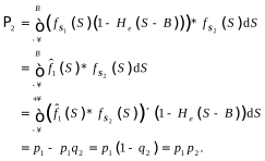
     <p><img width="315.97222222222223" src="https://html.scirp.org/file/1491194-rId365.svg?20250818023210">(11)</img></p>
     <p>
      <math xmlns="http://www.w3.org/1998/Math/MathML"> <mrow> 
        <msub> 
         <mover accent="true"> 
          <mi>
            f 
          </mi> 
          <mo>
            ^ 
          </mo> 
         </mover> 
         <mn>
           1 
         </mn> 
        </msub> 
        <mrow> 
         <mo>
           ( 
         </mo> 
         <mi>
           S 
         </mi> 
         <mo>
           ) 
         </mo> 
        </mrow> 
        <mo>
          ∗ 
        </mo> 
        <msub> 
         <mi>
           f 
         </mi> 
         <mrow> 
          <msub> 
           <mstyle mathvariant="bold" mathsize="normal"> 
            <mi>
              S 
            </mi> 
           </mstyle> 
           <mn>
             2 
           </mn> 
          </msub> 
         </mrow> 
        </msub> 
        <mrow> 
         <mo>
           ( 
         </mo> 
         <mi>
           S 
         </mi> 
         <mo>
           ) 
         </mo> 
        </mrow> 
       </mrow> 
      </math> is the convolution of the pdf’s 
      <math xmlns="http://www.w3.org/1998/Math/MathML"> <mrow> 
        <msub> 
         <mover accent="true"> 
          <mi>
            f 
          </mi> 
          <mo>
            ^ 
          </mo> 
         </mover> 
         <mn>
           1 
         </mn> 
        </msub> 
        <mrow> 
         <mo>
           ( 
         </mo> 
         <mi>
           S 
         </mi> 
         <mo>
           ) 
         </mo> 
        </mrow> 
       </mrow> 
      </math> and 
      <math xmlns="http://www.w3.org/1998/Math/MathML"> <mrow> 
        <msub> 
         <mi>
           f 
         </mi> 
         <mrow> 
          <msub> 
           <mstyle mathvariant="bold" mathsize="normal"> 
            <mi>
              S 
            </mi> 
           </mstyle> 
           <mn>
             2 
           </mn> 
          </msub> 
         </mrow> 
        </msub> 
        <mrow> 
         <mo>
           ( 
         </mo> 
         <mi>
           S 
         </mi> 
         <mo>
           ) 
         </mo> 
        </mrow> 
       </mrow> 
      </math>, and gives the pdf for the closing price of the second day for which the closing price of the first day did not exceed the barrier 
      <math xmlns="http://www.w3.org/1998/Math/MathML"> <mi>
         B 
       </mi> 
      </math>. The truncation of the pdf of the closing price for the previous day selects the “paths” for the time development of the closing price of the asset that do not cross the barrier. The approach presented here thus calculates the value of a path-dependent option without the need to simulate paths using a Monte Carlo approach.</p>
     <p>Note in Equation (11) that <img width="74.62039045553145" src="https://html.scirp.org/file/1491194-rId375.svg?20250818023210"> as expected since 
       <math xmlns="http://www.w3.org/1998/Math/MathML"> <mrow> 
         <msub> 
          <mi>
            p 
          </mi> 
          <mn>
            1 
          </mn> 
         </msub> 
        </mrow> 
       </math> and 
       <math xmlns="http://www.w3.org/1998/Math/MathML"> <mrow> 
         <msub> 
          <mi>
            p 
          </mi> 
          <mn>
            2 
          </mn> 
         </msub> 
        </mrow> 
       </math> are independent one-day probabilities that the price remained 
       <math xmlns="http://www.w3.org/1998/Math/MathML"> <mrow> 
         <mo>
           ≤ 
         </mo> 
         <mi>
           B 
         </mi> 
        </mrow> 
       </math>. The fact that </img></p>
     <p>
      <math xmlns="http://www.w3.org/1998/Math/MathML"> <mtable> 
        <mtr> 
         <mtd> 
          <msub> 
           <mi>
             p 
           </mi> 
           <mn>
             1 
           </mn> 
          </msub> 
          <msub> 
           <mi>
             q 
           </mi> 
           <mn>
             2 
           </mn> 
          </msub> 
          <mo>
            = 
          </mo> 
          <mstyle displaystyle="true"> 
           <mrow> 
            <munderover> 
             <mo>
               ∫ 
             </mo> 
             <mrow> 
              <mo>
                − 
              </mo> 
              <mi>
                ∞ 
              </mi> 
             </mrow> 
             <mrow> 
              <mo>
                + 
              </mo> 
              <mi>
                ∞ 
              </mi> 
             </mrow> 
            </munderover> 
            <mrow> 
             <mrow> 
              <mo>
                ( 
              </mo> 
              <mrow> 
               <msub> 
                <mover accent="true"> 
                 <mi>
                   f 
                 </mi> 
                 <mo>
                   ^ 
                 </mo> 
                </mover> 
                <mn>
                  1 
                </mn> 
               </msub> 
               <mrow> 
                <mo>
                  ( 
                </mo> 
                <mi>
                  S 
                </mi> 
                <mo>
                  ) 
                </mo> 
               </mrow> 
               <mo>
                 ∗ 
               </mo> 
               <msub> 
                <mi>
                  f 
                </mi> 
                <mrow> 
                 <msub> 
                  <mstyle mathsize="normal" mathvariant="bold"> 
                   <mi>
                     S 
                   </mi> 
                  </mstyle> 
                  <mn>
                    2 
                  </mn> 
                 </msub> 
                </mrow> 
               </msub> 
               <mrow> 
                <mo>
                  ( 
                </mo> 
                <mi>
                  S 
                </mi> 
                <mo>
                  ) 
                </mo> 
               </mrow> 
              </mrow> 
              <mo>
                ) 
              </mo> 
             </mrow> 
             <mo>
               × 
             </mo> 
             <mrow> 
              <mo>
                ( 
              </mo> 
              <mrow> 
               <msub> 
                <mi>
                  H 
                </mi> 
                <mi>
                  e 
                </mi> 
               </msub> 
               <mrow> 
                <mo>
                  ( 
                </mo> 
                <mrow> 
                 <mi>
                   S 
                 </mi> 
                 <mo>
                   − 
                 </mo> 
                 <mi>
                   B 
                 </mi> 
                </mrow> 
                <mo>
                  ) 
                </mo> 
               </mrow> 
              </mrow> 
              <mo>
                ) 
              </mo> 
             </mrow> 
             <mtext>
               d 
             </mtext> 
             <mi>
               S 
             </mi> 
            </mrow> 
           </mrow> 
          </mstyle> 
         </mtd> 
        </mtr> 
        <mtr> 
         <mtd> 
          <mo>
            = 
          </mo> 
          <mstyle displaystyle="true"> 
           <mrow> 
            <munderover> 
             <mo>
               ∫ 
             </mo> 
             <mi>
               B 
             </mi> 
             <mrow> 
              <mo>
                + 
              </mo> 
              <mi>
                ∞ 
              </mi> 
             </mrow> 
            </munderover> 
            <mrow> 
             <mrow> 
              <mo>
                ( 
              </mo> 
              <mrow> 
               <msub> 
                <mover accent="true"> 
                 <mi>
                   f 
                 </mi> 
                 <mo>
                   ^ 
                 </mo> 
                </mover> 
                <mn>
                  1 
                </mn> 
               </msub> 
               <mrow> 
                <mo>
                  ( 
                </mo> 
                <mi>
                  S 
                </mi> 
                <mo>
                  ) 
                </mo> 
               </mrow> 
               <mo>
                 ∗ 
               </mo> 
               <msub> 
                <mi>
                  f 
                </mi> 
                <mrow> 
                 <msub> 
                  <mstyle mathsize="normal" mathvariant="bold"> 
                   <mi>
                     S 
                   </mi> 
                  </mstyle> 
                  <mn>
                    2 
                  </mn> 
                 </msub> 
                </mrow> 
               </msub> 
               <mrow> 
                <mo>
                  ( 
                </mo> 
                <mi>
                  S 
                </mi> 
                <mo>
                  ) 
                </mo> 
               </mrow> 
              </mrow> 
              <mo>
                ) 
              </mo> 
             </mrow> 
             <mtext>
               d 
             </mtext> 
             <mi>
               S 
             </mi> 
            </mrow> 
           </mrow> 
          </mstyle> 
         </mtd> 
        </mtr> 
        <mtr> 
         <mtd> 
          <mo>
            = 
          </mo> 
          <mstyle displaystyle="true"> 
           <mrow> 
            <munderover> 
             <mo>
               ∫ 
             </mo> 
             <mi>
               B 
             </mi> 
             <mrow> 
              <mo>
                + 
              </mo> 
              <mi>
                ∞ 
              </mi> 
             </mrow> 
            </munderover> 
            <mrow> 
             <mstyle displaystyle="true"> 
              <mrow> 
               <munderover> 
                <mo>
                  ∫ 
                </mo> 
                <mrow> 
                 <mo>
                   − 
                 </mo> 
                 <mi>
                   ∞ 
                 </mi> 
                </mrow> 
                <mi>
                  B 
                </mi> 
               </munderover> 
               <mrow> 
                <mrow> 
                 <mo>
                   ( 
                 </mo> 
                 <mrow> 
                  <msub> 
                   <mover accent="true"> 
                    <mi>
                      f 
                    </mi> 
                    <mo>
                      ^ 
                    </mo> 
                   </mover> 
                   <mn>
                     1 
                   </mn> 
                  </msub> 
                  <mrow> 
                   <mo>
                     ( 
                   </mo> 
                   <mi>
                     u 
                   </mi> 
                   <mo>
                     ) 
                   </mo> 
                  </mrow> 
                  <msub> 
                   <mi>
                     f 
                   </mi> 
                   <mrow> 
                    <msub> 
                     <mstyle mathsize="normal" mathvariant="bold"> 
                      <mi>
                        S 
                      </mi> 
                     </mstyle> 
                     <mn>
                       2 
                     </mn> 
                    </msub> 
                   </mrow> 
                  </msub> 
                  <mrow> 
                   <mo>
                     ( 
                   </mo> 
                   <mrow> 
                    <mi>
                      S 
                    </mi> 
                    <mo>
                      − 
                    </mo> 
                    <mi>
                      u 
                    </mi> 
                   </mrow> 
                   <mo>
                     ) 
                   </mo> 
                  </mrow> 
                 </mrow> 
                 <mo>
                   ) 
                 </mo> 
                </mrow> 
                <mtext>
                  d 
                </mtext> 
                <mi>
                  u 
                </mi> 
                <mtext>
                  d 
                </mtext> 
                <mi>
                  S 
                </mi> 
               </mrow> 
              </mrow> 
             </mstyle> 
            </mrow> 
           </mrow> 
          </mstyle> 
         </mtd> 
        </mtr> 
       </mtable> 
      </math>(12)</p>
     <p>in Equations (11)-(12) is because 
      <math xmlns="http://www.w3.org/1998/Math/MathML"> <mrow> 
        <msub> 
         <mover accent="true"> 
          <mi>
            f 
          </mi> 
          <mo>
            ^ 
          </mo> 
         </mover> 
         <mn>
           1 
         </mn> 
        </msub> 
        <mrow> 
         <mo>
           ( 
         </mo> 
         <mi>
           S 
         </mi> 
         <mo>
           ) 
         </mo> 
        </mrow> 
        <mo>
          = 
        </mo> 
        <mn>
          0 
        </mn> 
        <mo>
          , 
        </mo> 
        <mi>
          S 
        </mi> 
        <mo>
          &gt; 
        </mo> 
        <mi>
          B 
        </mi> 
       </mrow> 
      </math>, the integral over the convolution is for 
      <math xmlns="http://www.w3.org/1998/Math/MathML"> <mrow> 
        <mi>
          S 
        </mi> 
        <mo>
          &gt; 
        </mo> 
        <mi>
          B 
        </mi> 
       </mrow> 
      </math>, and the support for 
      <math xmlns="http://www.w3.org/1998/Math/MathML"> <mrow> 
        <msub> 
         <mi>
           f 
         </mi> 
         <mrow> 
          <msub> 
           <mstyle mathvariant="bold" mathsize="normal"> 
            <mi>
              S 
            </mi> 
           </mstyle> 
           <mn>
             2 
           </mn> 
          </msub> 
         </mrow> 
        </msub> 
        <mrow> 
         <mo>
           ( 
         </mo> 
         <mi>
           S 
         </mi> 
         <mo>
           ) 
         </mo> 
        </mrow> 
       </mrow> 
      </math> includes the support for 
      <math xmlns="http://www.w3.org/1998/Math/MathML"> <mrow> 
        <msub> 
         <mover accent="true"> 
          <mi>
            f 
          </mi> 
          <mo>
            ^ 
          </mo> 
         </mover> 
         <mn>
           1 
         </mn> 
        </msub> 
        <mrow> 
         <mo>
           ( 
         </mo> 
         <mi>
           S 
         </mi> 
         <mo>
           ) 
         </mo> 
        </mrow> 
       </mrow> 
      </math> since the width of a convolution is greater than the widths of the functions.</p>
     <p>One method to obtain the result is to use the serial product method described by Bracewell (<xref ref-type="bibr" rid="scirp.144863-16">
       [16]
      </xref>, Ch. 3). Break the functions into small rectangles and follow one rectangle of 
      <math xmlns="http://www.w3.org/1998/Math/MathML"> <mrow> 
        <msub> 
         <mi>
           f 
         </mi> 
         <mrow> 
          <msub> 
           <mstyle mathvariant="bold" mathsize="normal"> 
            <mi>
              S 
            </mi> 
           </mstyle> 
           <mn>
             2 
           </mn> 
          </msub> 
         </mrow> 
        </msub> 
        <mrow> 
         <mo>
           ( 
         </mo> 
         <msup> 
          <mi>
            S 
          </mi> 
          <mo>
            ′ 
          </mo> 
         </msup> 
         <mo>
           ) 
         </mo> 
        </mrow> 
       </mrow> 
      </math> as it is swept across 
      <math xmlns="http://www.w3.org/1998/Math/MathML"> <mrow> 
        <msub> 
         <mover accent="true"> 
          <mi>
            f 
          </mi> 
          <mo>
            ^ 
          </mo> 
         </mover> 
         <mn>
           1 
         </mn> 
        </msub> 
        <mrow> 
         <mo>
           ( 
         </mo> 
         <mi>
           u 
         </mi> 
         <mo>
           ) 
         </mo> 
        </mrow> 
       </mrow> 
      </math> by the convolution. The rectangle of 
      <math xmlns="http://www.w3.org/1998/Math/MathML"> <mrow> 
        <msub> 
         <mi>
           f 
         </mi> 
         <mrow> 
          <msub> 
           <mstyle mathvariant="bold" mathsize="normal"> 
            <mi>
              S 
            </mi> 
           </mstyle> 
           <mn>
             2 
           </mn> 
          </msub> 
         </mrow> 
        </msub> 
        <mrow> 
         <mo>
           ( 
         </mo> 
         <msup> 
          <mi>
            S 
          </mi> 
          <mo>
            ′ 
          </mo> 
         </msup> 
         <mo>
           ) 
         </mo> 
        </mrow> 
       </mrow> 
      </math> is essentially a constant and can be taken outside of the integration over the dummy variable of integration 
      <math xmlns="http://www.w3.org/1998/Math/MathML"> <mi>
         u 
       </mi> 
      </math>. The integral over 
      <math xmlns="http://www.w3.org/1998/Math/MathML"> <mrow> 
        <msub> 
         <mover accent="true"> 
          <mi>
            f 
          </mi> 
          <mo>
            ^ 
          </mo> 
         </mover> 
         <mn>
           1 
         </mn> 
        </msub> 
        <mrow> 
         <mo>
           ( 
         </mo> 
         <mi>
           u 
         </mi> 
         <mo>
           ) 
         </mo> 
        </mrow> 
       </mrow> 
      </math> gives a contribution to 
      <math xmlns="http://www.w3.org/1998/Math/MathML"> <mrow> 
        <msub> 
         <mi>
           p 
         </mi> 
         <mn>
           1 
         </mn> 
        </msub> 
       </mrow> 
      </math> and the integral over 
      <math xmlns="http://www.w3.org/1998/Math/MathML"> <mi>
         S 
       </mi> 
      </math> gives a contribution to 
      <math xmlns="http://www.w3.org/1998/Math/MathML"> <mrow> 
        <msub> 
         <mi>
           q 
         </mi> 
         <mn>
           2 
         </mn> 
        </msub> 
       </mrow> 
      </math>.</p>
     <p>Let</p>
     <p>
      <math xmlns="http://www.w3.org/1998/Math/MathML"> <mrow> 
        <msub> 
         <mi>
           f 
         </mi> 
         <mrow> 
          <msub> 
           <mstyle mathvariant="bold" mathsize="normal"> 
            <mi>
              S 
            </mi> 
           </mstyle> 
           <mn>
             2 
           </mn> 
          </msub> 
         </mrow> 
        </msub> 
        <mrow> 
         <mo>
           ( 
         </mo> 
         <mrow> 
          <mi>
            S 
          </mi> 
          <mo>
            − 
          </mo> 
          <mi>
            u 
          </mi> 
         </mrow> 
         <mo>
           ) 
         </mo> 
        </mrow> 
        <mo>
          = 
        </mo> 
        <mstyle displaystyle="true"> 
         <munder> 
          <mo>
            ∑ 
          </mo> 
          <mi>
            j 
          </mi> 
         </munder> 
         <mrow> 
          <msub> 
           <mover accent="true"> 
            <mi>
              f 
            </mi> 
            <mo>
              ¯ 
            </mo> 
           </mover> 
           <mn>
             2 
           </mn> 
          </msub> 
          <mrow> 
           <mo>
             ( 
           </mo> 
           <mrow> 
            <msub> 
             <msup> 
              <mi>
                S 
              </mi> 
              <mo>
                ′ 
              </mo> 
             </msup> 
             <mi>
               j 
             </mi> 
            </msub> 
           </mrow> 
           <mo>
             ) 
           </mo> 
          </mrow> 
         </mrow> 
        </mstyle> 
       </mrow> 
      </math>(13)</p>
     <p>
      <xref ref-type="bibr" rid="scirp.144863-"></xref>where 
      <math xmlns="http://www.w3.org/1998/Math/MathML"> <mrow> 
        <msub> 
         <mover accent="true"> 
          <mi>
            f 
          </mi> 
          <mo>
            ¯ 
          </mo> 
         </mover> 
         <mn>
           2 
         </mn> 
        </msub> 
        <mrow> 
         <mo>
           ( 
         </mo> 
         <mrow> 
          <msub> 
           <msup> 
            <mi>
              S 
            </mi> 
            <mo>
              ′ 
            </mo> 
           </msup> 
           <mi>
             j 
           </mi> 
          </msub> 
         </mrow> 
         <mo>
           ) 
         </mo> 
        </mrow> 
       </mrow> 
      </math> is composed of contiguous rectangles of small width such that 
      <math xmlns="http://www.w3.org/1998/Math/MathML"> <mrow> 
        <msub> 
         <mover accent="true"> 
          <mi>
            f 
          </mi> 
          <mo>
            ¯ 
          </mo> 
         </mover> 
         <mn>
           2 
         </mn> 
        </msub> 
        <mrow> 
         <mo>
           ( 
         </mo> 
         <mrow> 
          <msub> 
           <msup> 
            <mi>
              S 
            </mi> 
            <mo>
              ′ 
            </mo> 
           </msup> 
           <mi>
             j 
           </mi> 
          </msub> 
         </mrow> 
         <mo>
           ) 
         </mo> 
        </mrow> 
       </mrow> 
      </math> is essentially constant with respect to 
      <math xmlns="http://www.w3.org/1998/Math/MathML"> <mi>
         S 
       </mi> 
      </math> and 
      <math xmlns="http://www.w3.org/1998/Math/MathML"> <mi>
         u 
       </mi> 
      </math> over the width of the rectangle.</p>
     <p>In the integral definition of the convolution, such as Equation (1), 
      <math xmlns="http://www.w3.org/1998/Math/MathML"> <mi>
         x 
       </mi> 
      </math> is a parameter chosen by the user; it is the point for which the user wishes to know the convolution. In the last line of Equation (12), the parameter for the convolution is 
      <math xmlns="http://www.w3.org/1998/Math/MathML"> <mi>
         S 
       </mi> 
      </math>. Chose 
      <math xmlns="http://www.w3.org/1998/Math/MathML"> <mi>
         S 
       </mi> 
      </math> such that 
      <math xmlns="http://www.w3.org/1998/Math/MathML"> <mrow> 
        <msub> 
         <mi>
           f 
         </mi> 
         <mrow> 
          <msub> 
           <mstyle mathvariant="bold" mathsize="normal"> 
            <mi>
              S 
            </mi> 
           </mstyle> 
           <mn>
             2 
           </mn> 
          </msub> 
         </mrow> 
        </msub> 
        <mrow> 
         <mo>
           ( 
         </mo> 
         <mrow> 
          <mi>
            S 
          </mi> 
          <mo>
            − 
          </mo> 
          <mi>
            u 
          </mi> 
         </mrow> 
         <mo>
           ) 
         </mo> 
        </mrow> 
       </mrow> 
      </math> is constant over the integral 
      <math xmlns="http://www.w3.org/1998/Math/MathML"> <mrow> 
        <mstyle displaystyle="true"> 
         <mrow> 
          <mo>
            ∫ 
          </mo> 
          <mrow> 
           <msub> 
            <mover accent="true"> 
             <mi>
               f 
             </mi> 
             <mo>
               ^ 
             </mo> 
            </mover> 
            <mn>
              1 
            </mn> 
           </msub> 
           <mrow> 
            <mo>
              ( 
            </mo> 
            <mi>
              u 
            </mi> 
            <mo>
              ) 
            </mo> 
           </mrow> 
           <mo> 
           </mo> 
           <mtext>
             d 
           </mtext> 
           <mi>
             u 
           </mi> 
          </mrow> 
         </mrow> 
        </mstyle> 
       </mrow> 
      </math>. If this choice is made, then</p>
     <p>
      <math xmlns="http://www.w3.org/1998/Math/MathML"> <mtable> 
        <mtr> 
         <mtd> 
          <msub> 
           <mi>
             p 
           </mi> 
           <mn>
             1 
           </mn> 
          </msub> 
          <msub> 
           <mi>
             q 
           </mi> 
           <mn>
             2 
           </mn> 
          </msub> 
          <mo>
            = 
          </mo> 
          <mstyle displaystyle="true"> 
           <mrow> 
            <munderover> 
             <mo>
               ∫ 
             </mo> 
             <mi>
               B 
             </mi> 
             <mrow> 
              <mo>
                + 
              </mo> 
              <mi>
                ∞ 
              </mi> 
             </mrow> 
            </munderover> 
            <mrow> 
             <mrow> 
              <mo>
                ( 
              </mo> 
              <mrow> 
               <msub> 
                <mover accent="true"> 
                 <mi>
                   f 
                 </mi> 
                 <mo>
                   ^ 
                 </mo> 
                </mover> 
                <mn>
                  1 
                </mn> 
               </msub> 
               <mrow> 
                <mo>
                  ( 
                </mo> 
                <mi>
                  S 
                </mi> 
                <mo>
                  ) 
                </mo> 
               </mrow> 
               <mo>
                 ∗ 
               </mo> 
               <msub> 
                <mi>
                  f 
                </mi> 
                <mrow> 
                 <msub> 
                  <mstyle mathsize="normal" mathvariant="bold"> 
                   <mi>
                     S 
                   </mi> 
                  </mstyle> 
                  <mn>
                    2 
                  </mn> 
                 </msub> 
                </mrow> 
               </msub> 
               <mrow> 
                <mo>
                  ( 
                </mo> 
                <mi>
                  S 
                </mi> 
                <mo>
                  ) 
                </mo> 
               </mrow> 
              </mrow> 
              <mo>
                ) 
              </mo> 
             </mrow> 
             <mtext>
               d 
             </mtext> 
             <mi>
               S 
             </mi> 
            </mrow> 
           </mrow> 
          </mstyle> 
         </mtd> 
        </mtr> 
        <mtr> 
         <mtd> 
          <mo>
            = 
          </mo> 
          <mstyle displaystyle="true"> 
           <munder> 
            <mo>
              ∑ 
            </mo> 
            <mi>
              j 
            </mi> 
           </munder> 
           <mrow> 
            <mstyle displaystyle="true"> 
             <mrow> 
              <munderover> 
               <mo>
                 ∫ 
               </mo> 
               <mi>
                 B 
               </mi> 
               <mrow> 
                <mo>
                  + 
                </mo> 
                <mi>
                  ∞ 
                </mi> 
               </mrow> 
              </munderover> 
              <mrow> 
               <mstyle displaystyle="true"> 
                <mrow> 
                 <munderover> 
                  <mo>
                    ∫ 
                  </mo> 
                  <mrow> 
                   <mo>
                     − 
                   </mo> 
                   <mi>
                     ∞ 
                   </mi> 
                  </mrow> 
                  <mi>
                    B 
                  </mi> 
                 </munderover> 
                 <mrow> 
                  <mrow> 
                   <mo>
                     ( 
                   </mo> 
                   <mrow> 
                    <msub> 
                     <mover accent="true"> 
                      <mi>
                        f 
                      </mi> 
                      <mo>
                        ^ 
                      </mo> 
                     </mover> 
                     <mn>
                       1 
                     </mn> 
                    </msub> 
                    <mrow> 
                     <mo>
                       ( 
                     </mo> 
                     <mi>
                       u 
                     </mi> 
                     <mo>
                       ) 
                     </mo> 
                    </mrow> 
                    <msub> 
                     <mover accent="true"> 
                      <mi>
                        f 
                      </mi> 
                      <mo>
                        ¯ 
                      </mo> 
                     </mover> 
                     <mn>
                       2 
                     </mn> 
                    </msub> 
                    <mrow> 
                     <mo>
                       ( 
                     </mo> 
                     <mrow> 
                      <msub> 
                       <msup> 
                        <mi>
                          S 
                        </mi> 
                        <mo>
                          ′ 
                        </mo> 
                       </msup> 
                       <mi>
                         j 
                       </mi> 
                      </msub> 
                     </mrow> 
                     <mo>
                       ) 
                     </mo> 
                    </mrow> 
                   </mrow> 
                   <mo>
                     ) 
                   </mo> 
                  </mrow> 
                  <mtext>
                    d 
                  </mtext> 
                  <mi>
                    u 
                  </mi> 
                  <mtext>
                    d 
                  </mtext> 
                  <mi>
                    S 
                  </mi> 
                 </mrow> 
                </mrow> 
               </mstyle> 
              </mrow> 
             </mrow> 
            </mstyle> 
           </mrow> 
          </mstyle> 
         </mtd> 
        </mtr> 
        <mtr> 
         <mtd> 
          <mo>
            = 
          </mo> 
          <mstyle displaystyle="true"> 
           <munder> 
            <mo>
              ∑ 
            </mo> 
            <mi>
              j 
            </mi> 
           </munder> 
           <mrow> 
            <msub> 
             <mi>
               p 
             </mi> 
             <mn>
               1 
             </mn> 
            </msub> 
            <msub> 
             <mi>
               q 
             </mi> 
             <mn>
               2 
             </mn> 
            </msub> 
            <msub> 
             <mrow /> 
             <mi>
               j 
             </mi> 
            </msub> 
           </mrow> 
          </mstyle> 
          <mo>
            = 
          </mo> 
          <msub> 
           <mi>
             p 
           </mi> 
           <mn>
             1 
           </mn> 
          </msub> 
          <msub> 
           <mi>
             q 
           </mi> 
           <mn>
             2 
           </mn> 
          </msub> 
          <mo>
            . 
          </mo> 
         </mtd> 
        </mtr> 
       </mtable> 
      </math>(14)</p>
     <p>
      <math xmlns="http://www.w3.org/1998/Math/MathML"> <mrow> 
        <msub> 
         <mover accent="true"> 
          <mi>
            f 
          </mi> 
          <mo>
            ^ 
          </mo> 
         </mover> 
         <mn>
           2 
         </mn> 
        </msub> 
        <mrow> 
         <mo>
           ( 
         </mo> 
         <mi>
           S 
         </mi> 
         <mo>
           ) 
         </mo> 
        </mrow> 
       </mrow> 
      </math> is defined in a similar manner to 
      <math xmlns="http://www.w3.org/1998/Math/MathML"> <mrow> 
        <msub> 
         <mover accent="true"> 
          <mi>
            f 
          </mi> 
          <mo>
            ^ 
          </mo> 
         </mover> 
         <mn>
           1 
         </mn> 
        </msub> 
        <mrow> 
         <mo>
           ( 
         </mo> 
         <mi>
           S 
         </mi> 
         <mo>
           ) 
         </mo> 
        </mrow> 
       </mrow> 
      </math>, with 
      <math xmlns="http://www.w3.org/1998/Math/MathML"> <mrow> 
        <msub> 
         <mover accent="true"> 
          <mi>
            f 
          </mi> 
          <mo>
            ^ 
          </mo> 
         </mover> 
         <mn>
           2 
         </mn> 
        </msub> 
        <mrow> 
         <mo>
           ( 
         </mo> 
         <mi>
           S 
         </mi> 
         <mo>
           ) 
         </mo> 
        </mrow> 
       </mrow> 
      </math> the truncation of a convolution</p>
     <p>
      <math xmlns="http://www.w3.org/1998/Math/MathML"> <mrow> 
        <msub> 
         <mover accent="true"> 
          <mi>
            f 
          </mi> 
          <mo>
            ^ 
          </mo> 
         </mover> 
         <mn>
           2 
         </mn> 
        </msub> 
        <mrow> 
         <mo>
           ( 
         </mo> 
         <mi>
           S 
         </mi> 
         <mo>
           ) 
         </mo> 
        </mrow> 
        <mo>
          = 
        </mo> 
        <mrow> 
         <mo>
           ( 
         </mo> 
         <mrow> 
          <msub> 
           <mover accent="true"> 
            <mi>
              f 
            </mi> 
            <mo>
              ^ 
            </mo> 
           </mover> 
           <mn>
             1 
           </mn> 
          </msub> 
          <mrow> 
           <mo>
             ( 
           </mo> 
           <mi>
             S 
           </mi> 
           <mo>
             ) 
           </mo> 
          </mrow> 
          <mo>
            ∗ 
          </mo> 
          <msub> 
           <mi>
             f 
           </mi> 
           <mrow> 
            <msub> 
             <mstyle mathvariant="bold" mathsize="normal"> 
              <mi>
                S 
              </mi> 
             </mstyle> 
             <mn>
               2 
             </mn> 
            </msub> 
           </mrow> 
          </msub> 
          <mrow> 
           <mo>
             ( 
           </mo> 
           <mi>
             S 
           </mi> 
           <mo>
             ) 
           </mo> 
          </mrow> 
         </mrow> 
         <mo>
           ) 
         </mo> 
        </mrow> 
        <mo>
          × 
        </mo> 
        <mrow> 
         <mo>
           ( 
         </mo> 
         <mrow> 
          <mn>
            1 
          </mn> 
          <mo>
            − 
          </mo> 
          <msub> 
           <mi>
             H 
           </mi> 
           <mi>
             e 
           </mi> 
          </msub> 
          <mrow> 
           <mo>
             ( 
           </mo> 
           <mrow> 
            <mi>
              S 
            </mi> 
            <mo>
              − 
            </mo> 
            <mi>
              B 
            </mi> 
           </mrow> 
           <mo>
             ) 
           </mo> 
          </mrow> 
         </mrow> 
         <mo>
           ) 
         </mo> 
        </mrow> 
        <mo>
          , 
        </mo> 
       </mrow> 
      </math>(15)</p>
     <p>which leads to general expressions for 
      <math xmlns="http://www.w3.org/1998/Math/MathML"> <mrow> 
        <msub> 
         <mover accent="true"> 
          <mi>
            f 
          </mi> 
          <mo>
            ^ 
          </mo> 
         </mover> 
         <mi>
           i 
         </mi> 
        </msub> 
       </mrow> 
      </math>, 
      <math xmlns="http://www.w3.org/1998/Math/MathML"> <mrow> 
        <msub> 
         <mi>
           p 
         </mi> 
         <mi>
           i 
         </mi> 
        </msub> 
       </mrow> 
      </math>, and <img width="104.12147505422993" src="https://html.scirp.org/file/1491194-rId442.svg?20250818023210">, where 
       <math xmlns="http://www.w3.org/1998/Math/MathML"> <mi>
          i 
        </mi> 
       </math>, 
       <math xmlns="http://www.w3.org/1998/Math/MathML"> <mrow> 
         <mi>
           i 
         </mi> 
         <mo>
           &gt; 
         </mo> 
         <mn>
           1 
         </mn> 
        </mrow> 
       </math>, is the 
       <math xmlns="http://www.w3.org/1998/Math/MathML"> <mrow> 
         <msup> 
          <mi>
            i 
          </mi> 
          <mrow> 
           <mtext>
             th 
           </mtext> 
          </mrow> 
         </msup> 
        </mrow> 
       </math> day of an n-day option, and thus to the ability to price a barrier option. The required pdf’s are built by sequentially convolving and truncating: </img></p>
     <p>
      <math xmlns="http://www.w3.org/1998/Math/MathML"> <mrow> 
        <msub> 
         <mover accent="true"> 
          <mi>
            f 
          </mi> 
          <mo>
            ^ 
          </mo> 
         </mover> 
         <mi>
           i 
         </mi> 
        </msub> 
        <mrow> 
         <mo>
           ( 
         </mo> 
         <mi>
           S 
         </mi> 
         <mo>
           ) 
         </mo> 
        </mrow> 
        <mo>
          = 
        </mo> 
        <mrow> 
         <mo>
           ( 
         </mo> 
         <mrow> 
          <msub> 
           <mover accent="true"> 
            <mi>
              f 
            </mi> 
            <mo>
              ^ 
            </mo> 
           </mover> 
           <mrow> 
            <mi>
              i 
            </mi> 
            <mo>
              − 
            </mo> 
            <mn>
              1 
            </mn> 
           </mrow> 
          </msub> 
          <mrow> 
           <mo>
             ( 
           </mo> 
           <mi>
             S 
           </mi> 
           <mo>
             ) 
           </mo> 
          </mrow> 
          <mo>
            ∗ 
          </mo> 
          <msub> 
           <mi>
             f 
           </mi> 
           <mrow> 
            <msub> 
             <mstyle mathvariant="bold" mathsize="normal"> 
              <mi>
                S 
              </mi> 
             </mstyle> 
             <mi>
               i 
             </mi> 
            </msub> 
           </mrow> 
          </msub> 
          <mrow> 
           <mo>
             ( 
           </mo> 
           <mi>
             S 
           </mi> 
           <mo>
             ) 
           </mo> 
          </mrow> 
         </mrow> 
         <mo>
           ) 
         </mo> 
        </mrow> 
        <mo>
          × 
        </mo> 
        <mrow> 
         <mo>
           ( 
         </mo> 
         <mrow> 
          <mn>
            1 
          </mn> 
          <mo>
            − 
          </mo> 
          <msub> 
           <mi>
             H 
           </mi> 
           <mi>
             e 
           </mi> 
          </msub> 
          <mrow> 
           <mo>
             ( 
           </mo> 
           <mrow> 
            <mi>
              S 
            </mi> 
            <mo>
              − 
            </mo> 
            <mi>
              B 
            </mi> 
           </mrow> 
           <mo>
             ) 
           </mo> 
          </mrow> 
         </mrow> 
         <mo>
           ) 
         </mo> 
        </mrow> 
       </mrow> 
      </math>(16)</p>
     <p><img width="284.72222222222223" src="https://html.scirp.org/file/1491194-rId452.svg?20250818023210">(17)</img></p>
     <p>If it is assumed that the one-day returns are stationary in that the distribution of returns is the same for each day that the option is alive, then the notation can be simplified as 
      <math xmlns="http://www.w3.org/1998/Math/MathML"> <mrow> 
        <mstyle mathvariant="bold" mathsize="normal"> 
         <mi>
           S 
         </mi> 
        </mstyle> 
        <mo>
          = 
        </mo> 
        <msub> 
         <mstyle mathvariant="bold" mathsize="normal"> 
          <mi>
            S 
          </mi> 
         </mstyle> 
         <mi>
           i 
         </mi> 
        </msub> 
       </mrow> 
      </math> for all 
      <math xmlns="http://www.w3.org/1998/Math/MathML"> <mi>
         i 
       </mi> 
      </math>. In this case <img width="126.68112798264642" src="https://html.scirp.org/file/1491194-rId458.svg?20250818023210"> where 
       <math xmlns="http://www.w3.org/1998/Math/MathML"> <mrow> 
         <mi>
           p 
         </mi> 
         <mo>
           = 
         </mo> 
         <mstyle displaystyle="true"> 
          <mrow> 
           <msubsup> 
            <mo>
              ∫ 
            </mo> 
            <mrow> 
             <mo>
               − 
             </mo> 
             <mi>
               ∞ 
             </mi> 
            </mrow> 
            <mi>
              B 
            </mi> 
           </msubsup> 
           <mrow> 
            <msub> 
             <mi>
               f 
             </mi> 
             <mstyle mathvariant="bold" mathsize="normal"> 
              <mi>
                S 
              </mi> 
             </mstyle> 
            </msub> 
            <mrow> 
             <mo>
               ( 
             </mo> 
             <mi>
               S 
             </mi> 
             <mo>
               ) 
             </mo> 
            </mrow> 
            <mtext>
              d 
            </mtext> 
            <mi>
              S 
            </mi> 
           </mrow> 
          </mrow> 
         </mstyle> 
        </mrow> 
       </math> is the probability of crossing the barrier on any single day. <img width="20.824295010845987" src="https://html.scirp.org/file/1491194-rId462.svg?20250818023210"> gives the probability that the option has not crossed the barrier at the beginning of the 
        <math xmlns="http://www.w3.org/1998/Math/MathML"> <mrow> 
          <msup> 
           <mrow> 
            <mrow> 
             <mo>
               ( 
             </mo> 
             <mrow> 
              <mi>
                i 
              </mi> 
              <mo>
                + 
              </mo> 
              <mn>
                1 
              </mn> 
             </mrow> 
             <mo>
               ) 
             </mo> 
            </mrow> 
           </mrow> 
           <mrow> 
            <mtext>
              th 
            </mtext> 
           </mrow> 
          </msup> 
         </mrow> 
        </math> interval.</img></img></p>
     <p>There is no need for Monte Carlo simulation of 
      <math xmlns="http://www.w3.org/1998/Math/MathML"> <mstyle mathvariant="bold" mathsize="normal"> 
        <mi>
          S 
        </mi> 
       </mstyle> 
      </math> to find the price of a barrier option; there is no need to analyse an ensemble of calculated paths to find probabilities. n-fold truncation and convolution of the one-day distribution gives the n-day return pdf as a sequence of uniformly sampled numbers. This pdf as a sequence of numbers can be integrated to find the probabilities and expectations required to price options. The pdf also does not contain random fluctuations and non-uniform coverage owing to draws from a random number generator.</p>
     <p>Drift is handled in a straightforward manner with the method of repeated convolution and truncation of the pdfs for the adjusted closing value. 
      <math xmlns="http://www.w3.org/1998/Math/MathML"> <mrow> 
        <msub> 
         <mi>
           f 
         </mi> 
         <mrow> 
          <mi>
            i 
          </mi> 
          <mo>
            + 
          </mo> 
          <mn>
            1 
          </mn> 
         </mrow> 
        </msub> 
        <mrow> 
         <mo>
           ( 
         </mo> 
         <mi>
           S 
         </mi> 
         <mo>
           ) 
         </mo> 
        </mrow> 
       </mrow> 
      </math> contains the memory of all drift from the previous 
      <math xmlns="http://www.w3.org/1998/Math/MathML"> <mi>
         i 
       </mi> 
      </math> days. Note that 
      <math xmlns="http://www.w3.org/1998/Math/MathML"> <mrow> 
        <msub> 
         <mi>
           α 
         </mi> 
         <mi>
           i 
         </mi> 
        </msub> 
       </mrow> 
      </math>, the rate of drift for each time interval, need not be same for each day. Similarly, different pdf’s could be used for each interval of time, which is a day in this work.</p>
     <p>
      <xref ref-type="fig" rid="fig2">
       Figure 2
      </xref> is composed of semi- 
      <math xmlns="http://www.w3.org/1998/Math/MathML"> <mrow> 
        <msub> 
         <mrow> 
          <mtext>
            log 
          </mtext> 
         </mrow> 
         <mrow> 
          <mn>
            10 
          </mn> 
         </mrow> 
        </msub> 
       </mrow> 
      </math> plots of the pdfs for the closing value of the asset 
      <math xmlns="http://www.w3.org/1998/Math/MathML"> <mi>
         S 
       </mi> 
      </math> based on best fits of a normal distribution (black) and the best-fit t+ distribution (i.e., the sum of a Student’s t distribution plus a Gaussian distribution) (red) to the one-day returns for the S&amp;P 500. The convolution of a one-day barrier-truncated t+ distribution (shown in red to the left of the green line) with the one-day closing value (the full red curve) is shown in blue. The barrier truncation was for values 
      <math xmlns="http://www.w3.org/1998/Math/MathML"> <mrow> 
        <mo>
          &gt; 
        </mo> 
        <mi>
          B 
        </mi> 
        <mo>
          = 
        </mo> 
        <mtext>
          $ 
        </mtext> 
        <mn>
          53.00 
        </mn> 
       </mrow> 
      </math>. The truncation of the blue curve at the barrier level is shown in green. The area under the blue curve to the left of the green line gives the probability that the closing value after two days will be 
      <math xmlns="http://www.w3.org/1998/Math/MathML"> <mrow> 
        <mo>
          ≤ 
        </mo> 
        <mi>
          B 
        </mi> 
       </mrow> 
      </math>.</p>
     <p>The convolutions were calculated numerically. In the calculation of the convolution, any final results that were &lt;10<sup>−</sup><sup>7</sup> were set to zero. This reduces the amount of storage and the time that are required to calculate the convolutions while keeping the uncertainty ≈10<sup>−</sup><sup>5</sup> for calculation of the closing value after 100 days. The steep roll-off in the wings of the blue curve (which is visible on the right-hand side) shows that there is negligible area in the truncation for values of 
      <math xmlns="http://www.w3.org/1998/Math/MathML"> <mi>
         S 
       </mi> 
      </math> that occur with the pdf having a value &lt; 10<sup>−</sup><sup>7</sup>. Nevertheless, the pdf after the 
      <math xmlns="http://www.w3.org/1998/Math/MathML"> <mrow> 
        <msup> 
         <mi>
           i 
         </mi> 
         <mrow> 
          <mtext>
            th 
          </mtext> 
         </mrow> 
        </msup> 
       </mrow> 
      </math> convolution and before truncation at the barrier value was renormalised to the value of <img width="29.488291413703383" src="https://html.scirp.org/file/1491194-rId486.svg?20250818023210"> to avoid accumulation of the loss of probability through truncation of final results that were &lt;10<sup>−</sup><sup>7</sup>.</img></p>
     <p>The pdfs for the one-day (red) and two-day (blue) closing values of the asset are truncated (as discussed in the preceding paragraph), although not as harshly as the barrier truncation shown in <xref ref-type="fig" rid="fig2">
       Figure 2
      </xref>. The truncations for the red and blue curves are shown only on the left-hand side as vertical lines. The other truncations are not shown to avoid visual distraction. Nevertheless, repeated convolution of the truncated one-day pdf leads rapidly to a normal-like distribution <xref ref-type="bibr" rid="scirp.144863-24">
       [24]
      </xref>. This truncation of the pdf is physical and necessary to price options with fat tails <xref ref-type="bibr" rid="scirp.144863-23">
       [23]
      </xref> <xref ref-type="bibr" rid="scirp.144863-34">
       [34]
      </xref>. This is argued in Section 2.2 and also shown in Appendix A.</p>
     <p>The best-fit t+ distribution to the one-day returns was truncated to the interval 
      <math xmlns="http://www.w3.org/1998/Math/MathML"> <mrow> 
        <mrow> 
         <mo>
           [ 
         </mo> 
         <mrow> 
          <msub> 
           <mi>
             S 
           </mi> 
           <mn>
             0 
           </mn> 
          </msub> 
          <mo>
            − 
          </mo> 
          <mn>
            14.13 
          </mn> 
          <mo>
            , 
          </mo> 
          <msub> 
           <mi>
             S 
           </mi> 
           <mn>
             0 
           </mn> 
          </msub> 
          <mo>
            + 
          </mo> 
          <mn>
            7.05 
          </mn> 
         </mrow> 
         <mo>
           ] 
         </mo> 
        </mrow> 
       </mrow> 
      </math> such that the minimum return of −229‰ and the maximum return of 109.6‰ were included. The interval 
      <math xmlns="http://www.w3.org/1998/Math/MathML"> <mrow> 
        <mrow> 
         <mo>
           [ 
         </mo> 
         <mrow> 
          <msub> 
           <mi>
             S 
           </mi> 
           <mn>
             0 
           </mn> 
          </msub> 
          <mo>
            − 
          </mo> 
          <mn>
            14.13 
          </mn> 
          <mo>
            , 
          </mo> 
          <msub> 
           <mi>
             S 
           </mi> 
           <mn>
             0 
           </mn> 
          </msub> 
          <mo>
            + 
          </mo> 
          <mn>
            7.05 
          </mn> 
         </mrow> 
         <mo>
           ] 
         </mo> 
        </mrow> 
       </mrow> 
      </math> corresponds to per mille returns of 
      <math xmlns="http://www.w3.org/1998/Math/MathML"> <mrow> 
        <mrow> 
         <mo>
           [ 
         </mo> 
         <mrow> 
          <mo>
            − 
          </mo> 
          <mn>
            332.1 
          </mn> 
          <mo>
            , 
          </mo> 
          <mn>
            13.19 
          </mn> 
         </mrow> 
         <mo>
           ] 
         </mo> 
        </mrow> 
       </mrow> 
      </math>. Option prices for assets with returns that follow a Student’s t distribution or other fat-tailed distribution can be obtained if the distributions are truncated or the return is capped <xref ref-type="bibr" rid="scirp.144863-23">
       [23]
      </xref> <xref ref-type="bibr" rid="scirp.144863-28">
       [28]
      </xref> <xref ref-type="bibr" rid="scirp.144863-29">
       [29]
      </xref> <xref ref-type="bibr" rid="scirp.144863-34">
       [34]
      </xref>. Truncation of the pdf was chosen.</p>
     <fig id="fig2" position="float">
      <label>Figure 2</label>
      <caption>
       <title>Figure 2. Plots of probability density functions (pdf’s) for values of 

        <math xmlns="http://www.w3.org/1998/Math/MathML"> <mi>
          
  S
 
         </mi>

        </math> as a function of distance from 

        <math xmlns="http://www.w3.org/1998/Math/MathML"> <mrow> 
  
          <msub> 
   
           <mi>
            
    S
   
           </mi> 
   
           <mn>
            
    0
   
           </mn> 
  
          </msub> 
  
          <mo>
           
   =
  
          </mo>
  
          <mn>
           
   50
  
          </mn>
 
         </mrow>

        </math>. Best-fit pdfs to one-day returns, 

        <math xmlns="http://www.w3.org/1998/Math/MathML"> <mrow> 
  
          <msub> 
   
           <mi>
            
    f
   
           </mi> 
   
           <mrow> 
    
            <msub> 
     
             <mstyle mathvariant="bold" mathsize="normal"> 
              <mi>
                S 
              </mi> 
             </mstyle> 
     
             <mn>
               1 
             </mn> 
    
            </msub> 
   
           </mrow> 
  
          </msub> 
  
          <mrow>
   
           <mo>
            
    (
   
           </mo> 
   
           <mi>
            
    S
   
           </mi> 
   
           <mo>
            
    )
   
           </mo>
  
          </mrow>
 
         </mrow>

        </math>, for normal (black) and for t+ (red) distributions to the S&amp;P 500. The curves in grey (normal distribution) and blue (t+ distribution) display the predicted pdf’s for two-day returns, 

        <math xmlns="http://www.w3.org/1998/Math/MathML"> <mrow> 
  
          <msub> 
   
           <mi>
            
    f
   
           </mi> 
   
           <mrow> 
    
            <msub> 
     
             <mstyle mathvariant="bold" mathsize="normal"> 
              <mi>
                S 
              </mi> 
             </mstyle> 
     
             <mn>
               2 
             </mn> 
    
            </msub> 
   
           </mrow> 
  
          </msub> 
  
          <mrow>
   
           <mo>
            
    (
   
           </mo> 
   
           <mi>
            
    S
   
           </mi> 
   
           <mo>
            
    )
   
           </mo>
  
          </mrow>
 
         </mrow>

        </math>, based on convolutions 

        <math xmlns="http://www.w3.org/1998/Math/MathML"> <mrow> 
  
          <msub> 
   
           <mover accent="true"> 
    
            <mi>
             
     f
    
            </mi> 
    
            <mo>
             
     ^
    
            </mo> 
   
           </mover> 
   
           <mn>
            
    1
   
           </mn> 
  
          </msub> 
  
          <mrow>
   
           <mo>
            
    (
   
           </mo> 
   
           <mi>
            
    S
   
           </mi> 
   
           <mo>
            
    )
   
           </mo>
  
          </mrow>
  
          <mo>
           
   ∗
  
          </mo>
  
          <msub> 
   
           <mi>
            
    f
   
           </mi> 
   
           <mrow> 
    
            <msub> 
     
             <mstyle mathvariant="bold" mathsize="normal"> 
              <mi>
                S 
              </mi> 
             </mstyle> 
     
             <mn>
               2 
             </mn> 
    
            </msub> 
   
           </mrow> 
  
          </msub> 
  
          <mrow>
   
           <mo>
            
    (
   
           </mo> 
   
           <mi>
            
    S
   
           </mi> 
   
           <mo>
            
    )
   
           </mo>
  
          </mrow>
 
         </mrow>

        </math>. Areas to the left of the green line and under the pdf’s give the probability for the value of 

        <math xmlns="http://www.w3.org/1998/Math/MathML"> <mi>
          
  S
 
         </mi>

        </math> to remain below the barrier of 53. 

        <math xmlns="http://www.w3.org/1998/Math/MathML"> <mrow> 
  
          <msub> 
   
           <mover accent="true"> 
    
            <mi>
             
     f
    
            </mi> 
    
            <mo>
             
     ^
    
            </mo> 
   
           </mover> 
   
           <mn>
            
    1
   
           </mn> 
  
          </msub> 
  
          <mrow>
   
           <mo>
            
    (
   
           </mo> 
   
           <mi>
            
    S
   
           </mi> 
   
           <mo>
            
    )
   
           </mo>
  
          </mrow>
 
         </mrow>

        </math> is the red curve to the left of the vertical, green line. 

        <math xmlns="http://www.w3.org/1998/Math/MathML"> <mrow> 
  
          <msub> 
   
           <mover accent="true"> 
    
            <mi>
             
     f
    
            </mi> 
    
            <mo>
             
     ^
    
            </mo> 
   
           </mover> 
   
           <mn>
            
    2
   
           </mn> 
  
          </msub> 
  
          <mrow>
   
           <mo>
            
    (
   
           </mo> 
   
           <mi>
            
    S
   
           </mi> 
   
           <mo>
            
    )
   
           </mo>
  
          </mrow>
 
         </mrow>

        </math> is the blue curve to the left of the vertical, green line.</title>
      </caption>
      <graphic mimetype="image" position="float" xlink:type="simple" xlink:href="https://html.scirp.org/file/1491194-rId494.jpeg?20250818023210" />
     </fig>
     <p>
      <xref ref-type="table" rid="table1">
       Table 1
      </xref> lists the probabilities <img width="112.84722222222223" src="https://html.scirp.org/file/1491194-rId511.svg?20250818023210"> that the closing prices of the asset are all below a barrier 
       <math xmlns="http://www.w3.org/1998/Math/MathML"> <mi>
          B 
        </mi> 
       </math> for 
       <math xmlns="http://www.w3.org/1998/Math/MathML"> <mi>
          T 
        </mi> 
       </math> closing days for three values of the barrier. The initial price of the asset was assumed to be 
       <math xmlns="http://www.w3.org/1998/Math/MathML"> <mrow> 
         <msub> 
          <mi>
            S 
          </mi> 
          <mn>
            0 
          </mn> 
         </msub> 
         <mo>
           = 
         </mo> 
         <mtext>
           $ 
         </mtext> 
         <mn>
           50.00 
         </mn> 
        </mrow> 
       </math> with an average drift of 
       <math xmlns="http://www.w3.org/1998/Math/MathML"> <mrow> 
         <mi>
           α 
         </mi> 
         <mo>
           = 
         </mo> 
         <mn>
           0.5 
         </mn> 
         <mo>
           × 
         </mo> 
         <msup> 
          <mrow> 
           <mn>
             10 
           </mn> 
          </mrow> 
          <mrow> 
           <mo>
             − 
           </mo> 
           <mn>
             3 
           </mn> 
          </mrow> 
         </msup> 
        </mrow> 
       </math> per day (i.e., 0.5‰ per day). Also listed are the values for an up-and-out European call option with strike price 
       <math xmlns="http://www.w3.org/1998/Math/MathML"> <mrow> 
         <msub> 
          <mi>
            K 
          </mi> 
          <mi>
            T 
          </mi> 
         </msub> 
         <mo>
           = 
         </mo> 
         <mtext>
           $ 
         </mtext> 
         <mn>
           53.00 
         </mn> 
        </mrow> 
       </math>. 
       <math xmlns="http://www.w3.org/1998/Math/MathML"> <mrow> 
         <msub> 
          <mi>
            C 
          </mi> 
          <mi>
            T 
          </mi> 
         </msub> 
        </mrow> 
       </math> was calculated as 
       <math xmlns="http://www.w3.org/1998/Math/MathML"> <mrow> 
         <msub> 
          <mi>
            C 
          </mi> 
          <mi>
            T 
          </mi> 
         </msub> 
         <mo>
           = 
         </mo> 
         <mi>
           E 
         </mi> 
         <mrow> 
          <mo>
            { 
          </mo> 
          <mrow> 
           <msup> 
            <mrow> 
             <mrow> 
              <mo>
                ( 
              </mo> 
              <mrow> 
               <msub> 
                <mi>
                  S 
                </mi> 
                <mi>
                  T 
                </mi> 
               </msub> 
               <mo>
                 − 
               </mo> 
               <msub> 
                <mi>
                  K 
                </mi> 
                <mi>
                  T 
                </mi> 
               </msub> 
              </mrow> 
              <mo>
                ) 
              </mo> 
             </mrow> 
            </mrow> 
            <mo>
              + 
            </mo> 
           </msup> 
          </mrow> 
          <mo>
            } 
          </mo> 
         </mrow> 
        </mrow> 
       </math>. The T-fold convolution and truncation was used to determine numerically the pdf for the T-day return, and this pdf was used to calculate the expectation of the maximum value of 
       <math xmlns="http://www.w3.org/1998/Math/MathML"> <mrow> 
         <msub> 
          <mi>
            S 
          </mi> 
          <mi>
            T 
          </mi> 
         </msub> 
         <mo>
           − 
         </mo> 
         <msub> 
          <mi>
            K 
          </mi> 
          <mi>
            T 
          </mi> 
         </msub> 
        </mrow> 
       </math> and zero. Calculations assuming a t+ distribution and a normal distribution are presented in the table. Each column for <img width="22.549869904596704" src="https://html.scirp.org/file/1491194-rId529.svg?20250818023210"> and 
        <math xmlns="http://www.w3.org/1998/Math/MathML"> <mrow> 
          <msub> 
           <mi>
             C 
           </mi> 
           <mi>
             T 
           </mi> 
          </msub> 
         </mrow> 
        </math> has two entries. The value on the left of a column is the value obtained using a T-fold convolution and truncation of a best-fit t+ distribution for the one-day returns. The value on the right of a column is the value obtained using T-fold convolution and truncation of a best-fit normal distribution for the one-day returns. The data and fits are discussed in Appendix A.</img></img></p>
     <p>The calculated probabilities of unity for 
      <math xmlns="http://www.w3.org/1998/Math/MathML"> <mrow> 
        <mi>
          B 
        </mi> 
        <mo>
          = 
        </mo> 
        <mi>
          ∞ 
        </mi> 
       </mrow> 
      </math> demonstrate the accuracy of the calculations and approach of neglecting the results of the convolutions that are &lt;10<sup>−</sup><sup>7</sup>. The value of a 1-day call is zero to a good approximation as there is a small probability of &lt;7 × 10<sup>−</sup><sup>4</sup> that the closing value of the asset will increase from $50.00 to &gt;$53.00 in one day, as shown by the red curve in <xref ref-type="fig" rid="fig2">
       Figure 2
      </xref>. The 
      <math xmlns="http://www.w3.org/1998/Math/MathML"> <mrow> 
        <mi>
          B 
        </mi> 
        <mo>
          = 
        </mo> 
        <mi>
          ∞ 
        </mi> 
       </mrow> 
      </math> results show the difference in prices of a European call option based on repeated self-convolution of a t+ (red curve, <xref ref-type="fig" rid="fig2">
       Figure 2
      </xref>) or based on repeated convolution of a normal distribution (black curve, <xref ref-type="fig" rid="fig2">
       Figure 2
      </xref>). The fat tails of the log Student’s t distribution are responsible for the larger price of the option as compared to the predictions based on a normal pdf.</p>
     <p>It is somewhat surprising that the probabilities <img width="22.549869904596704" src="https://html.scirp.org/file/1491194-rId537.svg?20250818023210"> calculated for the two distributions are not more different given the large differences between the two distributions, which can be observed in 
       <xref ref-type="fig" rid="fig2">
        Figure 2
       </xref>.</img></p>
     <p>The options prices for 
      <math xmlns="http://www.w3.org/1998/Math/MathML"> <mrow> 
        <mi>
          B 
        </mi> 
        <mo>
          = 
        </mo> 
        <msub> 
         <mi>
           K 
         </mi> 
         <mi>
           T 
         </mi> 
        </msub> 
       </mrow> 
      </math> are zero since the up-and-out nature of the barrier sets the pdf zero for 
      <math xmlns="http://www.w3.org/1998/Math/MathML"> <mrow> 
        <mi>
          S 
        </mi> 
        <mo>
          &gt; 
        </mo> 
        <msub> 
         <mi>
           K 
         </mi> 
         <mi>
           T 
         </mi> 
        </msub> 
       </mrow> 
      </math> and thus 
      <math xmlns="http://www.w3.org/1998/Math/MathML"> <mrow> 
        <msub> 
         <mi>
           C 
         </mi> 
         <mi>
           T 
         </mi> 
        </msub> 
        <mo>
          = 
        </mo> 
        <mi>
          E 
        </mi> 
        <mrow> 
         <mo>
           { 
         </mo> 
         <mrow> 
          <msup> 
           <mrow> 
            <mrow> 
             <mo>
               ( 
             </mo> 
             <mrow> 
              <msub> 
               <mi>
                 S 
               </mi> 
               <mi>
                 T 
               </mi> 
              </msub> 
              <mo>
                − 
              </mo> 
              <msub> 
               <mi>
                 K 
               </mi> 
               <mi>
                 T 
               </mi> 
              </msub> 
             </mrow> 
             <mo>
               ) 
             </mo> 
            </mrow> 
           </mrow> 
           <mo>
             + 
           </mo> 
          </msup> 
         </mrow> 
         <mo>
           } 
         </mo> 
        </mrow> 
        <mo>
          = 
        </mo> 
        <mn>
          0 
        </mn> 
       </mrow> 
      </math> for 
      <math xmlns="http://www.w3.org/1998/Math/MathML"> <mrow> 
        <mi>
          B 
        </mi> 
        <mo>
          ≤ 
        </mo> 
        <msub> 
         <mi>
           K 
         </mi> 
         <mi>
           T 
         </mi> 
        </msub> 
       </mrow> 
      </math>.</p>
     <table-wrap id="table1">
      <label>
       <xref ref-type="table" rid="table1">
        Table 1
       </xref></label>
      <caption>
       <title>
        <xref ref-type="bibr" rid="scirp.144863-"></xref>Table 1. Table of probabilities <img width="20.80624187256177" src="https://html.scirp.org/file/1491194-rId547.svg?20250818023210"> and price 
 
         <math xmlns="http://www.w3.org/1998/Math/MathML"> <mrow> 
   
           <msub> 
    
            <mi>
             
     C
    
            </mi> 
    
            <mi>
             
     T
    
            </mi> 
   
           </msub> 
  
          </mrow>
 
         </math> for 
 
         <math xmlns="http://www.w3.org/1998/Math/MathML"> <mrow> 
   
           <msub> 
    
            <mi>
             
     K
    
            </mi> 
    
            <mi>
             
     T
    
            </mi> 
   
           </msub> 
   
           <mo>
            
    =
   
           </mo>
   
           <mtext>
            
    $
   
           </mtext>
   
           <mn>
            
    52.00
   
           </mn>
  
          </mrow>
 
         </math>, 
 
         <math xmlns="http://www.w3.org/1998/Math/MathML"> <mrow> 
   
           <msub> 
    
            <mi>
             
     S
    
            </mi> 
    
            <mn>
             
     0
    
            </mn> 
   
           </msub> 
   
           <mo>
            
    =
   
           </mo>
   
           <mtext>
            
    $
   
           </mtext>
   
           <mn>
            
    50.00
   
           </mn>
  
          </mrow>
 
         </math>, and 
 
         <math xmlns="http://www.w3.org/1998/Math/MathML"> <mrow> 
   
           <mi>
            
    α
   
           </mi>
   
           <mo>
            
    =
   
           </mo>
  
          </mrow>
 
         </math> 0.5‰. </img></title>
      </caption>
      <table class="MsoTableGrid custom-table" border="0" cellspacing="0" cellpadding="0"> 
       <tr> 
        <td class="acenter" width="10.74%"><p style="text-align:center"></p></td> 
        <td class="custom-bottom-td acenter" width="27.58%" colspan="4"><p style="text-align:center">barrier = 
          <math xmlns="http://www.w3.org/1998/Math/MathML"> <mi>
             ∞ 
           </mi> 
          </math></p></td> 
        <td class="custom-bottom-td acenter" width="27.60%" colspan="4"><p style="text-align:center">barrier = 
          <math xmlns="http://www.w3.org/1998/Math/MathML"> <mrow> 
            <msub> 
             <mi>
               S 
             </mi> 
             <mn>
               0 
             </mn> 
            </msub> 
            <mo>
              + 
            </mo> 
            <mtext>
              $ 
            </mtext> 
            <mn>
              3.00 
            </mn> 
           </mrow> 
          </math></p></td> 
        <td class="acenter" width="34.09%" colspan="4"><p style="text-align:center">barrier = 
          <math xmlns="http://www.w3.org/1998/Math/MathML"> <mrow> 
            <msub> 
             <mi>
               K 
             </mi> 
             <mi>
               T 
             </mi> 
            </msub> 
            <mo>
              = 
            </mo> 
            <msub> 
             <mi>
               S 
             </mi> 
             <mn>
               0 
             </mn> 
            </msub> 
            <mo>
              + 
            </mo> 
            <mtext>
              $ 
            </mtext> 
            <mn>
              2.00 
            </mn> 
           </mrow> 
          </math></p></td> 
       </tr> 
       <tr> 
        <td class="custom-bottom-td acenter" width="10.74%"><p style="text-align:center"> 
          <math xmlns="http://www.w3.org/1998/Math/MathML"> <mi>
             T 
           </mi> 
          </math> days</p></td> 
        <td class="custom-bottom-td custom-top-td acenter" width="13.78%" colspan="2"><p style="text-align:center"><img width="20.80624187256177" src="https://html.scirp.org/file/1491194-rId565.svg?20250818023210" /></p></td> 
        <td class="custom-bottom-td custom-top-td acenter" width="13.80%" colspan="2"><p style="text-align:center"> 
          <math xmlns="http://www.w3.org/1998/Math/MathML"> <mrow> 
            <msub> 
             <mi>
               C 
             </mi> 
             <mi>
               T 
             </mi> 
            </msub> 
           </mrow> 
          </math></p></td> 
        <td class="custom-bottom-td custom-top-td acenter" width="13.80%" colspan="2"><p style="text-align:center"><img width="20.80624187256177" src="https://html.scirp.org/file/1491194-rId569.svg?20250818023210" /></p></td> 
        <td class="custom-bottom-td custom-top-td acenter" width="13.80%" colspan="2"><p style="text-align:center"> 
          <math xmlns="http://www.w3.org/1998/Math/MathML"> <mrow> 
            <msub> 
             <mi>
               C 
             </mi> 
             <mi>
               T 
             </mi> 
            </msub> 
           </mrow> 
          </math></p></td> 
        <td class="custom-bottom-td custom-top-td acenter" width="17.06%" colspan="2"><p style="text-align:center"><img width="20.80624187256177" src="https://html.scirp.org/file/1491194-rId573.svg?20250818023210" /></p></td> 
        <td class="custom-bottom-td custom-top-td acenter" width="17.03%" colspan="2"><p style="text-align:center"> 
          <math xmlns="http://www.w3.org/1998/Math/MathML"> <mrow> 
            <msub> 
             <mi>
               C 
             </mi> 
             <mi>
               T 
             </mi> 
            </msub> 
           </mrow> 
          </math></p></td> 
       </tr> 
       <tr> 
        <td class="custom-top-td acenter" width="10.74%"><p style="text-align:center"></p></td> 
        <td class="custom-top-td acenter" width="6.89%"><p style="text-align:center">1.000</p></td> 
        <td class="custom-top-td acenter" width="6.89%"><p style="text-align:center">1.000</p></td> 
        <td class="custom-top-td acenter" width="6.90%"><p style="text-align:center">0.003</p></td> 
        <td class="custom-top-td acenter" width="6.90%"><p style="text-align:center">0.000</p></td> 
        <td class="custom-top-td acenter" width="6.90%"><p style="text-align:center">0.999</p></td> 
        <td class="custom-top-td acenter" width="6.90%"><p style="text-align:center">1.000</p></td> 
        <td class="custom-top-td acenter" width="6.90%"><p style="text-align:center">0.001</p></td> 
        <td class="custom-top-td acenter" width="6.90%"><p style="text-align:center">0.000</p></td> 
        <td class="custom-top-td acenter" width="8.54%"><p style="text-align:center">0.997</p></td> 
        <td class="custom-top-td acenter" width="8.52%"><p style="text-align:center">1.000</p></td> 
        <td class="custom-top-td acenter" width="8.52%"><p style="text-align:center">0.000</p></td> 
        <td class="custom-top-td acenter" width="8.52%"><p style="text-align:center">0.000</p></td> 
       </tr> 
       <tr> 
        <td class="acenter" width="10.74%"><p style="text-align:center">30</p></td> 
        <td class="acenter" width="6.89%"><p style="text-align:center">1.000</p></td> 
        <td class="acenter" width="6.89%"><p style="text-align:center">1.000</p></td> 
        <td class="acenter" width="6.90%"><p style="text-align:center">0.552</p></td> 
        <td class="acenter" width="6.90%"><p style="text-align:center">0.338</p></td> 
        <td class="acenter" width="6.90%"><p style="text-align:center">0.722</p></td> 
        <td class="acenter" width="6.90%"><p style="text-align:center">0.802</p></td> 
        <td class="acenter" width="6.90%"><p style="text-align:center">0.030</p></td> 
        <td class="acenter" width="6.90%"><p style="text-align:center">0.036</p></td> 
        <td class="acenter" width="8.54%"><p style="text-align:center">0.539</p></td> 
        <td class="acenter" width="8.52%"><p style="text-align:center">0.600</p></td> 
        <td class="acenter" width="8.52%"><p style="text-align:center">0.000</p></td> 
        <td class="acenter" width="8.52%"><p style="text-align:center">0.000</p></td> 
       </tr> 
       <tr> 
        <td class="acenter" width="10.74%"><p style="text-align:center"></p></td> 
        <td class="acenter" width="6.89%"><p style="text-align:center">1.000</p></td> 
        <td class="acenter" width="6.89%"><p style="text-align:center">1.000</p></td> 
        <td class="acenter" width="6.90%"><p style="text-align:center">1.276</p></td> 
        <td class="acenter" width="6.90%"><p style="text-align:center">0.919</p></td> 
        <td class="acenter" width="6.90%"><p style="text-align:center">0.495</p></td> 
        <td class="acenter" width="6.90%"><p style="text-align:center">0.561</p></td> 
        <td class="acenter" width="6.90%"><p style="text-align:center">0.015</p></td> 
        <td class="acenter" width="6.90%"><p style="text-align:center">0.022</p></td> 
        <td class="acenter" width="8.54%"><p style="text-align:center">0.344</p></td> 
        <td class="acenter" width="8.52%"><p style="text-align:center">0.378</p></td> 
        <td class="acenter" width="8.52%"><p style="text-align:center">0.000</p></td> 
        <td class="acenter" width="8.52%"><p style="text-align:center">0.000</p></td> 
       </tr> 
       <tr> 
        <td class="acenter" width="10.74%"><p style="text-align:center"></p></td> 
        <td class="acenter" width="6.89%"><p style="text-align:center">1.000</p></td> 
        <td class="acenter" width="6.89%"><p style="text-align:center">1.000</p></td> 
        <td class="acenter" width="6.90%"><p style="text-align:center">1.989</p></td> 
        <td class="acenter" width="6.90%"><p style="text-align:center">1.538</p></td> 
        <td class="acenter" width="6.90%"><p style="text-align:center">0.371</p></td> 
        <td class="acenter" width="6.90%"><p style="text-align:center">0.413</p></td> 
        <td class="acenter" width="6.90%"><p style="text-align:center">0.009</p></td> 
        <td class="acenter" width="6.90%"><p style="text-align:center">0.014</p></td> 
        <td class="acenter" width="8.54%"><p style="text-align:center">0.251</p></td> 
        <td class="acenter" width="8.52%"><p style="text-align:center">0.267</p></td> 
        <td class="acenter" width="8.52%"><p style="text-align:center">0.000</p></td> 
        <td class="acenter" width="8.52%"><p style="text-align:center">0.000</p></td> 
       </tr> 
      </table>
     </table-wrap>
     <p>For comparison, <xref ref-type="table" rid="table2">
       Table 2
      </xref> has 
      <math xmlns="http://www.w3.org/1998/Math/MathML"> <mrow> 
        <mi>
          α 
        </mi> 
        <mo>
          = 
        </mo> 
        <mn>
          0 
        </mn> 
       </mrow> 
      </math>. In general, for 
      <math xmlns="http://www.w3.org/1998/Math/MathML"> <mrow> 
        <mi>
          α 
        </mi> 
        <mo>
          = 
        </mo> 
        <mn>
          0 
        </mn> 
       </mrow> 
      </math> as compared to 
      <math xmlns="http://www.w3.org/1998/Math/MathML"> <mrow> 
        <mi>
          α 
        </mi> 
        <mo>
          = 
        </mo> 
        <mn>
          0.5 
        </mn> 
        <mo>
          × 
        </mo> 
        <msup> 
         <mrow> 
          <mn>
            10 
          </mn> 
         </mrow> 
         <mrow> 
          <mo>
            − 
          </mo> 
          <mn>
            3 
          </mn> 
         </mrow> 
        </msup> 
       </mrow> 
      </math>, the probability of survival until time 
      <math xmlns="http://www.w3.org/1998/Math/MathML"> <mi>
         T 
       </mi> 
      </math>, <img width="22.549869904596704" src="https://html.scirp.org/file/1491194-rId585.svg?20250818023210">, is increased (as the barrier is further from the value of the asset) and the price of the call option is decreased (as there is a smaller probability that 
       <math xmlns="http://www.w3.org/1998/Math/MathML"> <mrow> 
         <msub> 
          <mi>
            S 
          </mi> 
          <mi>
            T 
          </mi> 
         </msub> 
         <mo>
           &gt; 
         </mo> 
         <msub> 
          <mi>
            K 
          </mi> 
          <mi>
            T 
          </mi> 
         </msub> 
        </mrow> 
       </math> since 
       <math xmlns="http://www.w3.org/1998/Math/MathML"> <mi>
          S 
        </mi> 
       </math> is not drifting towards 
       <math xmlns="http://www.w3.org/1998/Math/MathML"> <mrow> 
         <msub> 
          <mi>
            K 
          </mi> 
          <mi>
            T 
          </mi> 
         </msub> 
        </mrow> 
       </math>). </img></p>
     <table-wrap id="table2">
      <label>
       <xref ref-type="table" rid="table2">
        Table 2
       </xref></label>
      <caption>
       <title>
        <xref ref-type="bibr" rid="scirp.144863-"></xref>Table 2. Table of probabilities <img width="20.80624187256177" src="https://html.scirp.org/file/1491194-rId593.svg?20250818023210"> and price 
 
         <math xmlns="http://www.w3.org/1998/Math/MathML"> <mrow> 
   
           <msub> 
    
            <mi>
             
     C
    
            </mi> 
    
            <mi>
             
     T
    
            </mi> 
   
           </msub> 
  
          </mrow>
 
         </math> for 
 
         <math xmlns="http://www.w3.org/1998/Math/MathML"> <mrow> 
   
           <msub> 
    
            <mi>
             
     K
    
            </mi> 
    
            <mi>
             
     T
    
            </mi> 
   
           </msub> 
   
           <mo>
            
    =
   
           </mo>
   
           <mtext>
            
    $
   
           </mtext>
   
           <mn>
            
    52.00
   
           </mn>
  
          </mrow>
 
         </math>, 
 
         <math xmlns="http://www.w3.org/1998/Math/MathML"> <mrow> 
   
           <msub> 
    
            <mi>
             
     S
    
            </mi> 
    
            <mn>
             
     0
    
            </mn> 
   
           </msub> 
   
           <mo>
            
    =
   
           </mo>
   
           <mtext>
            
    $
   
           </mtext>
   
           <mn>
            
    50.00
   
           </mn>
  
          </mrow>
 
         </math>, and 
 
         <math xmlns="http://www.w3.org/1998/Math/MathML"> <mrow> 
   
           <mi>
            
    α
   
           </mi>
   
           <mo>
            
    =
   
           </mo>
   
           <mn>
            
    0.0
   
           </mn>
  
          </mrow>
 
         </math>. </img></title>
      </caption>
      <table class="MsoTableGrid custom-table" border="0" cellspacing="0" cellpadding="0"> 
       <tr> 
        <td class="acenter" width="10.72%"><p style="text-align:center"></p></td> 
        <td class="custom-bottom-td acenter" width="27.78%" colspan="4"><p style="text-align:center">barrier = 
          <math xmlns="http://www.w3.org/1998/Math/MathML"> <mi>
             ∞ 
           </mi> 
          </math></p></td> 
        <td class="custom-bottom-td acenter" width="27.80%" colspan="4"><p style="text-align:center">barrier = 
          <math xmlns="http://www.w3.org/1998/Math/MathML"> <mrow> 
            <msub> 
             <mi>
               S 
             </mi> 
             <mn>
               0 
             </mn> 
            </msub> 
            <mo>
              + 
            </mo> 
            <mtext>
              $ 
            </mtext> 
            <mn>
              3.00 
            </mn> 
           </mrow> 
          </math></p></td> 
        <td class="custom-bottom-td acenter" width="33.70%" colspan="4"><p style="text-align:center">barrier = 
          <math xmlns="http://www.w3.org/1998/Math/MathML"> <mrow> 
            <msub> 
             <mi>
               K 
             </mi> 
             <mi>
               T 
             </mi> 
            </msub> 
            <mo>
              = 
            </mo> 
            <msub> 
             <mi>
               S 
             </mi> 
             <mn>
               0 
             </mn> 
            </msub> 
            <mo>
              + 
            </mo> 
            <mtext>
              $ 
            </mtext> 
            <mn>
              2.00 
            </mn> 
           </mrow> 
          </math></p></td> 
       </tr> 
       <tr> 
        <td class="custom-bottom-td acenter" width="10.72%"><p style="text-align:center"> 
          <math xmlns="http://www.w3.org/1998/Math/MathML"> <mi>
             T 
           </mi> 
          </math> days</p></td> 
        <td class="custom-bottom-td custom-top-td acenter" width="13.88%" colspan="2"><p style="text-align:center"><img width="20.80624187256177" src="https://html.scirp.org/file/1491194-rId611.svg?20250818023210" /></p></td> 
        <td class="custom-bottom-td custom-top-td acenter" width="13.90%" colspan="2"><p style="text-align:center"> 
          <math xmlns="http://www.w3.org/1998/Math/MathML"> <mrow> 
            <msub> 
             <mi>
               C 
             </mi> 
             <mi>
               T 
             </mi> 
            </msub> 
           </mrow> 
          </math></p></td> 
        <td class="custom-bottom-td custom-top-td acenter" width="13.90%" colspan="2"><p style="text-align:center"><img width="20.80624187256177" src="https://html.scirp.org/file/1491194-rId615.svg?20250818023210" /></p></td> 
        <td class="custom-bottom-td acenter" width="13.90%" colspan="2"><p style="text-align:center"> 
          <math xmlns="http://www.w3.org/1998/Math/MathML"> <mrow> 
            <msub> 
             <mi>
               C 
             </mi> 
             <mi>
               T 
             </mi> 
            </msub> 
           </mrow> 
          </math></p></td> 
        <td class="custom-bottom-td custom-top-td acenter" width="16.85%" colspan="2"><p style="text-align:center"><img width="20.80624187256177" src="https://html.scirp.org/file/1491194-rId619.svg?20250818023210" /></p></td> 
        <td class="custom-bottom-td custom-top-td acenter" width="16.85%" colspan="2"><p style="text-align:center"> 
          <math xmlns="http://www.w3.org/1998/Math/MathML"> <mrow> 
            <msub> 
             <mi>
               C 
             </mi> 
             <mi>
               T 
             </mi> 
            </msub> 
           </mrow> 
          </math></p></td> 
       </tr> 
       <tr> 
        <td class="custom-top-td acenter" width="10.72%"><p style="text-align:center"></p></td> 
        <td class="custom-top-td acenter" width="6.94%"><p style="text-align:center">1.000</p></td> 
        <td class="custom-top-td acenter" width="6.94%"><p style="text-align:center">1.000</p></td> 
        <td class="custom-top-td acenter" width="6.95%"><p style="text-align:center">0.003</p></td> 
        <td class="custom-top-td acenter" width="6.95%"><p style="text-align:center">0.000</p></td> 
        <td class="custom-top-td acenter" width="6.95%"><p style="text-align:center">0.999</p></td> 
        <td class="custom-top-td acenter" width="6.95%"><p style="text-align:center">1.000</p></td> 
        <td class="custom-top-td acenter" width="6.95%"><p style="text-align:center">0.001</p></td> 
        <td class="custom-top-td acenter" width="6.95%"><p style="text-align:center">0.000</p></td> 
        <td class="custom-top-td acenter" width="8.42%"><p style="text-align:center">0.997</p></td> 
        <td class="custom-top-td acenter" width="8.42%"><p style="text-align:center">1.000</p></td> 
        <td class="custom-top-td acenter" width="8.42%"><p style="text-align:center">0.000</p></td> 
        <td class="custom-top-td acenter" width="8.42%"><p style="text-align:center">0.000</p></td> 
       </tr> 
       <tr> 
        <td class="acenter" width="10.72%"><p style="text-align:center">30</p></td> 
        <td class="acenter" width="6.94%"><p style="text-align:center">1.000</p></td> 
        <td class="acenter" width="6.94%"><p style="text-align:center">1.000</p></td> 
        <td class="acenter" width="6.95%"><p style="text-align:center">0.353</p></td> 
        <td class="acenter" width="6.95%"><p style="text-align:center">0.177</p></td> 
        <td class="acenter" width="6.95%"><p style="text-align:center">0.802</p></td> 
        <td class="acenter" width="6.95%"><p style="text-align:center">0.884</p></td> 
        <td class="acenter" width="6.95%"><p style="text-align:center">0.022</p></td> 
        <td class="acenter" width="6.95%"><p style="text-align:center">0.024</p></td> 
        <td class="acenter" width="8.42%"><p style="text-align:center">0.641</p></td> 
        <td class="acenter" width="8.42%"><p style="text-align:center">0.721</p></td> 
        <td class="acenter" width="8.42%"><p style="text-align:center">0.000</p></td> 
        <td class="acenter" width="8.42%"><p style="text-align:center">0.000</p></td> 
       </tr> 
       <tr> 
        <td class="acenter" width="10.72%"><p style="text-align:center"></p></td> 
        <td class="acenter" width="6.94%"><p style="text-align:center">1.000</p></td> 
        <td class="acenter" width="6.94%"><p style="text-align:center">1.000</p></td> 
        <td class="acenter" width="6.95%"><p style="text-align:center">0.720</p></td> 
        <td class="acenter" width="6.95%"><p style="text-align:center">0.417</p></td> 
        <td class="acenter" width="6.95%"><p style="text-align:center">0.637</p></td> 
        <td class="acenter" width="6.95%"><p style="text-align:center">0.734</p></td> 
        <td class="acenter" width="6.95%"><p style="text-align:center">0.012</p></td> 
        <td class="acenter" width="6.95%"><p style="text-align:center">0.016</p></td> 
        <td class="acenter" width="8.42%"><p style="text-align:center">0.481</p></td> 
        <td class="acenter" width="8.42%"><p style="text-align:center">0.558</p></td> 
        <td class="acenter" width="8.42%"><p style="text-align:center">0.000</p></td> 
        <td class="acenter" width="8.42%"><p style="text-align:center">0.000</p></td> 
       </tr> 
       <tr> 
        <td class="acenter" width="10.72%"><p style="text-align:center"></p></td> 
        <td class="acenter" width="6.94%"><p style="text-align:center">1.000</p></td> 
        <td class="acenter" width="6.94%"><p style="text-align:center">1.000</p></td> 
        <td class="acenter" width="6.95%"><p style="text-align:center">1.028</p></td> 
        <td class="acenter" width="6.95%"><p style="text-align:center">0.630</p></td> 
        <td class="acenter" width="6.95%"><p style="text-align:center">0.541</p></td> 
        <td class="acenter" width="6.95%"><p style="text-align:center">0.637</p></td> 
        <td class="acenter" width="6.95%"><p style="text-align:center">0.008</p></td> 
        <td class="acenter" width="6.95%"><p style="text-align:center">0.011</p></td> 
        <td class="acenter" width="8.42%"><p style="text-align:center">0.400</p></td> 
        <td class="acenter" width="8.42%"><p style="text-align:center">0.470</p></td> 
        <td class="acenter" width="8.42%"><p style="text-align:center">0.000</p></td> 
        <td class="acenter" width="8.42%"><p style="text-align:center">0.000</p></td> 
       </tr> 
      </table>
     </table-wrap>
     <p>The time required to calculate the pdf every $0.01 for 
      <math xmlns="http://www.w3.org/1998/Math/MathML"> <mrow> 
        <mi>
          T 
        </mi> 
        <mo>
          = 
        </mo> 
        <mn>
          100 
        </mn> 
       </mrow> 
      </math> days, which is 99 convolutions, was &lt;≈1.8 s for the best fit t+ distribution and required 3 arrays with &lt;4096 8-byte storage elements. The time required to calculate the pdf every 0.01 for 
      <math xmlns="http://www.w3.org/1998/Math/MathML"> <mrow> 
        <mi>
          T 
        </mi> 
        <mo>
          = 
        </mo> 
        <mn>
          100 
        </mn> 
       </mrow> 
      </math> days for the best-fit normal distribution was &lt;≈0.2 s. The normal distribution is fast to work with as the severe roll-off in the tails means fewer points to keep in the convolutions. Note that the convolution approach gives the pdf sampled on a regular basis. Integrals required in the work were obtained by summing over all data points. The sampling pitch was set arbitrarily at $0.01.</p>
    </sec>
   </sec>
   <sec id="s4">
    <title>
     <xref ref-type="bibr" rid="scirp.144863-"></xref>4. Conclusions</title>
    <p>The pricing of a discrete, simple barrier option by repeated numerical convolution and truncation of a truncated one-day return distribution is presented. n-fold convolution of a truncated one-day return distribution gives the distribution of prices at the end of day (or time interval) 
     <math xmlns="http://www.w3.org/1998/Math/MathML"> <mrow> 
       <mi>
         n 
       </mi> 
       <mo>
         + 
       </mo> 
       <mn>
         1 
       </mn> 
      </mrow> 
     </math> as a sequence of uniformly-spaced numbers. Functions of these numbers can be integrated numerically to price the discrete barrier option.</p>
    <p>Pricing of a discrete, up-and-out European option based on fits to the one-day returns of the S&amp;P 500 is used as an example to demonstrate the process. It is reported that a superposition of a Student’s t distribution and a Gaussian (normal) distribution fit the S&amp;P 500 one-day returns remarkably well. Data handling, fits, and results of n-fold convolutions are described in Appendix A.</p>
    <p>Truncation of the one-day return distribution and of the convolutions reduces significantly the storage and time requirements. The truncation of the distributions is in addition to the truncation of the distribution that is required by the up-and-out nature of the barrier option.</p>
    <p>It is argued that truncation of the one-day return distribution is not a convenience but is required to impart realistic properties to the n-fold convolution. The Student’s t component of the best-fit distribution to the one-day return data is fat-tailed with degrees of freedom 
     <math xmlns="http://www.w3.org/1998/Math/MathML"> <mrow> 
       <mi>
         ν 
       </mi> 
       <mo>
         = 
       </mo> 
       <mn>
         2.52 
       </mn> 
       <mo>
         ± 
       </mo> 
       <mn>
         0.2 
       </mn> 
      </mrow> 
     </math> (see <xref ref-type="table" rid="tableA1">
      Table A1
     </xref>). It is known that in the longer term, say 
     <math xmlns="http://www.w3.org/1998/Math/MathML"> <mrow> 
       <mi>
         n 
       </mi> 
       <mo>
         &gt; 
       </mo> 
       <mo>
         ≈ 
       </mo> 
       <mn>
         16 
       </mn> 
      </mrow> 
     </math> for the S&amp;P data used here, the n-day return is Gaussian-like. Convolution of a truncated version of the best-fit distribution to the one-day returns to have a similar region of support as the S&amp;P 500 returns data takes the fat tails of the one-day return data to a normal-like distribution for the n-day return as n increases. Data, in the form of n-fold convolutions of the truncated one-day returns, are given to support the argument.</p>
    <p>Convolution of probability density functions gives the probability of all paths possible. Thus, convolution can replace Monte Carlo simulations of the possible paths. With truncation of the convolutions for small values (values &lt; 10<sup>−</sup><sup>7</sup>) of the pdf’s, calculation of the convolution is fast and storage efficient. In addition, the results of the convolution do not suffer from sampling noise and are sequences of uniformly spaced numbers ready for numerical quadrature.</p>
   </sec>
   <sec id="s5">
    <title>Appendices</title>
    <sec id="s5_1">
     <title>
      <xref ref-type="bibr" rid="scirp.144863-"></xref>A. S&amp;P 500 Data to 2 February 2025</title>
     <p>Adjusted daily close prices were obtained from the web for the S&amp;P 500 index for the dates of 1950-01-03 to 2025-02-02. Natural logarithm returns were calculated from the data for 
      <math xmlns="http://www.w3.org/1998/Math/MathML"> <mrow> 
        <msup> 
         <mn>
           2 
         </mn> 
         <mrow> 
          <mrow> 
           <mo>
             ( 
           </mo> 
           <mrow> 
            <mi>
              n 
            </mi> 
            <mo>
              − 
            </mo> 
            <mn>
              1 
            </mn> 
           </mrow> 
           <mo>
             ) 
           </mo> 
          </mrow> 
         </mrow> 
        </msup> 
       </mrow> 
      </math>, 
      <math xmlns="http://www.w3.org/1998/Math/MathML"> <mrow> 
        <mi>
          n 
        </mi> 
        <mo>
          = 
        </mo> 
        <mn>
          1 
        </mn> 
        <mo>
          , 
        </mo> 
        <mo>
          ⋯ 
        </mo> 
        <mo>
          , 
        </mo> 
        <mn>
          8 
        </mn> 
       </mrow> 
      </math>-day returns, using Equation (2). The data were binned, using an adaptive binning procedure, to ensure at least five returns in each bin <xref ref-type="bibr" rid="scirp.144863-40">
       [40]
      </xref>. A non-linear minimum mean square error (or least squares) fitting routine, based on the Levenberg-Marquardt method <xref ref-type="bibr" rid="scirp.144863-25">
       [25]
      </xref> <xref ref-type="bibr" rid="scirp.144863-26">
       [26]
      </xref>, was implemented in Maple to fit Student’s t distributions, Gaussian distributions, and a sum of these two distributions to the histogram of returns. The derivatives required to construct the matrices in the fitting routine were calculated symbolically.</p>
     <p>The best-fit parameters for the distributions, 
      <math xmlns="http://www.w3.org/1998/Math/MathML"> <mrow> 
        <msub> 
         <mi>
           a 
         </mi> 
         <mn>
           1 
         </mn> 
        </msub> 
        <mo>
          ⋯ 
        </mo> 
        <msub> 
         <mi>
           a 
         </mi> 
         <mrow> 
          <msub> 
           <mi>
             N 
           </mi> 
           <mrow> 
            <mi>
              f 
            </mi> 
            <mi>
              i 
            </mi> 
            <mi>
              t 
            </mi> 
           </mrow> 
          </msub> 
         </mrow> 
        </msub> 
       </mrow> 
      </math>, were obtained by minimising the value of reduced chi-square, 
      <math xmlns="http://www.w3.org/1998/Math/MathML"> <mrow> 
        <msubsup> 
         <mi>
           χ 
         </mi> 
         <mrow> 
          <mi>
            d 
          </mi> 
          <mi>
            f 
          </mi> 
         </mrow> 
         <mn>
           2 
         </mn> 
        </msubsup> 
       </mrow> 
      </math>, through an iterative Newton root-finding procedure.</p>
     <p>Reduced chi-square is defined here as</p>
     <p>
      <math xmlns="http://www.w3.org/1998/Math/MathML"> <mrow> 
        <msubsup> 
         <mi>
           χ 
         </mi> 
         <mrow> 
          <mi>
            d 
          </mi> 
          <mi>
            f 
          </mi> 
         </mrow> 
         <mn>
           2 
         </mn> 
        </msubsup> 
        <mo>
          = 
        </mo> 
        <munderover> 
         <mstyle mathsize="140%" displaystyle="true"> 
          <mo>
            ∑ 
          </mo> 
         </mstyle> 
         <mrow> 
          <mi>
            i 
          </mi> 
          <mo>
            = 
          </mo> 
          <mn>
            1 
          </mn> 
         </mrow> 
         <mi>
           N 
         </mi> 
        </munderover> 
        <mfrac> 
         <mrow> 
          <msup> 
           <mrow> 
            <mrow> 
             <mo>
               ( 
             </mo> 
             <mrow> 
              <msub> 
               <mi>
                 y 
               </mi> 
               <mi>
                 i 
               </mi> 
              </msub> 
              <mo>
                − 
              </mo> 
              <mi>
                N 
              </mi> 
              <msub> 
               <mi>
                 f 
               </mi> 
               <mrow> 
                <mi>
                  f 
                </mi> 
                <mi>
                  i 
                </mi> 
                <mi>
                  t 
                </mi> 
               </mrow> 
              </msub> 
              <mrow> 
               <mo>
                 ( 
               </mo> 
               <mrow> 
                <msub> 
                 <mi>
                   x 
                 </mi> 
                 <mi>
                   i 
                 </mi> 
                </msub> 
                <mo>
                  : 
                </mo> 
                <msub> 
                 <mi>
                   a 
                 </mi> 
                 <mn>
                   1 
                 </mn> 
                </msub> 
                <mo>
                  ⋯ 
                </mo> 
                <msub> 
                 <mi>
                   a 
                 </mi> 
                 <mrow> 
                  <msub> 
                   <mi>
                     N 
                   </mi> 
                   <mrow> 
                    <mi>
                      f 
                    </mi> 
                    <mi>
                      i 
                    </mi> 
                    <mi>
                      t 
                    </mi> 
                   </mrow> 
                  </msub> 
                 </mrow> 
                </msub> 
               </mrow> 
               <mo>
                 ) 
               </mo> 
              </mrow> 
              <mtext>
                d 
              </mtext> 
              <msub> 
               <mi>
                 x 
               </mi> 
               <mi>
                 i 
               </mi> 
              </msub> 
             </mrow> 
             <mo>
               ) 
             </mo> 
            </mrow> 
           </mrow> 
           <mn>
             2 
           </mn> 
          </msup> 
         </mrow> 
         <mrow> 
          <mi>
            d 
          </mi> 
          <mi>
            f 
          </mi> 
          <msubsup> 
           <mi>
             σ 
           </mi> 
           <mi>
             i 
           </mi> 
           <mn>
             2 
           </mn> 
          </msubsup> 
         </mrow> 
        </mfrac> 
       </mrow> 
      </math>(A-1)</p>
     <p>where 
      <math xmlns="http://www.w3.org/1998/Math/MathML"> <mrow> 
        <msub> 
         <mi>
           y 
         </mi> 
         <mi>
           i 
         </mi> 
        </msub> 
       </mrow> 
      </math> is the number of data points (i.e., returns) in the 
      <math xmlns="http://www.w3.org/1998/Math/MathML"> <mrow> 
        <mi>
          i 
        </mi> 
        <mtext>
          th 
        </mtext> 
       </mrow> 
      </math> bin; 
      <math xmlns="http://www.w3.org/1998/Math/MathML"> <mi>
         N 
       </mi> 
      </math> is the total number of data points distributed across the bins; 
      <math xmlns="http://www.w3.org/1998/Math/MathML"> <mrow> 
        <mtext>
          d 
        </mtext> 
        <msub> 
         <mi>
           x 
         </mi> 
         <mi>
           i 
         </mi> 
        </msub> 
        <mo>
          = 
        </mo> 
        <msub> 
         <mi>
           x 
         </mi> 
         <mrow> 
          <mi>
            i 
          </mi> 
          <mo>
            + 
          </mo> 
          <mn>
            1 
          </mn> 
         </mrow> 
        </msub> 
        <mo>
          − 
        </mo> 
        <msub> 
         <mi>
           x 
         </mi> 
         <mi>
           i 
         </mi> 
        </msub> 
       </mrow> 
      </math> is the width of the 
      <math xmlns="http://www.w3.org/1998/Math/MathML"> <mrow> 
        <mi>
          i 
        </mi> 
        <mtext>
          th 
        </mtext> 
       </mrow> 
      </math> bin; 
      <math xmlns="http://www.w3.org/1998/Math/MathML"> <mrow> 
        <mi>
          d 
        </mi> 
        <mi>
          f 
        </mi> 
       </mrow> 
      </math> is the number of degrees of freedom, which equals 
      <math xmlns="http://www.w3.org/1998/Math/MathML"> <mrow> 
        <mi>
          N 
        </mi> 
        <mo>
          − 
        </mo> 
        <msub> 
         <mi>
           N 
         </mi> 
         <mrow> 
          <mi>
            f 
          </mi> 
          <mi>
            i 
          </mi> 
          <mi>
            t 
          </mi> 
         </mrow> 
        </msub> 
       </mrow> 
      </math> with 
      <math xmlns="http://www.w3.org/1998/Math/MathML"> <mrow> 
        <msub> 
         <mi>
           N 
         </mi> 
         <mrow> 
          <mi>
            f 
          </mi> 
          <mi>
            i 
          </mi> 
          <mi>
            t 
          </mi> 
         </mrow> 
        </msub> 
       </mrow> 
      </math> the number of parameters derived from the data; 
      <math xmlns="http://www.w3.org/1998/Math/MathML"> <mrow> 
        <msub> 
         <mi>
           f 
         </mi> 
         <mrow> 
          <mi>
            f 
          </mi> 
          <mi>
            i 
          </mi> 
          <mi>
            t 
          </mi> 
         </mrow> 
        </msub> 
        <mrow> 
         <mo>
           ( 
         </mo> 
         <mrow> 
          <msub> 
           <mi>
             x 
           </mi> 
           <mi>
             i 
           </mi> 
          </msub> 
          <mo>
            : 
          </mo> 
          <msub> 
           <mi>
             a 
           </mi> 
           <mn>
             1 
           </mn> 
          </msub> 
          <mo>
            ⋯ 
          </mo> 
          <msub> 
           <mi>
             a 
           </mi> 
           <mrow> 
            <msub> 
             <mi>
               N 
             </mi> 
             <mrow> 
              <mi>
                f 
              </mi> 
              <mi>
                i 
              </mi> 
              <mi>
                t 
              </mi> 
             </mrow> 
            </msub> 
           </mrow> 
          </msub> 
         </mrow> 
         <mo>
           ) 
         </mo> 
        </mrow> 
        <mo>
          = 
        </mo> 
        <mfrac> 
         <mrow> 
          <mi>
            f 
          </mi> 
          <mrow> 
           <mo>
             ( 
           </mo> 
           <mrow> 
            <msub> 
             <mi>
               x 
             </mi> 
             <mi>
               i 
             </mi> 
            </msub> 
            <mo>
              : 
            </mo> 
            <msub> 
             <mi>
               a 
             </mi> 
             <mn>
               1 
             </mn> 
            </msub> 
            <mo>
              ⋯ 
            </mo> 
            <msub> 
             <mi>
               a 
             </mi> 
             <mrow> 
              <msub> 
               <mi>
                 N 
               </mi> 
               <mrow> 
                <mi>
                  f 
                </mi> 
                <mi>
                  i 
                </mi> 
                <mi>
                  t 
                </mi> 
               </mrow> 
              </msub> 
             </mrow> 
            </msub> 
           </mrow> 
           <mo>
             ) 
           </mo> 
          </mrow> 
          <mo>
            + 
          </mo> 
          <mn>
            4 
          </mn> 
          <mi>
            f 
          </mi> 
          <mrow> 
           <mo>
             ( 
           </mo> 
           <mrow> 
            <mfrac> 
             <mrow> 
              <msub> 
               <mi>
                 x 
               </mi> 
               <mi>
                 i 
               </mi> 
              </msub> 
              <mo>
                + 
              </mo> 
              <msub> 
               <mi>
                 x 
               </mi> 
               <mrow> 
                <mi>
                  i 
                </mi> 
                <mo>
                  + 
                </mo> 
                <mn>
                  1 
                </mn> 
               </mrow> 
              </msub> 
             </mrow> 
             <mn>
               2 
             </mn> 
            </mfrac> 
            <mo>
              : 
            </mo> 
            <msub> 
             <mi>
               a 
             </mi> 
             <mn>
               1 
             </mn> 
            </msub> 
            <mo>
              ⋯ 
            </mo> 
            <msub> 
             <mi>
               a 
             </mi> 
             <mrow> 
              <msub> 
               <mi>
                 N 
               </mi> 
               <mrow> 
                <mi>
                  f 
                </mi> 
                <mi>
                  i 
                </mi> 
                <mi>
                  t 
                </mi> 
               </mrow> 
              </msub> 
             </mrow> 
            </msub> 
           </mrow> 
           <mo>
             ) 
           </mo> 
          </mrow> 
          <mo>
            + 
          </mo> 
          <mi>
            f 
          </mi> 
          <mrow> 
           <mo>
             ( 
           </mo> 
           <mrow> 
            <msub> 
             <mi>
               x 
             </mi> 
             <mrow> 
              <mi>
                i 
              </mi> 
              <mo>
                + 
              </mo> 
              <mn>
                1 
              </mn> 
             </mrow> 
            </msub> 
            <mo>
              : 
            </mo> 
            <msub> 
             <mi>
               a 
             </mi> 
             <mn>
               1 
             </mn> 
            </msub> 
            <mo>
              ⋯ 
            </mo> 
            <msub> 
             <mi>
               a 
             </mi> 
             <mrow> 
              <msub> 
               <mi>
                 N 
               </mi> 
               <mrow> 
                <mi>
                  f 
                </mi> 
                <mi>
                  i 
                </mi> 
                <mi>
                  t 
                </mi> 
               </mrow> 
              </msub> 
             </mrow> 
            </msub> 
           </mrow> 
           <mo>
             ) 
           </mo> 
          </mrow> 
         </mrow> 
         <mn>
           6 
         </mn> 
        </mfrac> 
       </mrow> 
      </math> where 
      <math xmlns="http://www.w3.org/1998/Math/MathML"> <mrow> 
        <mi>
          f 
        </mi> 
        <mrow> 
         <mo>
           ( 
         </mo> 
         <mrow> 
          <mi>
            x 
          </mi> 
          <mo>
            : 
          </mo> 
          <msub> 
           <mi>
             a 
           </mi> 
           <mn>
             1 
           </mn> 
          </msub> 
          <mo>
            ⋯ 
          </mo> 
          <msub> 
           <mi>
             a 
           </mi> 
           <mrow> 
            <msub> 
             <mi>
               N 
             </mi> 
             <mrow> 
              <mi>
                f 
              </mi> 
              <mi>
                i 
              </mi> 
              <mi>
                t 
              </mi> 
             </mrow> 
            </msub> 
           </mrow> 
          </msub> 
         </mrow> 
         <mo>
           ) 
         </mo> 
        </mrow> 
       </mrow> 
      </math> is a pdf that approximates the distribution of the returns amongst the bins; 
      <math xmlns="http://www.w3.org/1998/Math/MathML"> <mrow> 
        <msub> 
         <mi>
           x 
         </mi> 
         <mi>
           i 
         </mi> 
        </msub> 
       </mrow> 
      </math> is the independent variable; and, 
      <math xmlns="http://www.w3.org/1998/Math/MathML"> <mrow> 
        <msub> 
         <mi>
           a 
         </mi> 
         <mn>
           1 
         </mn> 
        </msub> 
        <mo>
          ⋯ 
        </mo> 
        <msub> 
         <mi>
           a 
         </mi> 
         <mrow> 
          <msub> 
           <mi>
             N 
           </mi> 
           <mrow> 
            <mi>
              f 
            </mi> 
            <mi>
              i 
            </mi> 
            <mi>
              t 
            </mi> 
           </mrow> 
          </msub> 
         </mrow> 
        </msub> 
       </mrow> 
      </math> are parameters, such as scale and location parameters, that define the pdf.</p>
     <p>
      <math xmlns="http://www.w3.org/1998/Math/MathML"> <mrow> 
        <msub> 
         <mi>
           f 
         </mi> 
         <mrow> 
          <mi>
            f 
          </mi> 
          <mi>
            i 
          </mi> 
          <mi>
            t 
          </mi> 
         </mrow> 
        </msub> 
       </mrow> 
      </math> uses Simpson’s 1 4 1 rule to approximate an integral of the pdf 
      <math xmlns="http://www.w3.org/1998/Math/MathML"> <mrow> 
        <mi>
          f 
        </mi> 
        <mrow> 
         <mo>
           ( 
         </mo> 
         <mrow> 
          <mi>
            x 
          </mi> 
          <mo>
            : 
          </mo> 
          <msub> 
           <mi>
             a 
           </mi> 
           <mn>
             1 
           </mn> 
          </msub> 
          <mo>
            ⋯ 
          </mo> 
          <msub> 
           <mi>
             a 
           </mi> 
           <mrow> 
            <msub> 
             <mi>
               N 
             </mi> 
             <mrow> 
              <mi>
                f 
              </mi> 
              <mi>
                i 
              </mi> 
              <mi>
                t 
              </mi> 
             </mrow> 
            </msub> 
           </mrow> 
          </msub> 
         </mrow> 
         <mo>
           ) 
         </mo> 
        </mrow> 
       </mrow> 
      </math> over the width of a bin.</p>
     <p>Poisson or counting statistics are assumed for the number of counts in each bin. This means that 
      <math xmlns="http://www.w3.org/1998/Math/MathML"> <mrow> 
        <msub> 
         <mi>
           σ 
         </mi> 
         <mi>
           i 
         </mi> 
        </msub> 
        <mo>
          = 
        </mo> 
        <msqrt> 
         <mrow> 
          <msub> 
           <mi>
             y 
           </mi> 
           <mi>
             i 
           </mi> 
          </msub> 
         </mrow> 
        </msqrt> 
       </mrow> 
      </math> <xref ref-type="bibr" rid="scirp.144863-25">
       [25]
      </xref> <xref ref-type="bibr" rid="scirp.144863-30">
       [30]
      </xref> <xref ref-type="bibr" rid="scirp.144863-41">
       [41]
      </xref>.</p>
     <p>A measure of the uncertainty in each calculation of 
      <math xmlns="http://www.w3.org/1998/Math/MathML"> <mrow> 
        <msubsup> 
         <mi>
           χ 
         </mi> 
         <mrow> 
          <mi>
            d 
          </mi> 
          <mi>
            f 
          </mi> 
         </mrow> 
         <mn>
           2 
         </mn> 
        </msubsup> 
       </mrow> 
      </math> was required to decide if the changes were meaningful or not. The uncertainty in reduced chi-square for the fit, 
      <math xmlns="http://www.w3.org/1998/Math/MathML"> <mrow> 
        <msubsup> 
         <mi>
           χ 
         </mi> 
         <mrow> 
          <mi>
            d 
          </mi> 
          <mi>
            f 
          </mi> 
         </mrow> 
         <mn>
           2 
         </mn> 
        </msubsup> 
       </mrow> 
      </math>, was taken as the uncertainty as the 95% confidence interval for a zero-mean chi square variable with 
      <math xmlns="http://www.w3.org/1998/Math/MathML"> <mrow> 
        <mi>
          d 
        </mi> 
        <mi>
          f 
        </mi> 
       </mrow> 
      </math> degrees of freedom. The contribution to 
      <math xmlns="http://www.w3.org/1998/Math/MathML"> <mrow> 
        <msubsup> 
         <mi>
           χ 
         </mi> 
         <mrow> 
          <mi>
            d 
          </mi> 
          <mi>
            f 
          </mi> 
         </mrow> 
         <mn>
           2 
         </mn> 
        </msubsup> 
       </mrow> 
      </math> from the quality of the fit was ignored in assessing if the changes in calculations of chi-square were likely to be statistically significant or not.</p>
     <p>
      <xref ref-type="fig" rid="figA1">
       Figure A1
      </xref> plots, on a semi 
      <math xmlns="http://www.w3.org/1998/Math/MathML"> <mrow> 
        <msub> 
         <mrow> 
          <mtext>
            log 
          </mtext> 
         </mrow> 
         <mrow> 
          <mn>
            10 
          </mn> 
         </mrow> 
        </msub> 
       </mrow> 
      </math> scale, the number of returns per bin, the best fit Student’s t distribution, 
      <math display="inline" xmlns="http://www.w3.org/1998/Math/MathML"> <mrow> 
        <msub> 
         <mi>
           f 
         </mi> 
         <mi>
           t 
         </mi> 
        </msub> 
        <mrow> 
         <mo>
           ( 
         </mo> 
         <mrow> 
          <mi>
            x 
          </mi> 
          <mo>
            : 
          </mo> 
          <mi>
            ν 
          </mi> 
          <mo>
            = 
          </mo> 
          <mn>
            3.16 
          </mn> 
          <mo>
            ± 
          </mo> 
          <mn>
            0.1 
          </mn> 
          <mo>
            , 
          </mo> 
          <mi>
            β 
          </mi> 
          <mo>
            = 
          </mo> 
          <mrow> 
           <mo>
             ( 
           </mo> 
           <mrow> 
            <mn>
              117.6 
            </mn> 
            <mo>
              ± 
            </mo> 
            <mn>
              7 
            </mn> 
           </mrow> 
           <mo>
             ) 
           </mo> 
          </mrow> 
          <mo>
            ‰ 
          </mo> 
          <mo>
            , 
          </mo> 
          <mi>
            μ 
          </mi> 
          <mo>
            = 
          </mo> 
          <mrow> 
           <mo>
             ( 
           </mo> 
           <mrow> 
            <mn>
              0.548 
            </mn> 
            <mo>
              ± 
            </mo> 
            <mn>
              0.075 
            </mn> 
           </mrow> 
           <mo>
             ) 
           </mo> 
          </mrow> 
          <mo>
            ‰ 
          </mo> 
         </mrow> 
         <mo>
           ) 
         </mo> 
        </mrow> 
       </mrow> 
      </math>, (blue line), and the best fit Gaussian distribution (black line) for one-day returns for the S&amp;P 500. The solid dots are plotted at the mid point of each bin and show the number of points in that bin. The grey line outlines the bins. The fit of a Student’s t distribution to the one-day returns is remarkable good, and significantly better than the best-fit Gaussian distribution.</p>
     <fig id="fig3" position="float">
      <label>Figure 3</label>
      <caption>
       <title>Figure A1. Best fit Student’s t distribution to the one-day returns. The residues squared for the fit are shown in <xref ref-type="fig" rid="figA2">
         Figure A2
        </xref>. The bins for the counts are shown in grey with the number of counts in each bin displayed with a solid circle in the middle of each bin.</title>
      </caption>
      <graphic mimetype="image" position="float" xlink:type="simple" xlink:href="https://html.scirp.org/file/1491194-rId715.jpeg?20250818023217" />
     </fig>
     <p>
      <xref ref-type="fig" rid="figA2">
       Figure A2
      </xref> plots the residues squared for the fit of the Student’s t distribution that is shown in <xref ref-type="fig" rid="figA1">
       Figure A1
      </xref>, where the residue is defined as 
      <math display="inline" xmlns="http://www.w3.org/1998/Math/MathML"> <mrow> 
        <mrow> 
         <mrow> 
          <mrow> 
           <mo>
             ( 
           </mo> 
           <mrow> 
            <msub> 
             <mi>
               y 
             </mi> 
             <mi>
               i 
             </mi> 
            </msub> 
            <mo>
              − 
            </mo> 
            <mi>
              N 
            </mi> 
            <msub> 
             <mi>
               f 
             </mi> 
             <mrow> 
              <mi>
                f 
              </mi> 
              <mi>
                i 
              </mi> 
              <mi>
                t 
              </mi> 
             </mrow> 
            </msub> 
            <mrow> 
             <mo>
               ( 
             </mo> 
             <mrow> 
              <msub> 
               <mi>
                 x 
               </mi> 
               <mi>
                 i 
               </mi> 
              </msub> 
              <mo>
                : 
              </mo> 
              <msub> 
               <mi>
                 a 
               </mi> 
               <mn>
                 1 
               </mn> 
              </msub> 
              <mo>
                ⋯ 
              </mo> 
              <msub> 
               <mi>
                 a 
               </mi> 
               <mrow> 
                <msub> 
                 <mi>
                   N 
                 </mi> 
                 <mrow> 
                  <mi>
                    f 
                  </mi> 
                  <mi>
                    i 
                  </mi> 
                  <mi>
                    t 
                  </mi> 
                 </mrow> 
                </msub> 
               </mrow> 
              </msub> 
             </mrow> 
             <mo>
               ) 
             </mo> 
            </mrow> 
            <mtext>
              d 
            </mtext> 
            <msub> 
             <mi>
               x 
             </mi> 
             <mi>
               i 
             </mi> 
            </msub> 
           </mrow> 
           <mo>
             ) 
           </mo> 
          </mrow> 
         </mrow> 
         <mo>
           / 
         </mo> 
         <mrow> 
          <msub> 
           <mi>
             σ 
           </mi> 
           <mi>
             i 
           </mi> 
          </msub> 
         </mrow> 
        </mrow> 
       </mrow> 
      </math>. The residue squared, summed over all data points, and divided by 
      <math xmlns="http://www.w3.org/1998/Math/MathML"> <mrow> 
        <mi>
          d 
        </mi> 
        <mi>
          f 
        </mi> 
       </mrow> 
      </math> equals 
      <math xmlns="http://www.w3.org/1998/Math/MathML"> <mrow> 
        <msubsup> 
         <mi>
           χ 
         </mi> 
         <mrow> 
          <mi>
            d 
          </mi> 
          <mi>
            f 
          </mi> 
         </mrow> 
         <mn>
           2 
         </mn> 
        </msubsup> 
       </mrow> 
      </math>, Equation (A-3). This plot of the residue squared has little intrinsic value on its own. The value of this plot is in comparison to results obtained for fits to a sum of Student’s t plus normal distributions (i.e., to a t+ distribution), and to a normal distribution.</p>
     <p>
      <xref ref-type="fig" rid="figA3">
       Figure A3
      </xref> plots, using a base ten logarithmic scale, the best fit pdf t+ distribution (red line) composed of a sum of a Student’s t distribution plus a Gaussian distribution, and for comparison, a best fit Gaussian distribution (black line). As before, the solid dots show the number of returns in the bin and at the midpoint of the bin. The grey line outlines the bins. The sum of a Student’s t distribution plus a Gaussian distribution fits the data better than just a Student’s t distribution. For this fit of a superposition of pdfs, 
      <math xmlns="http://www.w3.org/1998/Math/MathML"> <mrow> 
        <mi>
          ν 
        </mi> 
        <mo>
          = 
        </mo> 
        <mn>
          2.52 
        </mn> 
        <mo>
          ± 
        </mo> 
        <mn>
          0.2 
        </mn> 
       </mrow> 
      </math> for the Student’s-t component, which is less than the value found for fitting just a Student’s t distribution. Adding a Gaussian component to the fit has improved the quality of the fit and given the best-fit pdf fatter tails.</p>
     <p>The improvement in the fit can be observed from a plot of the residue squared for this fit.</p>
     <fig id="fig4" position="float">
      <label>Figure 4</label>
      <caption>
       <title>Figure A2. Residue squared for a best fit of a Student’s t distribution to 18890 natural logarithm one-day returns based on the adjusted close values for the S&amp;P 500 from 1950-01-03 to 2025-01-31, inclusive. The returns were separated into 163 bins, with the bin widths in the tails adjusted for a minimum of five returns in a bin. The residues, summed over all 163 values and divided by the number of degrees of freedom give reduced chi-square 

        <math xmlns="http://www.w3.org/1998/Math/MathML"> <mrow> 
  
          <msubsup> 
   
           <mi>
            
    χ
   
           </mi> 
   
           <mrow> 
    
            <mi>
             
     d
    
            </mi>
    
            <mi>
             
     f
    
            </mi>
   
           </mrow> 
   
           <mn>
            
    2
   
           </mn> 
  
          </msubsup> 
  
          <mo>
           
   =
  
          </mo>
  
          <mn>
           
   1.43
  
          </mn>
 
         </mrow>

        </math>. The parameters of the best-fit distribution are those parameters that minimise the sum of the residues squared over all 163 bins. The bins are outlined with a thin, grey line.</title>
      </caption>
      <graphic mimetype="image" position="float" xlink:type="simple" xlink:href="https://html.scirp.org/file/1491194-rId724.jpeg?20250818023218" />
     </fig>
     <fig id="fig5" position="float">
      <label>Figure 5</label>
      <caption>
       <title>Figure A3. Best fit of the one-day returns to a Student’s t distribution plus a normal distribution (i.e., to a t+ distribution). The residues squared for the fit are shown in <xref ref-type="fig" rid="figA4">
         Figure A4
        </xref>.</title>
      </caption>
      <graphic mimetype="image" position="float" xlink:type="simple" xlink:href="https://html.scirp.org/file/1491194-rId727.jpeg?20250818023217" />
     </fig>
     <p>
      <xref ref-type="fig" rid="figA4">
       Figure A4
      </xref> plots the residue squared for the fit shown in <xref ref-type="fig" rid="figA3">
       Figure A3
      </xref>. The residues for a fit of a superposition of a Student’s t plus a Gaussian distribution are smaller than for a fit of only a Student’s t distribution.</p>
     <fig id="fig6" position="float">
      <label>Figure 6</label>
      <caption>
       <title>Figure A4. Residue squared for a best fit of a Student’s t distribution plus a normal distribution to the same histogram of returns as for <xref ref-type="fig" rid="figA2">
         Figure A2
        </xref>. The linear superposition of the pdf’s yields 

        <math xmlns="http://www.w3.org/1998/Math/MathML"> <mrow> 
  
          <msubsup> 
   
           <mi>
            
    χ
   
           </mi> 
   
           <mi>
            
    ν
   
           </mi> 
   
           <mn>
            
    2
   
           </mn> 
  
          </msubsup> 
  
          <mo>
           
   =
  
          </mo>
  
          <mn>
           
   1.02
  
          </mn>
 
         </mrow>

        </math>, which is significantly smaller than for a fit of just a Student’s t distribution or just a normal distribution. <xref ref-type="fig" rid="figA2">
         Figure A2
        </xref> and <xref ref-type="fig" rid="figA4">
         Figure A4
        </xref> are plotted on the same scale; the residue of <xref ref-type="fig" rid="figA2">
         Figure A2
        </xref> extends to &lt;≈14.</title>
      </caption>
      <graphic mimetype="image" position="float" xlink:type="simple" xlink:href="https://html.scirp.org/file/1491194-rId728.jpeg?20250818023217" />
     </fig>
     <p>For comparison, a plot of the residue squared for fit to only a normal distribution is provided as <xref ref-type="fig" rid="figA5">
       Figure A5
      </xref>.</p>
     <fig id="fig7" position="float">
      <label>Figure 7</label>
      <caption>
       <title>Figure A5. Residues for a best fit of a normal distribution to the same 1-day returns as used for <xref ref-type="fig" rid="figA2">
         Figure A2
        </xref> and <xref ref-type="fig" rid="figA4">
         Figure A4
        </xref>. The fit to a normal gives reduced chi-square of 

        <math xmlns="http://www.w3.org/1998/Math/MathML"> <mrow> 
  
          <msubsup> 
   
           <mi>
            
    χ
   
           </mi> 
   
           <mi>
            
    ν
   
           </mi> 
   
           <mn>
            
    2
   
           </mn> 
  
          </msubsup> 
  
          <mo>
           
   =
  
          </mo>
  
          <mn>
           
   8.43
  
          </mn>
 
         </mrow>

        </math> and is not a good fit to the data. Note that the ordinate scale is ≈3× greater for this figure than for <xref ref-type="fig" rid="figA2">
         Figure A2
        </xref> and <xref ref-type="fig" rid="figA4">
         Figure A4
        </xref>.</title>
      </caption>
      <graphic mimetype="image" position="float" xlink:type="simple" xlink:href="https://html.scirp.org/file/1491194-rId731.jpeg?20250818023217" />
     </fig>
     <p>
      <xref ref-type="fig" rid="figA5">
       Figure A5
      </xref> shows the residue squared for fits to a normal distribution only. A normal distribution does not fit the data well, particularly in the wings. Note that the ordinate scale has been changed relative to the other two residue squared plots, <xref ref-type="fig" rid="figA2">
       Figure A2
      </xref> and <xref ref-type="fig" rid="figA4">
       Figure A4
      </xref>.</p>
     <p>
      <xref ref-type="table" rid="tableA1">
       Table A1
      </xref> displays fit parameters for a fit of the superposition 
      <math xmlns="http://www.w3.org/1998/Math/MathML"> <mrow> 
        <mi>
          f 
        </mi> 
        <mrow> 
         <mo>
           ( 
         </mo> 
         <mi>
           x 
         </mi> 
         <mo>
           ) 
         </mo> 
        </mrow> 
        <mo>
          = 
        </mo> 
        <mi>
          a 
        </mi> 
        <msub> 
         <mi>
           f 
         </mi> 
         <mi>
           t 
         </mi> 
        </msub> 
        <mrow> 
         <mo>
           ( 
         </mo> 
         <mrow> 
          <mi>
            x 
          </mi> 
          <mo>
            : 
          </mo> 
          <mi>
            ν 
          </mi> 
          <mo>
            , 
          </mo> 
          <mi>
            β 
          </mi> 
          <mo>
            , 
          </mo> 
          <mi>
            μ 
          </mi> 
         </mrow> 
         <mo>
           ) 
         </mo> 
        </mrow> 
        <mo>
          + 
        </mo> 
        <mrow> 
         <mo>
           ( 
         </mo> 
         <mrow> 
          <mn>
            1 
          </mn> 
          <mo>
            − 
          </mo> 
          <mi>
            a 
          </mi> 
         </mrow> 
         <mo>
           ) 
         </mo> 
        </mrow> 
        <msub> 
         <mi>
           f 
         </mi> 
         <mi>
           G 
         </mi> 
        </msub> 
        <mrow> 
         <mo>
           ( 
         </mo> 
         <mrow> 
          <mi>
            x 
          </mi> 
          <mo>
            : 
          </mo> 
          <mi>
            σ 
          </mi> 
          <mo>
            , 
          </mo> 
          <mi>
            μ 
          </mi> 
         </mrow> 
         <mo>
           ) 
         </mo> 
        </mrow> 
       </mrow> 
      </math> to the n-day returns, where 
      <math xmlns="http://www.w3.org/1998/Math/MathML"> <mrow> 
        <msub> 
         <mi>
           f 
         </mi> 
         <mi>
           t 
         </mi> 
        </msub> 
        <mrow> 
         <mo>
           ( 
         </mo> 
         <mrow> 
          <mi>
            x 
          </mi> 
          <mo>
            : 
          </mo> 
          <mi>
            ν 
          </mi> 
          <mo>
            , 
          </mo> 
          <mi>
            β 
          </mi> 
          <mo>
            , 
          </mo> 
          <mi>
            μ 
          </mi> 
         </mrow> 
         <mo>
           ) 
         </mo> 
        </mrow> 
       </mrow> 
      </math> is the pdf for a Student’s t distribution and 
      <math xmlns="http://www.w3.org/1998/Math/MathML"> <mrow> 
        <msub> 
         <mi>
           f 
         </mi> 
         <mi>
           G 
         </mi> 
        </msub> 
        <mrow> 
         <mo>
           ( 
         </mo> 
         <mrow> 
          <mi>
            x 
          </mi> 
          <mo>
            : 
          </mo> 
          <mi>
            σ 
          </mi> 
          <mo>
            , 
          </mo> 
          <mi>
            μ 
          </mi> 
         </mrow> 
         <mo>
           ) 
         </mo> 
        </mrow> 
       </mrow> 
      </math> is the pdf for a Gaussian (or normal) distribution. Uncertainties are shown for two one-day fits. These uncertainties were calculated as 2× the value of the corresponding diagonal element of the error matrix and should be satisfactory estimates of the 95% confidence intervals <xref ref-type="bibr" rid="scirp.144863-16">
       [16]
      </xref> <xref ref-type="bibr" rid="scirp.144863-26">
       [26]
      </xref>.</p>
     <p>It is interesting to note that addition of a Gaussian to a Student’s t fitting function improved the fit by reducing 
      <math xmlns="http://www.w3.org/1998/Math/MathML"> <mrow> 
        <msubsup> 
         <mi>
           χ 
         </mi> 
         <mrow> 
          <mi>
            d 
          </mi> 
          <mi>
            f 
          </mi> 
         </mrow> 
         <mn>
           2 
         </mn> 
        </msubsup> 
       </mrow> 
      </math> from 1.4 to 1.02 and reduced 
      <math xmlns="http://www.w3.org/1998/Math/MathML"> <mi>
         ν 
       </mi> 
      </math> from 3.2 to 2.5, making the tails fatter for a fit of the sum of the two functions.</p>
     <p>For a one-day return, 
      <math xmlns="http://www.w3.org/1998/Math/MathML"> <mrow> 
        <mn>
          1 
        </mn> 
        <mo>
          − 
        </mo> 
        <mi>
          a 
        </mi> 
        <mo>
          ≈ 
        </mo> 
        <mn>
          0.25 
        </mn> 
       </mrow> 
      </math>, and for two-day return, the expected contribution from 
      <math xmlns="http://www.w3.org/1998/Math/MathML"> <mrow> 
        <msub> 
         <mi>
           f 
         </mi> 
         <mi>
           G 
         </mi> 
        </msub> 
        <mrow> 
         <mo>
           ( 
         </mo> 
         <mi>
           x 
         </mi> 
         <mo>
           ) 
         </mo> 
        </mrow> 
       </mrow> 
      </math> alone is 
      <math xmlns="http://www.w3.org/1998/Math/MathML"> <mrow> 
        <msup> 
         <mrow> 
          <mrow> 
           <mo>
             ( 
           </mo> 
           <mrow> 
            <mn>
              1 
            </mn> 
            <mo>
              − 
            </mo> 
            <mi>
              a 
            </mi> 
           </mrow> 
           <mo>
             ) 
           </mo> 
          </mrow> 
         </mrow> 
         <mn>
           2 
         </mn> 
        </msup> 
        <mo>
          = 
        </mo> 
        <mrow> 
         <mn>
           1 
         </mn> 
         <mo>
           / 
         </mo> 
         <mrow> 
          <mn>
            16 
          </mn> 
         </mrow> 
        </mrow> 
       </mrow> 
      </math>, since</p>
     <p>
      <math xmlns="http://www.w3.org/1998/Math/MathML"> <mtable> 
        <mtr> 
         <mtd> 
          <mi>
            f 
          </mi> 
          <mrow> 
           <mo>
             ( 
           </mo> 
           <mi>
             x 
           </mi> 
           <mo>
             ) 
           </mo> 
          </mrow> 
          <mo>
            ∗ 
          </mo> 
          <mi>
            f 
          </mi> 
          <mrow> 
           <mo>
             ( 
           </mo> 
           <mi>
             x 
           </mi> 
           <mo>
             ) 
           </mo> 
          </mrow> 
          <mo>
            = 
          </mo> 
          <msup> 
           <mi>
             a 
           </mi> 
           <mn>
             2 
           </mn> 
          </msup> 
          <msub> 
           <mi>
             f 
           </mi> 
           <mi>
             t 
           </mi> 
          </msub> 
          <mrow> 
           <mo>
             ( 
           </mo> 
           <mi>
             x 
           </mi> 
           <mo>
             ) 
           </mo> 
          </mrow> 
          <mo>
            ∗ 
          </mo> 
          <msub> 
           <mi>
             f 
           </mi> 
           <mi>
             t 
           </mi> 
          </msub> 
          <mrow> 
           <mo>
             ( 
           </mo> 
           <mi>
             x 
           </mi> 
           <mo>
             ) 
           </mo> 
          </mrow> 
          <mo>
            + 
          </mo> 
          <mn>
            2 
          </mn> 
          <mi>
            a 
          </mi> 
          <mrow> 
           <mo>
             ( 
           </mo> 
           <mrow> 
            <mn>
              1 
            </mn> 
            <mo>
              − 
            </mo> 
            <mi>
              a 
            </mi> 
           </mrow> 
           <mo>
             ) 
           </mo> 
          </mrow> 
          <msub> 
           <mi>
             f 
           </mi> 
           <mi>
             t 
           </mi> 
          </msub> 
          <mrow> 
           <mo>
             ( 
           </mo> 
           <mi>
             x 
           </mi> 
           <mo>
             ) 
           </mo> 
          </mrow> 
          <mo>
            ∗ 
          </mo> 
          <msub> 
           <mi>
             f 
           </mi> 
           <mi>
             G 
           </mi> 
          </msub> 
          <mrow> 
           <mo>
             ( 
           </mo> 
           <mi>
             x 
           </mi> 
           <mo>
             ) 
           </mo> 
          </mrow> 
         </mtd> 
        </mtr> 
        <mtr> 
         <mtd> 
          <mtext>
              
          </mtext> 
          <mtext>
              
          </mtext> 
          <mtext>
              
          </mtext> 
          <mo>
            + 
          </mo> 
          <msup> 
           <mrow> 
            <mo>
              ( 
            </mo> 
            <mrow> 
             <mn>
               1 
             </mn> 
             <mo>
               − 
             </mo> 
             <mi>
               a 
             </mi> 
            </mrow> 
            <mo>
              ) 
            </mo> 
           </mrow> 
           <mn>
             2 
           </mn> 
          </msup> 
          <msub> 
           <mi>
             f 
           </mi> 
           <mi>
             G 
           </mi> 
          </msub> 
          <mrow> 
           <mo>
             ( 
           </mo> 
           <mi>
             x 
           </mi> 
           <mo>
             ) 
           </mo> 
          </mrow> 
          <mo>
            ∗ 
          </mo> 
          <msub> 
           <mi>
             f 
           </mi> 
           <mi>
             G 
           </mi> 
          </msub> 
          <mrow> 
           <mo>
             ( 
           </mo> 
           <mi>
             x 
           </mi> 
           <mo>
             ) 
           </mo> 
          </mrow> 
          <mo>
            . 
          </mo> 
         </mtd> 
        </mtr> 
       </mtable> 
      </math>(A-2)</p>
     <p>For an n-day return, the contribution from an n-fold convolution of 
      <math xmlns="http://www.w3.org/1998/Math/MathML"> <mrow> 
        <msub> 
         <mi>
           f 
         </mi> 
         <mi>
           G 
         </mi> 
        </msub> 
        <mrow> 
         <mo>
           ( 
         </mo> 
         <mi>
           x 
         </mi> 
         <mo>
           ) 
         </mo> 
        </mrow> 
       </mrow> 
      </math> is 
      <math xmlns="http://www.w3.org/1998/Math/MathML"> <mrow> 
        <msup> 
         <mrow> 
          <mrow> 
           <mo>
             ( 
           </mo> 
           <mrow> 
            <mn>
              1 
            </mn> 
            <mo>
              − 
            </mo> 
            <mi>
              a 
            </mi> 
           </mrow> 
           <mo>
             ) 
           </mo> 
          </mrow> 
         </mrow> 
         <mi>
           n 
         </mi> 
        </msup> 
       </mrow> 
      </math>. <xref ref-type="table" rid="tableA1">
       Table A1
      </xref> shows 
      <math xmlns="http://www.w3.org/1998/Math/MathML"> <mrow> 
        <mi>
          a 
        </mi> 
        <mo>
          → 
        </mo> 
        <mn>
          1 
        </mn> 
       </mrow> 
      </math> as n increases, which is consistent with the expected 
      <math xmlns="http://www.w3.org/1998/Math/MathML"> <mrow> 
        <msup> 
         <mrow> 
          <mrow> 
           <mo>
             ( 
           </mo> 
           <mrow> 
            <mn>
              1 
            </mn> 
            <mo>
              − 
            </mo> 
            <mi>
              a 
            </mi> 
           </mrow> 
           <mo>
             ) 
           </mo> 
          </mrow> 
         </mrow> 
         <mi>
           n 
         </mi> 
        </msup> 
       </mrow> 
      </math> behaviour and indicates that it is likely worthwhile to fit to only 
      <math xmlns="http://www.w3.org/1998/Math/MathML"> <mrow> 
        <mi>
          f 
        </mi> 
        <mrow> 
         <mo>
           ( 
         </mo> 
         <mi>
           x 
         </mi> 
         <mo>
           ) 
         </mo> 
        </mrow> 
        <mo>
          = 
        </mo> 
        <msub> 
         <mi>
           f 
         </mi> 
         <mi>
           t 
         </mi> 
        </msub> 
        <mrow> 
         <mo>
           ( 
         </mo> 
         <mrow> 
          <mi>
            x 
          </mi> 
          <mo>
            : 
          </mo> 
          <mi>
            ν 
          </mi> 
          <mo>
            , 
          </mo> 
          <mi>
            β 
          </mi> 
          <mo>
            , 
          </mo> 
          <mi>
            μ 
          </mi> 
         </mrow> 
         <mo>
           ) 
         </mo> 
        </mrow> 
       </mrow> 
      </math> for 
      <math xmlns="http://www.w3.org/1998/Math/MathML"> <mrow> 
        <mi>
          n 
        </mi> 
        <mo>
          &gt; 
        </mo> 
        <mn>
          1 
        </mn> 
       </mrow> 
      </math>. This conclusion is borne out by comparison of the reduced chi-squared values, 
      <math xmlns="http://www.w3.org/1998/Math/MathML"> <mrow> 
        <msubsup> 
         <mi>
           χ 
         </mi> 
         <mrow> 
          <mi>
            d 
          </mi> 
          <mi>
            f 
          </mi> 
         </mrow> 
         <mn>
           2 
         </mn> 
        </msubsup> 
       </mrow> 
      </math>, in <xref ref-type="table" rid="tableA1">
       Table A1
      </xref>.</p>
     <table-wrap id="table3">
      <label>
       <xref ref-type="table" rid="table3">
        Table 3
       </xref></label>
      <caption>
       <title>
        <xref ref-type="bibr" rid="scirp.144863-"></xref>Table A1. Results for fits of n-day returns to 

        <math xmlns="http://www.w3.org/1998/Math/MathML"> <mrow> 
  
          <mi>
           
   f
  
          </mi>
  
          <mrow>
   
           <mo>
            
    (
   
           </mo> 
   
           <mi>
            
    x
   
           </mi> 
   
           <mo>
            
    )
   
           </mo>
  
          </mrow>
  
          <mo>
           
   =
  
          </mo>
  
          <mi>
           
   a
  
          </mi>
  
          <msub> 
   
           <mi>
            
    f
   
           </mi> 
   
           <mi>
            
    t
   
           </mi> 
  
          </msub> 
  
          <mrow>
   
           <mo>
            
    (
   
           </mo> 
   
           <mi>
            
    x
   
           </mi> 
   
           <mo>
            
    )
   
           </mo>
  
          </mrow>
  
          <mo>
           
   +
  
          </mo>
  
          <mrow>
   
           <mo>
            
    (
   
           </mo> 
   
           <mrow> 
    
            <mn>
             
     1
    
            </mn>
    
            <mo>
             
     −
    
            </mo>
    
            <mi>
             
     a
    
            </mi>
   
           </mrow> 
   
           <mo>
            
    )
   
           </mo>
  
          </mrow>
  
          <msub> 
   
           <mi>
            
    f
   
           </mi> 
   
           <mi>
            
    G
   
           </mi> 
  
          </msub> 
  
          <mrow>
   
           <mo>
            
    (
   
           </mo> 
   
           <mi>
            
    x
   
           </mi> 
   
           <mo>
            
    )
   
           </mo>
  
          </mrow>
 
         </mrow>

        </math> where 

        <math xmlns="http://www.w3.org/1998/Math/MathML"> <mrow> 
  
          <msub> 
   
           <mi>
            
    f
   
           </mi> 
   
           <mi>
            
    t
   
           </mi> 
  
          </msub> 
  
          <mrow>
   
           <mo>
            
    (
   
           </mo> 
   
           <mi>
            
    x
   
           </mi> 
   
           <mo>
            
    )
   
           </mo>
  
          </mrow>
 
         </mrow>

        </math> is a Student’s t pdf and 

        <math xmlns="http://www.w3.org/1998/Math/MathML"> <mrow> 
  
          <msub> 
   
           <mi>
            
    f
   
           </mi> 
   
           <mi>
            
    G
   
           </mi> 
  
          </msub> 
  
          <mrow>
   
           <mo>
            
    (
   
           </mo> 
   
           <mi>
            
    x
   
           </mi> 
   
           <mo>
            
    )
   
           </mo>
  
          </mrow>
 
         </mrow>

        </math> is a Gaussian pdf.</title>
      </caption>
      <table class="MsoTableGrid custom-table" border="0" cellspacing="0" cellpadding="0"> 
       <tr> 
        <td class="custom-bottom-td acenter" width="9.25%"><p style="text-align:center">n-day</p></td> 
        <td class="custom-bottom-td acenter" width="11.12%"><p style="text-align:center"> 
          <math xmlns="http://www.w3.org/1998/Math/MathML"> <mi>
             ν 
           </mi> 
          </math></p></td> 
        <td class="custom-bottom-td acenter" width="11.11%"><p style="text-align:center"> 
          <math xmlns="http://www.w3.org/1998/Math/MathML"> <mi>
             β 
           </mi> 
          </math></p></td> 
        <td class="custom-bottom-td acenter" width="15.11%"><p style="text-align:center"> 
          <math xmlns="http://www.w3.org/1998/Math/MathML"> <mi>
             μ 
           </mi> 
          </math></p></td> 
        <td class="custom-bottom-td acenter" width="13.77%"><p style="text-align:center"> 
          <math xmlns="http://www.w3.org/1998/Math/MathML"> <mi>
             a 
           </mi> 
          </math></p></td> 
        <td class="custom-bottom-td acenter" width="13.77%"><p style="text-align:center"> 
          <math xmlns="http://www.w3.org/1998/Math/MathML"> <mrow> 
            <msub> 
             <mi>
               σ 
             </mi> 
             <mi>
               G 
             </mi> 
            </msub> 
           </mrow> 
          </math></p></td> 
        <td class="custom-bottom-td acenter" width="12.10%"><p style="text-align:center"> 
          <math xmlns="http://www.w3.org/1998/Math/MathML"> <mrow> 
            <msub> 
             <mi>
               μ 
             </mi> 
             <mi>
               G 
             </mi> 
            </msub> 
           </mrow> 
          </math></p></td> 
        <td class="custom-bottom-td acenter" width="13.77%"><p style="text-align:center"> 
          <math xmlns="http://www.w3.org/1998/Math/MathML"> <mrow> 
            <msubsup> 
             <mi>
               χ 
             </mi> 
             <mrow> 
              <mi>
                d 
              </mi> 
              <mi>
                f 
              </mi> 
             </mrow> 
             <mn>
               2 
             </mn> 
            </msubsup> 
           </mrow> 
          </math></p></td> 
       </tr> 
       <tr> 
        <td class="custom-top-td acenter" width="9.25%"><p style="text-align:center">1-day</p></td> 
        <td class="custom-top-td acenter" width="11.12%"><p style="text-align:center">2.52 ± 0.2</p></td> 
        <td class="custom-top-td acenter" width="11.11%"><p style="text-align:center">5.04 ± 0.5</p></td> 
        <td class="custom-top-td acenter" width="15.11%"><p style="text-align:center">0.77 ± 0.1</p></td> 
        <td class="custom-top-td acenter" width="13.77%"><p style="text-align:center">0.753 ± 0.05</p></td> 
        <td class="custom-top-td acenter" width="13.77%"><p style="text-align:center">10.44 ± 0.5</p></td> 
        <td class="custom-top-td acenter" width="12.10%"><p style="text-align:center">−0.69 ± 0.5</p></td> 
        <td class="custom-top-td acenter" width="13.77%"><p style="text-align:center">1.020 ± 0.02</p></td> 
       </tr> 
       <tr> 
        <td class="acenter" width="9.25%"><p style="text-align:center">2-day</p></td> 
        <td class="acenter" width="11.12%"><p style="text-align:center">4.0324</p></td> 
        <td class="acenter" width="11.11%"><p style="text-align:center">9.6004</p></td> 
        <td class="acenter" width="15.11%"><p style="text-align:center">1.1029</p></td> 
        <td class="acenter" width="13.77%"><p style="text-align:center">1.0430</p></td> 
        <td class="acenter" width="13.77%"><p style="text-align:center">10.2148</p></td> 
        <td class="acenter" width="12.10%"><p style="text-align:center">1.8547</p></td> 
        <td class="acenter" width="13.77%"><p style="text-align:center">1.700</p></td> 
       </tr> 
       <tr> 
        <td class="acenter" width="9.25%"><p style="text-align:center">4-day</p></td> 
        <td class="acenter" width="11.12%"><p style="text-align:center">4.7674</p></td> 
        <td class="acenter" width="11.11%"><p style="text-align:center">14.2612</p></td> 
        <td class="acenter" width="15.11%"><p style="text-align:center">2.0422</p></td> 
        <td class="acenter" width="13.77%"><p style="text-align:center">1.0051</p></td> 
        <td class="acenter" width="13.77%"><p style="text-align:center">12.9264</p></td> 
        <td class="acenter" width="12.10%"><p style="text-align:center">−0.8312</p></td> 
        <td class="acenter" width="13.77%"><p style="text-align:center">1.918</p></td> 
       </tr> 
       <tr> 
        <td class="acenter" width="9.25%"><p style="text-align:center">8-day</p></td> 
        <td class="acenter" width="11.12%"><p style="text-align:center">5.1405</p></td> 
        <td class="acenter" width="11.11%"><p style="text-align:center">20.4503</p></td> 
        <td class="acenter" width="15.11%"><p style="text-align:center">3.7034</p></td> 
        <td class="acenter" width="13.77%"><p style="text-align:center">0.9547</p></td> 
        <td class="acenter" width="13.77%"><p style="text-align:center">14.8197</p></td> 
        <td class="acenter" width="12.10%"><p style="text-align:center">7.1134</p></td> 
        <td class="acenter" width="13.77%"><p style="text-align:center">2.607</p></td> 
       </tr> 
       <tr> 
        <td class="acenter" width="9.25%"><p style="text-align:center">1-day</p></td> 
        <td class="acenter" width="11.12%"><p style="text-align:center">3.16 ± 0.1</p></td> 
        <td class="acenter" width="11.11%"><p style="text-align:center">6.10 ± 0.2</p></td> 
        <td class="acenter" width="15.11%"><p style="text-align:center">0.548 ± 0.075</p></td> 
        <td class="acenter" width="13.77%"><p style="text-align:center">1</p></td> 
        <td class="acenter" width="13.77%"><p style="text-align:center"></p></td> 
        <td class="acenter" width="12.10%"><p style="text-align:center"></p></td> 
        <td class="acenter" width="13.77%"><p style="text-align:center">1.433 ± 0.02</p></td> 
       </tr> 
       <tr> 
        <td class="acenter" width="9.25%"><p style="text-align:center">2-day</p></td> 
        <td class="acenter" width="11.12%"><p style="text-align:center">4.0723</p></td> 
        <td class="acenter" width="11.11%"><p style="text-align:center">9.6494</p></td> 
        <td class="acenter" width="15.11%"><p style="text-align:center">1.0745</p></td> 
        <td class="acenter" width="13.77%"><p style="text-align:center">1</p></td> 
        <td class="acenter" width="13.77%"><p style="text-align:center"></p></td> 
        <td class="acenter" width="12.10%"><p style="text-align:center"></p></td> 
        <td class="acenter" width="13.77%"><p style="text-align:center">1.684</p></td> 
       </tr> 
       <tr> 
        <td class="acenter" width="9.25%"><p style="text-align:center">4-day</p></td> 
        <td class="acenter" width="11.12%"><p style="text-align:center">4.8116</p></td> 
        <td class="acenter" width="11.11%"><p style="text-align:center">14.2800</p></td> 
        <td class="acenter" width="15.11%"><p style="text-align:center">2.0408</p></td> 
        <td class="acenter" width="13.77%"><p style="text-align:center">1</p></td> 
        <td class="acenter" width="13.77%"><p style="text-align:center"></p></td> 
        <td class="acenter" width="12.10%"><p style="text-align:center"></p></td> 
        <td class="acenter" width="13.77%"><p style="text-align:center">1.869</p></td> 
       </tr> 
       <tr> 
        <td class="acenter" width="9.25%"><p style="text-align:center">8-day</p></td> 
        <td class="acenter" width="11.12%"><p style="text-align:center">5.2033</p></td> 
        <td class="acenter" width="11.11%"><p style="text-align:center">20.2040</p></td> 
        <td class="acenter" width="15.11%"><p style="text-align:center">3.8361</p></td> 
        <td class="acenter" width="13.77%"><p style="text-align:center">1</p></td> 
        <td class="acenter" width="13.77%"><p style="text-align:center"></p></td> 
        <td class="acenter" width="12.10%"><p style="text-align:center"></p></td> 
        <td class="acenter" width="13.77%"><p style="text-align:center">2.625</p></td> 
       </tr> 
       <tr> 
        <td class="acenter" width="9.25%"><p style="text-align:center">1-day</p></td> 
        <td class="acenter" width="11.12%"><p style="text-align:center"></p></td> 
        <td class="acenter" width="11.11%"><p style="text-align:center"></p></td> 
        <td class="acenter" width="15.11%"><p style="text-align:center"></p></td> 
        <td class="acenter" width="13.77%"><p style="text-align:center">0</p></td> 
        <td class="acenter" width="13.77%"><p style="text-align:center">7.451 ± 0.08</p></td> 
        <td class="acenter" width="12.10%"><p style="text-align:center">0.5423</p></td> 
        <td class="acenter" width="13.77%"><p style="text-align:center">8.42 ± 0.02</p></td> 
       </tr> 
       <tr> 
        <td class="acenter" width="9.25%"><p style="text-align:center">2-day</p></td> 
        <td class="acenter" width="11.12%"><p style="text-align:center"></p></td> 
        <td class="acenter" width="11.11%"><p style="text-align:center"></p></td> 
        <td class="acenter" width="15.11%"><p style="text-align:center"></p></td> 
        <td class="acenter" width="13.77%"><p style="text-align:center">0</p></td> 
        <td class="acenter" width="13.77%"><p style="text-align:center">11.27</p></td> 
        <td class="acenter" width="12.10%"><p style="text-align:center">0.9463</p></td> 
        <td class="acenter" width="13.77%"><p style="text-align:center">5.82</p></td> 
       </tr> 
       <tr> 
        <td class="acenter" width="9.25%"><p style="text-align:center">4-day</p></td> 
        <td class="acenter" width="11.12%"><p style="text-align:center"></p></td> 
        <td class="acenter" width="11.11%"><p style="text-align:center"></p></td> 
        <td class="acenter" width="15.11%"><p style="text-align:center"></p></td> 
        <td class="acenter" width="13.77%"><p style="text-align:center">0</p></td> 
        <td class="acenter" width="13.77%"><p style="text-align:center">16.36</p></td> 
        <td class="acenter" width="12.10%"><p style="text-align:center">1.865</p></td> 
        <td class="acenter" width="13.77%"><p style="text-align:center">4.82</p></td> 
       </tr> 
       <tr> 
        <td class="acenter" width="9.25%"><p style="text-align:center">8-day</p></td> 
        <td class="acenter" width="11.12%"><p style="text-align:center"></p></td> 
        <td class="acenter" width="11.11%"><p style="text-align:center"></p></td> 
        <td class="acenter" width="15.11%"><p style="text-align:center"></p></td> 
        <td class="acenter" width="13.77%"><p style="text-align:center">0</p></td> 
        <td class="acenter" width="13.77%"><p style="text-align:center">23.03</p></td> 
        <td class="acenter" width="12.10%"><p style="text-align:center">3.463</p></td> 
        <td class="acenter" width="13.77%"><p style="text-align:center">5.02</p></td> 
       </tr> 
      </table>
     </table-wrap>
     <p>Only the one-day 
      <math xmlns="http://www.w3.org/1998/Math/MathML"> <mrow> 
        <msubsup> 
         <mi>
           χ 
         </mi> 
         <mrow> 
          <mi>
            d 
          </mi> 
          <mi>
            f 
          </mi> 
         </mrow> 
         <mn>
           2 
         </mn> 
        </msubsup> 
       </mrow> 
      </math> shows a statistically significant difference between the fits for 
      <math xmlns="http://www.w3.org/1998/Math/MathML"> <mrow> 
        <mi>
          a 
        </mi> 
        <mo>
          = 
        </mo> 
        <mn>
          1 
        </mn> 
       </mrow> 
      </math> and 
      <math xmlns="http://www.w3.org/1998/Math/MathML"> <mrow> 
        <mi>
          a 
        </mi> 
        <mo>
          ≈ 
        </mo> 
        <mn>
          0.75 
        </mn> 
       </mrow> 
      </math>. To draw this conclusion, write 
      <math xmlns="http://www.w3.org/1998/Math/MathML"> <mrow> 
        <msubsup> 
         <mi>
           χ 
         </mi> 
         <mrow> 
          <mi>
            d 
          </mi> 
          <mi>
            f 
          </mi> 
         </mrow> 
         <mn>
           2 
         </mn> 
        </msubsup> 
       </mrow> 
      </math> as</p>
     <p><img width="204.77223427331887" src="https://html.scirp.org/file/1491194-rId793.svg?20250818023218">(A-3)</img></p>
     <p>where: 
      <math xmlns="http://www.w3.org/1998/Math/MathML"> <mrow> 
        <mtext>
          Δ 
        </mtext> 
        <msub> 
         <mi>
           y 
         </mi> 
         <mi>
           i 
         </mi> 
        </msub> 
       </mrow> 
      </math> is the difference, for the 
      <math xmlns="http://www.w3.org/1998/Math/MathML"> <mrow> 
        <mi>
          i 
        </mi> 
        <mtext>
          th 
        </mtext> 
       </mrow> 
      </math> data point, between the true value and the best fit value obtained (in a thought experiment) by excluding the zero-mean random fluctuations 
      <math display="inline" xmlns="http://www.w3.org/1998/Math/MathML"> <mrow> 
        <msub> 
         <mi>
           δ 
         </mi> 
         <mi>
           i 
         </mi> 
        </msub> 
       </mrow> 
      </math>; 
      <math xmlns="http://www.w3.org/1998/Math/MathML"> <mi>
         N 
       </mi> 
      </math> is the number of data points; 
      <math xmlns="http://www.w3.org/1998/Math/MathML"> <mrow> 
        <msubsup> 
         <mi>
           σ 
         </mi> 
         <mi>
           i 
         </mi> 
         <mn>
           2 
         </mn> 
        </msubsup> 
       </mrow> 
      </math> is the variance of the zero mean random fluctuations; and, the number of degrees of freedom, 
      <math xmlns="http://www.w3.org/1998/Math/MathML"> <mrow> 
        <mi>
          d 
        </mi> 
        <mi>
          f 
        </mi> 
       </mrow> 
      </math>, equals 
      <math xmlns="http://www.w3.org/1998/Math/MathML"> <mrow> 
        <mi>
          N 
        </mi> 
        <mo>
          − 
        </mo> 
        <msub> 
         <mi>
           N 
         </mi> 
         <mrow> 
          <mi>
            f 
          </mi> 
          <mi>
            i 
          </mi> 
          <mi>
            t 
          </mi> 
         </mrow> 
        </msub> 
       </mrow> 
      </math>, where 
      <math xmlns="http://www.w3.org/1998/Math/MathML"> <mrow> 
        <msub> 
         <mi>
           N 
         </mi> 
         <mrow> 
          <mi>
            f 
          </mi> 
          <mi>
            i 
          </mi> 
          <mi>
            t 
          </mi> 
         </mrow> 
        </msub> 
       </mrow> 
      </math> is the number of parameters determined from the fit.</p>
     <p>To put Equation (A-3) into a form to estimate the uncertainty in 
      <math xmlns="http://www.w3.org/1998/Math/MathML"> <mrow> 
        <msubsup> 
         <mi>
           χ 
         </mi> 
         <mrow> 
          <mi>
            d 
          </mi> 
          <mi>
            f 
          </mi> 
         </mrow> 
         <mn>
           2 
         </mn> 
        </msubsup> 
       </mrow> 
      </math>, make some simplifying assumptions such as uncorrelated terms and the contribution to 
      <math xmlns="http://www.w3.org/1998/Math/MathML"> <mrow> 
        <msubsup> 
         <mi>
           χ 
         </mi> 
         <mrow> 
          <mi>
            d 
          </mi> 
          <mi>
            f 
          </mi> 
         </mrow> 
         <mn>
           2 
         </mn> 
        </msubsup> 
       </mrow> 
      </math> from the quality of the fit, i.e., the contribution to 
      <math xmlns="http://www.w3.org/1998/Math/MathML"> <mrow> 
        <msubsup> 
         <mi>
           χ 
         </mi> 
         <mrow> 
          <mi>
            d 
          </mi> 
          <mi>
            f 
          </mi> 
         </mrow> 
         <mn>
           2 
         </mn> 
        </msubsup> 
       </mrow> 
      </math> from 
      <math xmlns="http://www.w3.org/1998/Math/MathML"> <mrow> 
        <mi>
          E 
        </mi> 
        <mrow> 
         <mo>
           { 
         </mo> 
         <mrow> 
          <mtext>
            Δ 
          </mtext> 
          <msubsup> 
           <mi>
             y 
           </mi> 
           <mi>
             i 
           </mi> 
           <mn>
             2 
           </mn> 
          </msubsup> 
         </mrow> 
         <mo>
           } 
         </mo> 
        </mrow> 
       </mrow> 
      </math>, is independent of the random variable (r.v) 
      <math display="inline" xmlns="http://www.w3.org/1998/Math/MathML"> <mrow> 
        <msub> 
         <mi>
           δ 
         </mi> 
         <mi>
           i 
         </mi> 
        </msub> 
       </mrow> 
      </math>. Take the expectation of 
      <math xmlns="http://www.w3.org/1998/Math/MathML"> <mrow> 
        <msubsup> 
         <mi>
           χ 
         </mi> 
         <mrow> 
          <mi>
            d 
          </mi> 
          <mi>
            f 
          </mi> 
         </mrow> 
         <mn>
           2 
         </mn> 
        </msubsup> 
       </mrow> 
      </math>, where 
      <math xmlns="http://www.w3.org/1998/Math/MathML"> <mrow> 
        <mi>
          E 
        </mi> 
        <mrow> 
         <mo>
           { 
         </mo> 
         <mo>
           ⋅ 
         </mo> 
         <mo>
           } 
         </mo> 
        </mrow> 
       </mrow> 
      </math> is the expectation operator, and simplify</p>
     <p>
      <math xmlns="http://www.w3.org/1998/Math/MathML"> <mtable> 
        <mtr> 
         <mtd> 
          <mi>
            E 
          </mi> 
          <mrow> 
           <mo>
             { 
           </mo> 
           <mrow> 
            <msubsup> 
             <mi>
               χ 
             </mi> 
             <mrow> 
              <mi>
                d 
              </mi> 
              <mi>
                f 
              </mi> 
             </mrow> 
             <mn>
               2 
             </mn> 
            </msubsup> 
           </mrow> 
           <mo>
             } 
           </mo> 
          </mrow> 
          <mo>
            = 
          </mo> 
          <munderover> 
           <mstyle mathsize="140%" displaystyle="true"> 
            <mo>
              ∑ 
            </mo> 
           </mstyle> 
           <mrow> 
            <mi>
              i 
            </mi> 
            <mo>
              = 
            </mo> 
            <mn>
              1 
            </mn> 
           </mrow> 
           <mi>
             N 
           </mi> 
          </munderover> 
          <mfrac> 
           <mrow> 
            <mrow> 
             <mo>
               ( 
             </mo> 
             <mrow> 
              <mi>
                E 
              </mi> 
              <mrow> 
               <mo>
                 { 
               </mo> 
               <mrow> 
                <mtext>
                  Δ 
                </mtext> 
                <msubsup> 
                 <mi>
                   y 
                 </mi> 
                 <mi>
                   i 
                 </mi> 
                 <mn>
                   2 
                 </mn> 
                </msubsup> 
               </mrow> 
               <mo>
                 } 
               </mo> 
              </mrow> 
              <mo>
                − 
              </mo> 
              <mn>
                2 
              </mn> 
              <mi>
                E 
              </mi> 
              <mrow> 
               <mo>
                 { 
               </mo> 
               <mrow> 
                <mtext>
                  Δ 
                </mtext> 
                <msub> 
                 <mi>
                   y 
                 </mi> 
                 <mi>
                   i 
                 </mi> 
                </msub> 
                <msub> 
                 <mi>
                   δ 
                 </mi> 
                 <mi>
                   i 
                 </mi> 
                </msub> 
               </mrow> 
               <mo>
                 } 
               </mo> 
              </mrow> 
              <mo>
                + 
              </mo> 
              <mi>
                E 
              </mi> 
              <mrow> 
               <mo>
                 { 
               </mo> 
               <mrow> 
                <msubsup> 
                 <mi>
                   δ 
                 </mi> 
                 <mi>
                   i 
                 </mi> 
                 <mn>
                   2 
                 </mn> 
                </msubsup> 
               </mrow> 
               <mo>
                 } 
               </mo> 
              </mrow> 
             </mrow> 
             <mo>
               ) 
             </mo> 
            </mrow> 
           </mrow> 
           <mrow> 
            <mi>
              d 
            </mi> 
            <mi>
              f 
            </mi> 
            <msubsup> 
             <mi>
               σ 
             </mi> 
             <mi>
               i 
             </mi> 
             <mn>
               2 
             </mn> 
            </msubsup> 
           </mrow> 
          </mfrac> 
         </mtd> 
        </mtr> 
        <mtr> 
         <mtd> 
          <mo>
            ≈ 
          </mo> 
          <munderover> 
           <mstyle mathsize="140%" displaystyle="true"> 
            <mo>
              ∑ 
            </mo> 
           </mstyle> 
           <mrow> 
            <mi>
              i 
            </mi> 
            <mo>
              = 
            </mo> 
            <mn>
              1 
            </mn> 
           </mrow> 
           <mi>
             N 
           </mi> 
          </munderover> 
          <mfrac> 
           <mrow> 
            <mrow> 
             <mo>
               ( 
             </mo> 
             <mrow> 
              <mi>
                E 
              </mi> 
              <mrow> 
               <mo>
                 { 
               </mo> 
               <mrow> 
                <mtext>
                  Δ 
                </mtext> 
                <msub> 
                 <mi>
                   y 
                 </mi> 
                 <mi>
                   i 
                 </mi> 
                </msub> 
                <msup> 
                 <mrow></mrow> 
                 <mn>
                   2 
                 </mn> 
                </msup> 
               </mrow> 
               <mo>
                 } 
               </mo> 
              </mrow> 
              <mo>
                − 
              </mo> 
              <mn>
                0 
              </mn> 
              <mo>
                + 
              </mo> 
              <mi>
                E 
              </mi> 
              <mrow> 
               <mo>
                 { 
               </mo> 
               <mrow> 
                <msubsup> 
                 <mi>
                   δ 
                 </mi> 
                 <mi>
                   i 
                 </mi> 
                 <mn>
                   2 
                 </mn> 
                </msubsup> 
               </mrow> 
               <mo>
                 } 
               </mo> 
              </mrow> 
             </mrow> 
             <mo>
               ) 
             </mo> 
            </mrow> 
           </mrow> 
           <mrow> 
            <mi>
              d 
            </mi> 
            <mi>
              f 
            </mi> 
            <msubsup> 
             <mi>
               σ 
             </mi> 
             <mi>
               i 
             </mi> 
             <mn>
               2 
             </mn> 
            </msubsup> 
           </mrow> 
          </mfrac> 
         </mtd> 
        </mtr> 
        <mtr> 
         <mtd> 
          <mo>
            ≈ 
          </mo> 
          <mrow> 
           <mo>
             ( 
           </mo> 
           <mrow> 
            <msubsup> 
             <mi>
               χ 
             </mi> 
             <mrow> 
              <mi>
                d 
              </mi> 
              <mi>
                f 
              </mi> 
             </mrow> 
             <mn>
               2 
             </mn> 
            </msubsup> 
            <mrow> 
             <mo>
               ( 
             </mo> 
             <mrow> 
              <mtext>
                Δ 
              </mtext> 
              <msub> 
               <mi>
                 y 
               </mi> 
               <mi>
                 i 
               </mi> 
              </msub> 
             </mrow> 
             <mo>
               ) 
             </mo> 
            </mrow> 
            <mo>
              + 
            </mo> 
            <mn>
              1 
            </mn> 
           </mrow> 
           <mo>
             ) 
           </mo> 
          </mrow> 
          <mo>
            + 
          </mo> 
          <mi>
            E 
          </mi> 
          <mrow> 
           <mo>
             { 
           </mo> 
           <mrow> 
            <mrow> 
             <mo>
               ( 
             </mo> 
             <mrow> 
              <msubsup> 
               <mi>
                 χ 
               </mi> 
               <mrow> 
                <mi>
                  d 
                </mi> 
                <mi>
                  f 
                </mi> 
               </mrow> 
               <mn>
                 2 
               </mn> 
              </msubsup> 
              <mrow> 
               <mo>
                 ( 
               </mo> 
               <mrow> 
                <msub> 
                 <mi>
                   δ 
                 </mi> 
                 <mi>
                   i 
                 </mi> 
                </msub> 
               </mrow> 
               <mo>
                 ) 
               </mo> 
              </mrow> 
              <mo>
                − 
              </mo> 
              <mn>
                1 
              </mn> 
             </mrow> 
             <mo>
               ) 
             </mo> 
            </mrow> 
           </mrow> 
           <mo>
             } 
           </mo> 
          </mrow> 
         </mtd> 
        </mtr> 
       </mtable> 
      </math>(A-4)</p>
     <p>to see that, on average, 
      <math xmlns="http://www.w3.org/1998/Math/MathML"> <mrow> 
        <msubsup> 
         <mi>
           χ 
         </mi> 
         <mrow> 
          <mi>
            d 
          </mi> 
          <mi>
            f 
          </mi> 
         </mrow> 
         <mn>
           2 
         </mn> 
        </msubsup> 
       </mrow> 
      </math> is comprised of a contribution from the quality of the fit, 
      <math xmlns="http://www.w3.org/1998/Math/MathML"> <mrow> 
        <msubsup> 
         <mi>
           χ 
         </mi> 
         <mrow> 
          <mi>
            d 
          </mi> 
          <mi>
            f 
          </mi> 
         </mrow> 
         <mn>
           2 
         </mn> 
        </msubsup> 
        <mrow> 
         <mo>
           ( 
         </mo> 
         <mrow> 
          <mtext>
            Δ 
          </mtext> 
          <msub> 
           <mi>
             y 
           </mi> 
           <mi>
             i 
           </mi> 
          </msub> 
         </mrow> 
         <mo>
           ) 
         </mo> 
        </mrow> 
        <mo>
          + 
        </mo> 
        <mn>
          1 
        </mn> 
       </mrow> 
      </math>, and a contribution from random fluctuations, 
      <math xmlns="http://www.w3.org/1998/Math/MathML"> <mrow> 
        <msubsup> 
         <mi>
           χ 
         </mi> 
         <mrow> 
          <mi>
            d 
          </mi> 
          <mi>
            f 
          </mi> 
         </mrow> 
         <mn>
           2 
         </mn> 
        </msubsup> 
        <mrow> 
         <mo>
           ( 
         </mo> 
         <mrow> 
          <msub> 
           <mi>
             δ 
           </mi> 
           <mi>
             i 
           </mi> 
          </msub> 
         </mrow> 
         <mo>
           ) 
         </mo> 
        </mrow> 
        <mo>
          − 
        </mo> 
        <mn>
          1 
        </mn> 
       </mrow> 
      </math>.</p>
     <p>Equation (A-4) shows that the confidence interval for reduced chi-squared can, under certain assumptions, be used as a metric to decide if changes in the fit are statistically significant or not. Provided that 
      <math xmlns="http://www.w3.org/1998/Math/MathML"> <mrow> 
        <msubsup> 
         <mi>
           χ 
         </mi> 
         <mrow> 
          <mi>
            d 
          </mi> 
          <mi>
            f 
          </mi> 
         </mrow> 
         <mn>
           2 
         </mn> 
        </msubsup> 
        <mrow> 
         <mo>
           ( 
         </mo> 
         <mrow> 
          <mtext>
            Δ 
          </mtext> 
          <msub> 
           <mi>
             y 
           </mi> 
           <mi>
             i 
           </mi> 
          </msub> 
         </mrow> 
         <mo>
           ) 
         </mo> 
        </mrow> 
       </mrow> 
      </math> does not change greatly (i.e., is independent of random fluctuations 
      <math xmlns="http://www.w3.org/1998/Math/MathML"> <mrow> 
        <msub> 
         <mi>
           δ 
         </mi> 
         <mi>
           i 
         </mi> 
        </msub> 
       </mrow> 
      </math> inherent in an ensemble of trials) with different 
      <math xmlns="http://www.w3.org/1998/Math/MathML"> <mrow> 
        <msub> 
         <mi>
           δ 
         </mi> 
         <mi>
           i 
         </mi> 
        </msub> 
       </mrow> 
      </math> in repeated trials, then changes in 
      <math xmlns="http://www.w3.org/1998/Math/MathML"> <mrow> 
        <msubsup> 
         <mi>
           χ 
         </mi> 
         <mrow> 
          <mi>
            d 
          </mi> 
          <mi>
            f 
          </mi> 
         </mrow> 
         <mn>
           2 
         </mn> 
        </msubsup> 
       </mrow> 
      </math> can be ascribed to random fluctuations caused by sampling from the parent distribution for 
      <math display="inline" xmlns="http://www.w3.org/1998/Math/MathML"> <mrow> 
        <msub> 
         <mi>
           δ 
         </mi> 
         <mi>
           i 
         </mi> 
        </msub> 
       </mrow> 
      </math>.</p>
     <p>The 95% symmetric confidence interval for 
      <math xmlns="http://www.w3.org/1998/Math/MathML"> <mrow> 
        <msubsup> 
         <mi>
           χ 
         </mi> 
         <mrow> 
          <mi>
            d 
          </mi> 
          <mi>
            f 
          </mi> 
         </mrow> 
         <mn>
           2 
         </mn> 
        </msubsup> 
       </mrow> 
      </math> is 
      <math xmlns="http://www.w3.org/1998/Math/MathML"> <mrow> 
        <mn>
          0.980 
        </mn> 
        <mo>
          ≤ 
        </mo> 
        <msubsup> 
         <mi>
           χ 
         </mi> 
         <mrow> 
          <mi>
            d 
          </mi> 
          <mi>
            f 
          </mi> 
         </mrow> 
         <mn>
           2 
         </mn> 
        </msubsup> 
        <mo>
          ≤ 
        </mo> 
        <mn>
          1.023 
        </mn> 
       </mrow> 
      </math> for 
      <math xmlns="http://www.w3.org/1998/Math/MathML"> <mrow> 
        <mi>
          d 
        </mi> 
        <mi>
          f 
        </mi> 
        <mo>
          = 
        </mo> 
        <mn>
          18887 
        </mn> 
       </mrow> 
      </math>.</p>
     <p>Given the confidence interval for 
      <math xmlns="http://www.w3.org/1998/Math/MathML"> <mrow> 
        <msubsup> 
         <mi>
           χ 
         </mi> 
         <mrow> 
          <mi>
            d 
          </mi> 
          <mi>
            f 
          </mi> 
         </mrow> 
         <mn>
           2 
         </mn> 
        </msubsup> 
       </mrow> 
      </math> and allowing for the assumptions listed above, it is clear that the differences in the six-term and three-term fits are only significant for the one-day data; the difference 
      <math xmlns="http://www.w3.org/1998/Math/MathML"> <mrow> 
        <mn>
          1.433 
        </mn> 
        <mo>
          − 
        </mo> 
        <mn>
          1.020 
        </mn> 
        <mo>
          = 
        </mo> 
        <mn>
          0.413 
        </mn> 
       </mrow> 
      </math> is significantly greater than 0.023, whereas, e.g., the difference between the 2-day 
      <math xmlns="http://www.w3.org/1998/Math/MathML"> <mrow> 
        <msubsup> 
         <mi>
           χ 
         </mi> 
         <mrow> 
          <mi>
            d 
          </mi> 
          <mi>
            f 
          </mi> 
         </mrow> 
         <mn>
           2 
         </mn> 
        </msubsup> 
       </mrow> 
      </math>’s for three- and six-term fits, 
      <math xmlns="http://www.w3.org/1998/Math/MathML"> <mrow> 
        <mn>
          1.700 
        </mn> 
        <mo>
          − 
        </mo> 
        <mn>
          1.684 
        </mn> 
        <mo>
          = 
        </mo> 
        <mn>
          0.016 
        </mn> 
        <mo>
          &lt; 
        </mo> 
        <mn>
          0.023 
        </mn> 
       </mrow> 
      </math>, is not likely to be statistically significant.</p>
     <p>Knowledge of the confidence interval for reduced chi-square 
      <math xmlns="http://www.w3.org/1998/Math/MathML"> <mrow> 
        <msubsup> 
         <mi>
           χ 
         </mi> 
         <mrow> 
          <mi>
            d 
          </mi> 
          <mi>
            f 
          </mi> 
         </mrow> 
         <mn>
           2 
         </mn> 
        </msubsup> 
       </mrow> 
      </math> provides a metric to make a quick judgement on whether two estimates of 
      <math xmlns="http://www.w3.org/1998/Math/MathML"> <mrow> 
        <msubsup> 
         <mi>
           χ 
         </mi> 
         <mrow> 
          <mi>
            d 
          </mi> 
          <mi>
            f 
          </mi> 
         </mrow> 
         <mn>
           2 
         </mn> 
        </msubsup> 
       </mrow> 
      </math> are statistically different or not.</p>
     <p>Given the quality of the fit, the superposition 
      <math xmlns="http://www.w3.org/1998/Math/MathML"> <mrow> 
        <mi>
          f 
        </mi> 
        <mrow> 
         <mo>
           ( 
         </mo> 
         <mi>
           x 
         </mi> 
         <mo>
           ) 
         </mo> 
        </mrow> 
        <mo>
          = 
        </mo> 
        <mi>
          a 
        </mi> 
        <msub> 
         <mi>
           f 
         </mi> 
         <mi>
           t 
         </mi> 
        </msub> 
        <mrow> 
         <mo>
           ( 
         </mo> 
         <mrow> 
          <mi>
            x 
          </mi> 
          <mo>
            : 
          </mo> 
          <mi>
            ν 
          </mi> 
          <mo>
            , 
          </mo> 
          <mi>
            β 
          </mi> 
          <mo>
            , 
          </mo> 
          <mi>
            μ 
          </mi> 
         </mrow> 
         <mo>
           ) 
         </mo> 
        </mrow> 
        <mo>
          + 
        </mo> 
        <mrow> 
         <mo>
           ( 
         </mo> 
         <mrow> 
          <mn>
            1 
          </mn> 
          <mo>
            − 
          </mo> 
          <mi>
            a 
          </mi> 
         </mrow> 
         <mo>
           ) 
         </mo> 
        </mrow> 
        <msub> 
         <mi>
           f 
         </mi> 
         <mi>
           G 
         </mi> 
        </msub> 
        <mrow> 
         <mo>
           ( 
         </mo> 
         <mrow> 
          <mi>
            x 
          </mi> 
          <mo>
            : 
          </mo> 
          <mi>
            σ 
          </mi> 
          <mo>
            , 
          </mo> 
          <mi>
            μ 
          </mi> 
         </mrow> 
         <mo>
           ) 
         </mo> 
        </mrow> 
       </mrow> 
      </math> with parameters as given in the first row of <xref ref-type="table" rid="tableA1">
       Table A1
      </xref> are used as the best-fit function to the one-day returns. For brevity, the distribution of 
      <math xmlns="http://www.w3.org/1998/Math/MathML"> <mrow> 
        <mi>
          f 
        </mi> 
        <mrow> 
         <mo>
           ( 
         </mo> 
         <mi>
           x 
         </mi> 
         <mo>
           ) 
         </mo> 
        </mrow> 
       </mrow> 
      </math> is called a t+ distribution rather than a sum or superposition of a Student’s t distribution plus a Gaussian distribution.</p>
     <p>
      <xref ref-type="fig" rid="figA6">
       Figure A6
      </xref> shows, on semi- 
      <math xmlns="http://www.w3.org/1998/Math/MathML"> <mrow> 
        <msub> 
         <mrow> 
          <mtext>
            log 
          </mtext> 
         </mrow> 
         <mrow> 
          <mn>
            10 
          </mn> 
         </mrow> 
        </msub> 
       </mrow> 
      </math> plots, the development of the distribution of the returns for 
      <math xmlns="http://www.w3.org/1998/Math/MathML"> <mrow> 
        <msup> 
         <mn>
           2 
         </mn> 
         <mi>
           n 
         </mi> 
        </msup> 
       </mrow> 
      </math>-day returns, 
      <math xmlns="http://www.w3.org/1998/Math/MathML"> <mrow> 
        <mi>
          n 
        </mi> 
        <mo>
          = 
        </mo> 
        <mn>
          1 
        </mn> 
        <mo>
          , 
        </mo> 
        <mo>
          ⋯ 
        </mo> 
        <mo>
          , 
        </mo> 
        <mn>
          7 
        </mn> 
       </mrow> 
      </math>. Panel 1, which is located at the upper left of the figure, shows in red a histogram of the 
      <math xmlns="http://www.w3.org/1998/Math/MathML"> <mrow> 
        <msub> 
         <mrow> 
          <mtext>
            log 
          </mtext> 
         </mrow> 
         <mrow> 
          <mn>
            10 
          </mn> 
         </mrow> 
        </msub> 
       </mrow> 
      </math> of the number of counts observed in each bin of the histogram. The left-most vertical edge of the histogram in panel 1 is located at 
      <math xmlns="http://www.w3.org/1998/Math/MathML"> <mrow> 
        <mi>
          x 
        </mi> 
        <mo>
          = 
        </mo> 
        <mo>
          − 
        </mo> 
        <mn>
          229 
        </mn> 
       </mrow> 
      </math> and the right-most vertical edge of the histogram is located at 
      <math xmlns="http://www.w3.org/1998/Math/MathML"> <mrow> 
        <mi>
          x 
        </mi> 
        <mo>
          = 
        </mo> 
        <mn>
          110 
        </mn> 
       </mrow> 
      </math>, where 
      <math xmlns="http://www.w3.org/1998/Math/MathML"> <mi>
         x 
       </mi> 
      </math> is 1000× the one-day return (i.e., ‰ returns, see Equation (2) and nearby text), based on the adjusted closing values</p>
     <fig id="fig8" position="float">
      <label>Figure 8</label>
      <caption>
       <title>Figure A6. Panel 1 shows semi-

        <math xmlns="http://www.w3.org/1998/Math/MathML"> <mrow> 
  
          <msub> 
   
           <mrow> 
    
            <mtext>
             
     log
    
            </mtext>
   
           </mrow> 
   
           <mrow> 
    
            <mn>
             
     10
    
            </mn>
   
           </mrow> 
  
          </msub> 
 
         </mrow>

        </math> plots of the frequency of occurrence of 1-day returns as a histogram (red) and best fit curves (blue, green, and black) to the histogram. Panels 

        <math xmlns="http://www.w3.org/1998/Math/MathML"> <mrow> 
  
          <msup> 
   
           <mn>
            
    2
   
           </mn> 
   
           <mi>
            
    n
   
           </mi> 
  
          </msup> 
  
          <mo>
           
   ,
  
          </mo>
  
          <mi>
           
   n
  
          </mi>
  
          <mo>
           
   =
  
          </mo>
  
          <mn>
           
   1
  
          </mn>
  
          <mo>
           
   ,
  
          </mo>
  
          <mo>
           
   ⋯
  
          </mo>
  
          <mo>
           
   ,
  
          </mo>
  
          <mn>
           
   7
  
          </mn>
 
         </mrow>

        </math> show 

        <math xmlns="http://www.w3.org/1998/Math/MathML"> <mrow> 
  
          <msup> 
   
           <mn>
            
    2
   
           </mn> 
   
           <mi>
            
    n
   
           </mi> 
  
          </msup> 
 
         </mrow>

        </math>-fold convolutions of the one-day best fit pdfs (blue, green, black) and frequency of occurrence data for 

        <math xmlns="http://www.w3.org/1998/Math/MathML"> <mrow> 
  
          <msup> 
   
           <mn>
            
    2
   
           </mn> 
   
           <mi>
            
    n
   
           </mi> 
  
          </msup> 
 
         </mrow>

        </math>-day returns in red. The colour coding is: blue, Student’s t distribution; green, superposition of a Student’s t distribution plus a normal distribution, i.e., a t+ distribution; and, black, normal distribution.</title>
      </caption>
      <graphic mimetype="image" position="float" xlink:type="simple" xlink:href="https://html.scirp.org/file/1491194-rId877.jpeg?20250818023219" />
     </fig>
     <p>of the S&amp;P 500. In addition the observed return distribution, the best fit Student’s t distribution is shown in blue, the best fit superposition of a Student’s t plus a Gaussian distribution is shown in green, and the best fit normal (Gaussian) distribution is shown in black. The Student’s t distribution and the superposition fit the data well over a wide range but the normal distribution does not. Note that the distributions shown in panel 1 are truncated at 
      <math xmlns="http://www.w3.org/1998/Math/MathML"> <mrow> 
        <mi>
          x 
        </mi> 
        <mo>
          = 
        </mo> 
        <mo>
          − 
        </mo> 
        <mn>
          249 
        </mn> 
       </mrow> 
      </math> and at 
      <math xmlns="http://www.w3.org/1998/Math/MathML"> <mrow> 
        <mi>
          x 
        </mi> 
        <mo>
          = 
        </mo> 
        <mn>
          130 
        </mn> 
       </mrow> 
      </math>.</p>
     <p>The remaining panels show the observed 
      <math xmlns="http://www.w3.org/1998/Math/MathML"> <mrow> 
        <msup> 
         <mn>
           2 
         </mn> 
         <mi>
           n 
         </mi> 
        </msup> 
       </mrow> 
      </math>-day returns, 
      <math xmlns="http://www.w3.org/1998/Math/MathML"> <mrow> 
        <mi>
          n 
        </mi> 
        <mo>
          = 
        </mo> 
        <mn>
          1 
        </mn> 
        <mo>
          , 
        </mo> 
        <mo>
          ⋯ 
        </mo> 
        <mo>
          , 
        </mo> 
        <mn>
          7 
        </mn> 
       </mrow> 
      </math>, as histograms in red, similar to panel 1. The distributions shown in green, blue, and black were obtained by 
      <math xmlns="http://www.w3.org/1998/Math/MathML"> <mrow> 
        <msup> 
         <mn>
           2 
         </mn> 
         <mi>
           n 
         </mi> 
        </msup> 
       </mrow> 
      </math>-fold convolution of the best-fit distributions shown in panel 1. The distributions shown in green, blue, and black in panels 
      <math xmlns="http://www.w3.org/1998/Math/MathML"> <mrow> 
        <mn>
          2 
        </mn> 
        <mo>
          , 
        </mo> 
        <mn>
          4 
        </mn> 
        <mo>
          , 
        </mo> 
        <mn>
          8 
        </mn> 
        <mo>
          , 
        </mo> 
        <mo>
          ⋯ 
        </mo> 
        <mo>
          , 
        </mo> 
        <mn>
          128 
        </mn> 
       </mrow> 
      </math> are the predicted (by convolution) distributions of the returns given the best-fit distributions of the same colour shown in panel 1. Note that the panels do not share the same scaling on the abscissa.</p>
     <p>Features similar to “a”, “b”, and “c” of <xref ref-type="fig" rid="fig1">
       Figure 1
      </xref> can be identified in <xref ref-type="fig" rid="figA6">
       Figure A6
      </xref>. The right-hand side of panel 2 is interesting in this regard. Note the sharp down-turn of the blue and green curves near the abscissa. This downturn matches the data and arises because of the truncation of the one-day green and blue pdfs. The truncation can be seen in panel one as the blue and green curves ending in “free space”. The effect of the truncation on the left-hand side is not noticeable until panel 4, where a change in the slope of the green curve at the bottom left is just noticeable. On the left-hand side, the effect of the truncation and convolution is more noticeable in panels 8 and 16.</p>
     <p>It is the combined effect of the truncation of the one-day return pdf and repeated convolution <xref ref-type="bibr" rid="scirp.144863-24">
       [24]
      </xref> that takes the fat-tailed distributions shown in panel 1 to Gaussian-like curves shows in panels 64 and 128. In panels 64 and 128, note that the green, blue, and black curves have similar shapes. The black curves in <xref ref-type="fig" rid="figA6">
       Figure A6
      </xref> are all Gaussian (or normal) distributions.</p>
     <p>The conclusion from analysis of the trends shown in <xref ref-type="fig" rid="figA6">
       Figure A6
      </xref> is the transition from fat-tailed distributions to normal distributions provides evidence that truncation of the one-day pdf for returns is not an academic exercise, but is required to provide predictive value and to match the observed development of returns over time. The data in <xref ref-type="fig" rid="figA6">
       Figure A6
      </xref> extends the results of Ref. by 14 years and corroborates what was reported 14 years earlier in Ref. .</p>
     <p>Panels 
      <math xmlns="http://www.w3.org/1998/Math/MathML"> <mrow> 
        <msup> 
         <mn>
           2 
         </mn> 
         <mi>
           n 
         </mi> 
        </msup> 
        <mo>
          , 
        </mo> 
        <mi>
          n 
        </mi> 
        <mo>
          = 
        </mo> 
        <mn>
          1 
        </mn> 
        <mo>
          , 
        </mo> 
        <mo>
          ⋯ 
        </mo> 
        <mo>
          , 
        </mo> 
        <mn>
          7 
        </mn> 
       </mrow> 
      </math> of <xref ref-type="fig" rid="figA7">
       Figure A7
      </xref> plot the development of returns for n-fold convolution of reconfigured returns data in panel 1. In panel 1, the returns as a histogram are shown in red on a semi- 
      <math xmlns="http://www.w3.org/1998/Math/MathML"> <mrow> 
        <msub> 
         <mrow> 
          <mtext>
            log 
          </mtext> 
         </mrow> 
         <mrow> 
          <mn>
            10 
          </mn> 
         </mrow> 
        </msub> 
       </mrow> 
      </math> plot and the reconfigured data are shown in blue. The blue curve in panel 1 was reconfigured to have equal bin widths, which is required for the convolutions that are depicted in panels 
      <math xmlns="http://www.w3.org/1998/Math/MathML"> <mrow> 
        <msup> 
         <mn>
           2 
         </mn> 
         <mi>
           n 
         </mi> 
        </msup> 
        <mo>
          , 
        </mo> 
        <mi>
          n 
        </mi> 
        <mo>
          = 
        </mo> 
        <mn>
          1 
        </mn> 
        <mo>
          , 
        </mo> 
        <mo>
          ⋯ 
        </mo> 
        <mo>
          , 
        </mo> 
        <mn>
          7 
        </mn> 
       </mrow> 
      </math>. The white space between the vertical blue lines in panel 1 indicate regions where there are no returns.</p>
     <p>The one-day distribution of returns is truncated in that there are no observed returns outside of the 
      <math xmlns="http://www.w3.org/1998/Math/MathML"> <mrow> 
        <mrow> 
         <mo>
           [ 
         </mo> 
         <mrow> 
          <mo>
            − 
          </mo> 
          <mn>
            229 
          </mn> 
          <mo>
            , 
          </mo> 
          <mn>
            110 
          </mn> 
         </mrow> 
         <mo>
           ] 
         </mo> 
        </mrow> 
       </mrow> 
      </math> interval. With repeated self-convolutions, the returns appear to approach a normal distribution as a comparison of panels 128 in <xref ref-type="fig" rid="figA7">
       Figure A7
      </xref> and <xref ref-type="fig" rid="figA6">
       Figure A6
      </xref> shows.</p>
     <p>
      <xref ref-type="fig" rid="figA7">
       Figure A7
      </xref> shows similar data as <xref ref-type="fig" rid="figA6">
       Figure A6
      </xref>. The n-fold convolutions of the interpolated one-day returns match the data well for 
      <math xmlns="http://www.w3.org/1998/Math/MathML"> <mrow> 
        <mi>
          n 
        </mi> 
        <mo>
          ≤ 
        </mo> 
        <mo>
          ≈ 
        </mo> 
        <mn>
          32 
        </mn> 
       </mrow> 
      </math>. It should be possible to use numerical integration over the histograms to price options.</p>
     <fig id="fig9" position="float">
      <label>Figure 9</label>
      <caption>
       <title>Figure A7. 

        <math xmlns="http://www.w3.org/1998/Math/MathML"> <mrow> 
  
          <msup> 
   
           <mn>
            
    2
   
           </mn> 
   
           <mi>
            
    n
   
           </mi> 
  
          </msup> 
 
         </mrow>

        </math>-fold convolutions of interpolated 1-day frequency of occurrence data (blue) and 

        <math xmlns="http://www.w3.org/1998/Math/MathML"> <mrow> 
  
          <msup> 
   
           <mn>
            
    2
   
           </mn> 
   
           <mi>
            
    n
   
           </mi> 
  
          </msup> 
 
         </mrow>

        </math>-day returns (red).</title>
      </caption>
      <graphic mimetype="image" position="float" xlink:type="simple" xlink:href="https://html.scirp.org/file/1491194-rId907.jpeg?20250818023218" />
     </fig>
    </sec>
    <sec id="s5_2">
     <title>
      <xref ref-type="bibr" rid="scirp.144863-"></xref>B. Run Times</title>
     <p>100,000 random draws from a uniform PRNG (uniform deviates in the range 
      <math xmlns="http://www.w3.org/1998/Math/MathML"> <mrow> 
        <mrow> 
         <mo>
           [ 
         </mo> 
         <mrow> 
          <mn>
            0 
          </mn> 
          <mo>
            , 
          </mo> 
          <mn>
            1 
          </mn> 
         </mrow> 
         <mo>
           ) 
         </mo> 
        </mrow> 
       </mrow> 
      </math>) takes  1 ms (using a gfortran GNU complier on an M3 Mac computer).</p>
     <p>To create 100,000 normally distributed random numbers(normal deviates) using the Box-Muller method <xref ref-type="bibr" rid="scirp.144863-25">
       [25]
      </xref> <xref ref-type="bibr" rid="scirp.144863-26">
       [26]
      </xref> takes  3 ms.</p>
     <p>To create 100000 random numbers distributed as a Student’s t distribution (Student’s t deviates) takes 30 ms. The inverse transformation method (<xref ref-type="bibr" rid="scirp.144863-17">
       [17]
      </xref>, Ch. 5) (<xref ref-type="bibr" rid="scirp.144863-41">
       [41]
      </xref>, p. 490) was used to create Student’s t deviates from uniform deviates. To implement the method, a look-up table for the underlying cumulative density function for the desired Student’s t distribution, Simpson’s 1 4 1 numerical integration, and several iterations of a Newton-Raphson style root-finding technique were used. The execution time to create the look-up table was not included in the 30 ms time that was quoted.</p>
     <p>Given a uniform deviate 
      <math xmlns="http://www.w3.org/1998/Math/MathML"> <mi>
         u 
       </mi> 
      </math> from the interval 
      <math xmlns="http://www.w3.org/1998/Math/MathML"> <mrow> 
        <mrow> 
         <mo>
           [ 
         </mo> 
         <mrow> 
          <mn>
            0 
          </mn> 
          <mo>
            , 
          </mo> 
          <mn>
            1 
          </mn> 
         </mrow> 
         <mo>
           ) 
         </mo> 
        </mrow> 
       </mrow> 
      </math> and a pdf 
      <math xmlns="http://www.w3.org/1998/Math/MathML"> <mrow> 
        <mi>
          f 
        </mi> 
        <mrow> 
         <mo>
           ( 
         </mo> 
         <mi>
           x 
         </mi> 
         <mo>
           ) 
         </mo> 
        </mrow> 
       </mrow> 
      </math>, then the solution 
      <math xmlns="http://www.w3.org/1998/Math/MathML"> <mi>
         x 
       </mi> 
      </math></p>
     <p>
      <math xmlns="http://www.w3.org/1998/Math/MathML"> <mrow> 
        <mi>
          u 
        </mi> 
        <mo>
          = 
        </mo> 
        <mstyle displaystyle="true"> 
         <mrow> 
          <munderover> 
           <mo>
             ∫ 
           </mo> 
           <mrow> 
            <mo>
              − 
            </mo> 
            <mi>
              ∞ 
            </mi> 
           </mrow> 
           <mi>
             x 
           </mi> 
          </munderover> 
          <mrow> 
           <mi>
             f 
           </mi> 
           <mrow> 
            <mo>
              ( 
            </mo> 
            <mi>
              ξ 
            </mi> 
            <mo>
              ) 
            </mo> 
           </mrow> 
           <mtext>
             d 
           </mtext> 
           <mi>
             ξ 
           </mi> 
          </mrow> 
         </mrow> 
        </mstyle> 
        <mo>
          = 
        </mo> 
        <mi>
          P 
        </mi> 
        <mrow> 
         <mo>
           { 
         </mo> 
         <mrow> 
          <mstyle mathvariant="bold" mathsize="normal"> 
           <mi>
             x 
           </mi> 
          </mstyle> 
          <mo>
            ≤ 
          </mo> 
          <mi>
            u 
          </mi> 
         </mrow> 
         <mo>
           } 
         </mo> 
        </mrow> 
       </mrow> 
      </math>(B-1)</p>
     <p>is distributed as 
      <math xmlns="http://www.w3.org/1998/Math/MathML"> <mrow> 
        <mi>
          f 
        </mi> 
        <mrow> 
         <mo>
           ( 
         </mo> 
         <mi>
           x 
         </mi> 
         <mo>
           ) 
         </mo> 
        </mrow> 
       </mrow> 
      </math>. A look-up table was used to provide an initial estimate for the solution 
      <math xmlns="http://www.w3.org/1998/Math/MathML"> <mi>
         x 
       </mi> 
      </math> to the equation, Simpson’s 1 4 1 quadrature was used to approximate the integral between the look-up point and 
      <math xmlns="http://www.w3.org/1998/Math/MathML"> <mi>
         u 
       </mi> 
      </math>, and a Newton-Raphson style root-finding method was used to find a suitably-precise estimate of the solution 
      <math xmlns="http://www.w3.org/1998/Math/MathML"> <mi>
         x 
       </mi> 
      </math>:</p>
     <p>
      <math xmlns="http://www.w3.org/1998/Math/MathML"> <mrow> 
        <msub> 
         <mi>
           x 
         </mi> 
         <mrow> 
          <mi>
            n 
          </mi> 
          <mo>
            + 
          </mo> 
          <mn>
            1 
          </mn> 
         </mrow> 
        </msub> 
        <mo>
          = 
        </mo> 
        <msub> 
         <mi>
           x 
         </mi> 
         <mi>
           n 
         </mi> 
        </msub> 
        <mo>
          − 
        </mo> 
        <mfrac> 
         <mrow> 
          <mrow> 
           <mo>
             ( 
           </mo> 
           <mrow> 
            <mi>
              P 
            </mi> 
            <mrow> 
             <mo>
               { 
             </mo> 
             <mrow> 
              <mstyle mathvariant="bold" mathsize="normal"> 
               <mi>
                 x 
               </mi> 
              </mstyle> 
              <mo>
                ≤ 
              </mo> 
              <msub> 
               <mi>
                 x 
               </mi> 
               <mi>
                 n 
               </mi> 
              </msub> 
             </mrow> 
             <mo>
               } 
             </mo> 
            </mrow> 
            <mo>
              − 
            </mo> 
            <mi>
              u 
            </mi> 
           </mrow> 
           <mo>
             ) 
           </mo> 
          </mrow> 
         </mrow> 
         <mrow> 
          <mi>
            f 
          </mi> 
          <mrow> 
           <mo>
             ( 
           </mo> 
           <mrow> 
            <msub> 
             <mi>
               x 
             </mi> 
             <mi>
               n 
             </mi> 
            </msub> 
           </mrow> 
           <mo>
             ) 
           </mo> 
          </mrow> 
         </mrow> 
        </mfrac> 
        <mo>
          . 
        </mo> 
       </mrow> 
      </math>(B-2)</p>
     <p>The time taken to find 100,000 solutions 
      <math xmlns="http://www.w3.org/1998/Math/MathML"> <mi>
         x 
       </mi> 
      </math> for 100,000 uniform deviates 
      <math xmlns="http://www.w3.org/1998/Math/MathML"> <mi>
         u 
       </mi> 
      </math> took twice as long without the denominator in Equation (B-2) as with inclusion of the denominator.</p>
     <p>Equation (B-2) is obtained as follows. Let 
      <math xmlns="http://www.w3.org/1998/Math/MathML"> <mrow> 
        <msub> 
         <mi>
           x 
         </mi> 
         <mi>
           n 
         </mi> 
        </msub> 
       </mrow> 
      </math> be the 
      <math xmlns="http://www.w3.org/1998/Math/MathML"> <mrow> 
        <msup> 
         <mi>
           n 
         </mi> 
         <mrow> 
          <mtext>
            th 
          </mtext> 
         </mrow> 
        </msup> 
       </mrow> 
      </math> approximation to the solution to Equation (B-1) and 
      <math xmlns="http://www.w3.org/1998/Math/MathML"> <mrow> 
        <mi>
          δ 
        </mi> 
        <mi>
          x 
        </mi> 
       </mrow> 
      </math> be the difference between 
      <math xmlns="http://www.w3.org/1998/Math/MathML"> <mrow> 
        <msub> 
         <mi>
           x 
         </mi> 
         <mi>
           n 
         </mi> 
        </msub> 
       </mrow> 
      </math> and the true solution 
      <math xmlns="http://www.w3.org/1998/Math/MathML"> <mi>
         x 
       </mi> 
      </math>. For small 
      <math xmlns="http://www.w3.org/1998/Math/MathML"> <mrow> 
        <mi>
          δ 
        </mi> 
        <mi>
          x 
        </mi> 
       </mrow> 
      </math>,</p>
     <p>
      <math xmlns="http://www.w3.org/1998/Math/MathML"> <mrow> 
        <mi>
          u 
        </mi> 
        <mo>
          = 
        </mo> 
        <mstyle displaystyle="true"> 
         <mrow> 
          <munderover> 
           <mo>
             ∫ 
           </mo> 
           <mrow> 
            <mo>
              − 
            </mo> 
            <mi>
              ∞ 
            </mi> 
           </mrow> 
           <mrow> 
            <msub> 
             <mi>
               x 
             </mi> 
             <mi>
               n 
             </mi> 
            </msub> 
            <mo>
              + 
            </mo> 
            <mi>
              δ 
            </mi> 
            <mi>
              x 
            </mi> 
           </mrow> 
          </munderover> 
          <mrow> 
           <mi>
             f 
           </mi> 
           <mrow> 
            <mo>
              ( 
            </mo> 
            <mi>
              ξ 
            </mi> 
            <mo>
              ) 
            </mo> 
           </mrow> 
           <mtext>
             d 
           </mtext> 
           <mi>
             ξ 
           </mi> 
          </mrow> 
         </mrow> 
        </mstyle> 
       </mrow> 
      </math></p>
     <p>
      <math xmlns="http://www.w3.org/1998/Math/MathML"> <mrow> 
        <mo>
          = 
        </mo> 
        <mstyle displaystyle="true"> 
         <mrow> 
          <munderover> 
           <mo>
             ∫ 
           </mo> 
           <mrow> 
            <mo>
              − 
            </mo> 
            <mi>
              ∞ 
            </mi> 
           </mrow> 
           <mrow> 
            <msub> 
             <mi>
               x 
             </mi> 
             <mi>
               n 
             </mi> 
            </msub> 
           </mrow> 
          </munderover> 
          <mrow> 
           <mi>
             f 
           </mi> 
           <mrow> 
            <mo>
              ( 
            </mo> 
            <mi>
              ξ 
            </mi> 
            <mo>
              ) 
            </mo> 
           </mrow> 
           <mtext>
             d 
           </mtext> 
           <mi>
             ξ 
           </mi> 
          </mrow> 
         </mrow> 
        </mstyle> 
        <mo>
          + 
        </mo> 
        <mstyle displaystyle="true"> 
         <mrow> 
          <munderover> 
           <mo>
             ∫ 
           </mo> 
           <mrow> 
            <msub> 
             <mi>
               x 
             </mi> 
             <mi>
               n 
             </mi> 
            </msub> 
           </mrow> 
           <mrow> 
            <msub> 
             <mi>
               x 
             </mi> 
             <mi>
               n 
             </mi> 
            </msub> 
            <mo>
              + 
            </mo> 
            <mi>
              δ 
            </mi> 
            <mi>
              x 
            </mi> 
           </mrow> 
          </munderover> 
          <mrow> 
           <mi>
             f 
           </mi> 
           <mrow> 
            <mo>
              ( 
            </mo> 
            <mi>
              ξ 
            </mi> 
            <mo>
              ) 
            </mo> 
           </mrow> 
           <mtext>
             d 
           </mtext> 
           <mi>
             ξ 
           </mi> 
          </mrow> 
         </mrow> 
        </mstyle> 
       </mrow> 
      </math></p>
     <p>
      <math xmlns="http://www.w3.org/1998/Math/MathML"> <mrow> 
        <mo>
          ≈ 
        </mo> 
        <mi>
          P 
        </mi> 
        <mrow> 
         <mo>
           { 
         </mo> 
         <mrow> 
          <mstyle mathvariant="bold" mathsize="normal"> 
           <mi>
             x 
           </mi> 
          </mstyle> 
          <mo>
            ≤ 
          </mo> 
          <msub> 
           <mi>
             x 
           </mi> 
           <mi>
             n 
           </mi> 
          </msub> 
         </mrow> 
         <mo>
           } 
         </mo> 
        </mrow> 
        <mo>
          + 
        </mo> 
        <mi>
          f 
        </mi> 
        <mrow> 
         <mo>
           ( 
         </mo> 
         <mrow> 
          <msub> 
           <mi>
             x 
           </mi> 
           <mi>
             n 
           </mi> 
          </msub> 
         </mrow> 
         <mo>
           ) 
         </mo> 
        </mrow> 
        <mi>
          δ 
        </mi> 
        <mi>
          x 
        </mi> 
        <mo>
          , 
        </mo> 
       </mrow> 
      </math>(B-3)</p>
     <p>which can be solved for 
      <math xmlns="http://www.w3.org/1998/Math/MathML"> <mrow> 
        <mi>
          δ 
        </mi> 
        <mi>
          x 
        </mi> 
       </mrow> 
      </math> and used to form the 
      <math xmlns="http://www.w3.org/1998/Math/MathML"> <mrow> 
        <mi>
          n 
        </mi> 
        <mo>
          + 
        </mo> 
        <mn>
          1 
        </mn> 
       </mrow> 
      </math> approximation to the solution. Simpson’s 1 4 1 rule was used to evaluate 
      <math xmlns="http://www.w3.org/1998/Math/MathML"> <mrow> 
        <mi>
          P 
        </mi> 
        <mrow> 
         <mo>
           { 
         </mo> 
         <mrow> 
          <mstyle mathvariant="bold" mathsize="normal"> 
           <mi>
             x 
           </mi> 
          </mstyle> 
          <mo>
            ≤ 
          </mo> 
          <msub> 
           <mi>
             x 
           </mi> 
           <mi>
             n 
           </mi> 
          </msub> 
         </mrow> 
         <mo>
           } 
         </mo> 
        </mrow> 
       </mrow> 
      </math> over the interval from the nearest look-up point to the value 
      <math xmlns="http://www.w3.org/1998/Math/MathML"> <mrow> 
        <msub> 
         <mi>
           x 
         </mi> 
         <mi>
           n 
         </mi> 
        </msub> 
       </mrow> 
      </math>.</p>
     <p>The execution time to produce the data for <xref ref-type="fig" rid="figA6">
       Figure A6
      </xref> was &lt;≈60 ms. <xref ref-type="fig" rid="figA6">
       Figure A6
      </xref> required 21 convolutions to produce the returns distribution for 
      <math xmlns="http://www.w3.org/1998/Math/MathML"> <mrow> 
        <msup> 
         <mn>
           2 
         </mn> 
         <mi>
           n 
         </mi> 
        </msup> 
       </mrow> 
      </math>, 
      <math xmlns="http://www.w3.org/1998/Math/MathML"> <mrow> 
        <mi>
          n 
        </mi> 
        <mo>
          = 
        </mo> 
        <mn>
          1 
        </mn> 
        <mo>
          , 
        </mo> 
        <mo>
          ⋯ 
        </mo> 
        <mo>
          , 
        </mo> 
        <mn>
          7 
        </mn> 
       </mrow> 
      </math>-day returns. The code to calculate the convolutions was not optimised, so it is likely that the execution time could be reduced. The one-day return distribution was truncated (set to zero) for 20‰ points beyond the location of the minimum and maximum points, i.e., the one-day distribution was taken as non-zero in the range (249‰, 130‰). The convolution was calculated for returns spaced every 0.5‰ points and calculation of the convolution in the wings was halted if the contribution 
      <math xmlns="http://www.w3.org/1998/Math/MathML"> <mi>
         ϵ 
       </mi> 
      </math> was &lt;10<sup>−</sup><sup>6</sup>. This 
      <math xmlns="http://www.w3.org/1998/Math/MathML"> <mrow> 
        <mi>
          ϵ 
        </mi> 
        <mo>
          = 
        </mo> 
        <msup> 
         <mrow> 
          <mn>
            10 
          </mn> 
         </mrow> 
         <mrow> 
          <mo>
            − 
          </mo> 
          <mn>
            6 
          </mn> 
         </mrow> 
        </msup> 
       </mrow> 
      </math> was used for generation of the figure and could be reduced to decrease execution time. It should be noted that the convolution approach provides estimates of the return distribution that are evenly spaced (0.5‰ points for <xref ref-type="fig" rid="figA6">
       Figure A6
      </xref>) and does not include random spacing of returns and Poisson ‘noise’ as would be obtained with Monte Carlo simulation.</p>
    </sec>
   </sec>
  </sec>
 </body><back>
  <ref-list>
   <title>References</title>
   <ref id="scirp.144863-ref1">
    <label>1</label>
    <mixed-citation publication-type="other" xlink:type="simple">
     Kabby, W. (2022) The Valuations of Barrier Options: A Method Review. Revue Maghrébine Management des Organisations, 7, 1-14.
    </mixed-citation>
   </ref>
   <ref id="scirp.144863-ref2">
    <label>2</label>
    <mixed-citation publication-type="other" xlink:type="simple">
     Wang, H., Zhang, J. and Zhou, K. (2022) On Pricing of Vulnerable Barrier Options and Vulnerable Double Barrier Options. Finance Research Letters, 44, Article 102100. &gt;https://doi.org/10.1016/j.frl.2021.102100
    </mixed-citation>
   </ref>
   <ref id="scirp.144863-ref3">
    <label>3</label>
    <mixed-citation publication-type="other" xlink:type="simple">
     Blanda, V. (2023) FX Barrier Option Pricing. MA Thesis, Imperial College.
    </mixed-citation>
   </ref>
   <ref id="scirp.144863-ref4">
    <label>4</label>
    <mixed-citation publication-type="other" xlink:type="simple">
     Guarch Termens, M.E. (2022) Pricing Methods for Barrier Options. MA Thesis, Universitat de Barcelona.
    </mixed-citation>
   </ref>
   <ref id="scirp.144863-ref5">
    <label>5</label>
    <mixed-citation publication-type="other" xlink:type="simple">
     Nouri, K. and Abbasi, B. (2017) Implementation of the Modified Monte Carlo Simulation for Evaluate the Barrier Option Prices. Journal of Taibah University for Science, 11, 233-240. &gt;https://doi.org/10.1016/j.jtusci.2015.02.010
    </mixed-citation>
   </ref>
   <ref id="scirp.144863-ref6">
    <label>6</label>
    <mixed-citation publication-type="other" xlink:type="simple">
     Shevchenko, P.V. and Del Moral, P. (2015) Valuation of Barrier Options Using Sequential Monte Carlo. Journal of Computational Finance. &gt;https://doi.org/10.2139/ssrn.2529539 
    </mixed-citation>
   </ref>
   <ref id="scirp.144863-ref7">
    <label>7</label>
    <mixed-citation publication-type="other" xlink:type="simple">
     Li, Y. and Yan, K. (2023) Prediction of Barrier Option Price Based on Antithetic Monte Carlo and Machine Learning Methods. Cloud Computing and Data Science, 4, 77-86. &gt;https://doi.org/10.37256/ccds.4120232110
    </mixed-citation>
   </ref>
   <ref id="scirp.144863-ref8">
    <label>8</label>
    <mixed-citation publication-type="other" xlink:type="simple">
     Lee, H., Lee, G. and Song, S. (2022) Multi‐Step Reflection Principle and Barrier Options. Journal of Futures Markets, 42, 692-721. &gt;https://doi.org/10.1002/fut.22306
    </mixed-citation>
   </ref>
   <ref id="scirp.144863-ref9">
    <label>9</label>
    <mixed-citation publication-type="other" xlink:type="simple">
     Guardasoni, C., Rodrigo, M.R. and Sanfelici, S. (2018) A Mellin Transform Approach to Barrier Option Pricing. IMA Journal of Management Mathematics, 31, 49-67. &gt;https://doi.org/10.1093/imaman/dpy016
    </mixed-citation>
   </ref>
   <ref id="scirp.144863-ref10">
    <label>10</label>
    <mixed-citation publication-type="other" xlink:type="simple">
     Mandelbrot, B. (1963) The Variation of Certain Speculative Prices. The Journal of Business, 36, 394-419. &gt;https://doi.org/10.1086/294632
    </mixed-citation>
   </ref>
   <ref id="scirp.144863-ref11">
    <label>11</label>
    <mixed-citation publication-type="other" xlink:type="simple">
     Fama, E.F. (1965) The Behavior of Stock-Market Prices. The Journal of Business, 38, 34-105. &gt;https://doi.org/10.1086/294743
    </mixed-citation>
   </ref>
   <ref id="scirp.144863-ref12">
    <label>12</label>
    <mixed-citation publication-type="other" xlink:type="simple">
     Cont, R. (2001) Empirical Properties of Asset Returns: Stylized Facts and Statistical Issues. Quantitative Finance, 1, 223-236. &gt;https://doi.org/10.1080/713665670
    </mixed-citation>
   </ref>
   <ref id="scirp.144863-ref13">
    <label>13</label>
    <mixed-citation publication-type="other" xlink:type="simple">
     Basnarkov, L., Stojkoski, V., Utkovski, Z. and Kocarev, L. (2019) Option Pricing with Heavy-Tailed Distributions of Logarithmic Returns. International Journal of Theoretical and Applied Finance, 22, Article 1950041. &gt;https://doi.org/10.1142/s0219024919500419
    </mixed-citation>
   </ref>
   <ref id="scirp.144863-ref14">
    <label>14</label>
    <mixed-citation publication-type="other" xlink:type="simple">
     Dreier, I. and Kotz, S. (2002) A Note on the Characteristic Function of the t-Distribution. Statistics&amp;Probability Letters, 57, 221-224. &gt;https://doi.org/10.1016/s0167-7152(02)00032-9
    </mixed-citation>
   </ref>
   <ref id="scirp.144863-ref15">
    <label>15</label>
    <mixed-citation publication-type="other" xlink:type="simple">
     Oppenheim, V. and Schafer, R.V. (1975) Digital Signal Processing. Prentice Hall, Inc.
    </mixed-citation>
   </ref>
   <ref id="scirp.144863-ref16">
    <label>16</label>
    <mixed-citation publication-type="other" xlink:type="simple">
     Bracewell, R.N. (2000) The Fourier Transform and Its Applications. 3rd Edition, McGraw-Hill Companies.
    </mixed-citation>
   </ref>
   <ref id="scirp.144863-ref17">
    <label>17</label>
    <mixed-citation publication-type="other" xlink:type="simple">
     Papoulis (1965) Probability, Random Variables, and Stochastic Processes. McGraw Hill, Inc.
    </mixed-citation>
   </ref>
   <ref id="scirp.144863-ref18">
    <label>18</label>
    <mixed-citation publication-type="other" xlink:type="simple">
     Blattberg, R.C. and Gonedes, N.J. (1974) A Comparison of the Stable and Student Distributions as Statistical Models for Stock Prices. The Journal of Business, 47, 244-280. &gt;https://doi.org/10.1086/295634
    </mixed-citation>
   </ref>
   <ref id="scirp.144863-ref19">
    <label>19</label>
    <mixed-citation publication-type="other" xlink:type="simple">
     Amaral, L.A.N., Plerou, V., Gopikrishnan, P., Meyer, M. and Stanley, H.E. (2000) The Distribution of Returns of Stock Prices. International Journal of Theoretical and Applied Finance, 3, 365-369. &gt;https://doi.org/10.1142/s0219024900000218
    </mixed-citation>
   </ref>
   <ref id="scirp.144863-ref20">
    <label>20</label>
    <mixed-citation publication-type="other" xlink:type="simple">
     de Jong, C. and Huisman, R. (2000) From Skews to a Skewed-T: Modelling Option-Implied Returns by a Skewed Student-T. Proceedings of the IEEE/IAFE/INFORMS 2000 Conference on Computational Intelligence for Financial Engineering (CIFEr), New York, 28-28 March 2000, 132-142. &gt;https://doi.org/10.1109/cifer.2000.844611
    </mixed-citation>
   </ref>
   <ref id="scirp.144863-ref21">
    <label>21</label>
    <mixed-citation publication-type="other" xlink:type="simple">
     Platen, E. and Rendek, R. (2008) Empirical Evidence on Student-t Log-Returns of Diversified World Stock Indices. Journal of Statistical Theory and Practice, 2, 233-251. &gt;https://doi.org/10.1080/15598608.2008.10411873
    </mixed-citation>
   </ref>
   <ref id="scirp.144863-ref22">
    <label>22</label>
    <mixed-citation publication-type="other" xlink:type="simple">
     Galbraith, J.W. and Zhu, D. (2009) A Generalized Asymmetric Student-t Distribution with Application to Financial Econometrics. SSRN Electronic Journal. &gt;https://doi.org/10.2139/ssrn.1499914
    </mixed-citation>
   </ref>
   <ref id="scirp.144863-ref23">
    <label>23</label>
    <mixed-citation publication-type="other" xlink:type="simple">
     Cassidy, D.T., Hamp, M.J. and Ouyed, R. (2010) Pricing European Options with a Log Student’s t-Distribution: A Gosset Formula. Physica A: Statistical Mechanics and its Applications, 389, 5736-5748. &gt;https://doi.org/10.1016/j.physa.2010.08.037
    </mixed-citation>
   </ref>
   <ref id="scirp.144863-ref24">
    <label>24</label>
    <mixed-citation publication-type="other" xlink:type="simple">
     Cassidy, D.T. (2011) Describing n-Day Returns with Student’s t-Distributions. Physica A: Statistical Mechanics and Its Applications, 390, 2794-2802. &gt;https://doi.org/10.1016/j.physa.2011.03.019
    </mixed-citation>
   </ref>
   <ref id="scirp.144863-ref25">
    <label>25</label>
    <mixed-citation publication-type="other" xlink:type="simple">
     Bevington, P.R. and Robinson, D.K. (1992) Data Reduction and Error Analysis for the Physical Sciences. 2nd Edition, McGraw Hill, Inc.
    </mixed-citation>
   </ref>
   <ref id="scirp.144863-ref26">
    <label>26</label>
    <mixed-citation publication-type="other" xlink:type="simple">
     Press, W.H., Teukolsky, S.A., Vetterling, W.T. and Flannery, B.P. (1992) Numerical Recipes in Fortran: The Art of Scientific Computing. 2nd Edition, Cambridge University Press.
    </mixed-citation>
   </ref>
   <ref id="scirp.144863-ref27">
    <label>27</label>
    <mixed-citation publication-type="other" xlink:type="simple">
     Bouchaud, J.-P. and Sornette, D. (1994) The Black-Scholes Option Pricing Problem in Mathematical Finance: Generalization and Extensions for a Large Class of Stochastic Processes. Journal de Physique I, 4, 863-881. &gt;https://doi.org/10.1051/jp1:1994233
    </mixed-citation>
   </ref>
   <ref id="scirp.144863-ref28">
    <label>28</label>
    <mixed-citation publication-type="other" xlink:type="simple">
     McCauley, J.L., Gunaratne, G.H. and Bassler, K.E. (2007) Martingale Option Pricing. Physica A: Statistical Mechanics and its Applications, 380, 351-356. &gt;https://doi.org/10.1016/j.physa.2007.02.038
    </mixed-citation>
   </ref>
   <ref id="scirp.144863-ref29">
    <label>29</label>
    <mixed-citation publication-type="other" xlink:type="simple">
     Bouchaud, J. and Potters, M. (2003) Theory of Financial Risk and Derivative Pricing. 2nd Edition, Cambridge University Press. &gt;https://doi.org/10.1017/cbo9780511753893
    </mixed-citation>
   </ref>
   <ref id="scirp.144863-ref30">
    <label>30</label>
    <mixed-citation publication-type="other" xlink:type="simple">
     Evans, M., Hastings, N. and Peacock, B. (1993) Statistical Distributions. 2nd Edition, John Wiley and Sons.
    </mixed-citation>
   </ref>
   <ref id="scirp.144863-ref31">
    <label>31</label>
    <mixed-citation publication-type="other" xlink:type="simple">
     Lax, M., Cai, W. and Xu, M. (2006) Random Processes in Physics and Finance. Oxford University Press. &gt;https://doi.org/10.1093/acprof:oso/9780198567769.001.0001
    </mixed-citation>
   </ref>
   <ref id="scirp.144863-ref32">
    <label>32</label>
    <mixed-citation publication-type="other" xlink:type="simple">
     Coffey, W.T., Kalmykov, Y.P. and Waldron, J.T. (2004) The Langevin Equation: With Applications to Stochastic Problems in Physics, Chemistry and Electrical Engineering. 2nd Edition, World Scientific Publishing Co. Pte. Ltd. &gt;https://doi.org/10.1142/9789812795090
    </mixed-citation>
   </ref>
   <ref id="scirp.144863-ref33">
    <label>33</label>
    <mixed-citation publication-type="other" xlink:type="simple">
     Cassidy, D.T. (2016) Student’s t Increments. Open Journal of Statistics, 6, 156-171. &gt;https://doi.org/10.4236/ojs.2016.61014
    </mixed-citation>
   </ref>
   <ref id="scirp.144863-ref34">
    <label>34</label>
    <mixed-citation publication-type="other" xlink:type="simple">
     Cassidy, D.T., Hamp, M.J. and Ouyed, R. (2013) Log Student’s t-Distribution-Based Option Sensitivities: Greeks for the Gosset Formulae. Quantitative Finance, 13, 1289-1302. &gt;https://doi.org/10.1080/14697688.2012.744087
    </mixed-citation>
   </ref>
   <ref id="scirp.144863-ref35">
    <label>35</label>
    <mixed-citation publication-type="other" xlink:type="simple">
     Moriconi, L. (2007) Delta Hedged Option Valuation with Underlying Non-Gaussian Returns. Physica A: Statistical Mechanics and its Applications, 380, 343-350. &gt;https://doi.org/10.1016/j.physa.2007.01.018
    </mixed-citation>
   </ref>
   <ref id="scirp.144863-ref36">
    <label>36</label>
    <mixed-citation publication-type="other" xlink:type="simple">
     Lim, G.C., Martin, G.M. and Martin, V.L. (2006) Pricing Currency Options in the Presence of Time-Varying Volatility and Non-Normalities. Journal of Multinational Financial Management, 16, 291-314. &gt;https://doi.org/10.1016/j.mulfin.2005.08.004
    </mixed-citation>
   </ref>
   <ref id="scirp.144863-ref37">
    <label>37</label>
    <mixed-citation publication-type="other" xlink:type="simple">
     Cassidy, D.T. (2012) Effective Truncation of a Student’s t-Distribution by Truncation of the Chi Distribution in a Chi-Normal Mixture. Open Journal of Statistics, 2, 519-525. &gt;https://doi.org/10.4236/ojs.2012.25067
    </mixed-citation>
   </ref>
   <ref id="scirp.144863-ref38">
    <label>38</label>
    <mixed-citation publication-type="other" xlink:type="simple">
     Ross, S.M. (2007) Introduction to Probability Models. 9th Edition, Elsevier.
    </mixed-citation>
   </ref>
   <ref id="scirp.144863-ref39">
    <label>39</label>
    <mixed-citation publication-type="other" xlink:type="simple">
     Cassidy, D.T. (2018) Risk-Neutral Pricing of European Call Options: A Specious Concept. Journal of Mathematical Finance, 8, 335-348. &gt;https://doi.org/10.4236/jmf.2018.82022
    </mixed-citation>
   </ref>
   <ref id="scirp.144863-ref40">
    <label>40</label>
    <mixed-citation publication-type="other" xlink:type="simple">
     Greenwood, P.E. and Nikulin, M.S. (1996) A Guide to Chi-Squared Testing. John Wiley and Sons.
    </mixed-citation>
   </ref>
   <ref id="scirp.144863-ref41">
    <label>41</label>
    <mixed-citation publication-type="other" xlink:type="simple">
     Ross, S. (2006) A First Course in Probability. 7th Edition, Pearson Prentice Hall.
    </mixed-citation>
   </ref>
  </ref-list>
 </back>
</article>