With the rapid development of wind power technology, an increasing number of wind turbines are being deployed, alleviating global energy demand pressures to some extent. However, the wind power industry faces numerous challenges, particularly the high operational costs and the instability of turbine operation. Wind turbines, which convert wind energy into electrical energy, rely on the availability of wind and are typically installed in wind-rich areas such as mountainous regions or coastal zones. However, these locations are often subject to harsh environmental conditions, including low temperatures, sandstorms, and corrosion, which significantly impact the operational performance of wind turbines.
Additionally, the substantial variability in wind speed and frequent changes in operating conditions pose challenges to the stable functioning of wind turbines. As the capacity of individual turbines continues to increase, their structural complexity also grows, with enhanced interconnections and couplings among internal subsystems. This heightened complexity increases operational risks, where even minor faults can lead to severe accidents. Such risks not only complicate maintenance operations but also drive-up operation and maintenance costs.
In the field of wind turbine anomaly detection, the development of technology is increasingly becoming the key to ensuring the stable operation of wind power generation systems. By monitoring the key performance indicators of wind turbines in real time, such as vibration signals, temperature fluctuations, and current anomalies, anomaly detection technology can identify potential signs of failure in a timely manner. Using advanced data analysis technology and intelligent algorithms, these signals can be analyzed in depth, thus achieving early diagnosis and prediction of Wind Turbine Generator (WTG) failures, researchers have developed a range of methods aimed at ensuring the stable operation of wind power systems and improving their power generation efficiency. These methods can be grouped into several main categories based on the principles and technical tools they rely on. Knowledge-driven methods make use of experts’ knowledge and rules of thumb to identify anomalies in the system by constructing a knowledge base and implementing a reasoning mechanism; Signal-processing-based methods perform anomaly detection by analyzing a variety of signals generated by the WTGs
[1]
, such as vibration and acoustic signals, and by using signal-processing techniques such as time-frequency analysis; and Model-driven methods rely on an in-depth understanding of the physical characteristics of the WTGs and the model-driven approach relies on an in-depth understanding of the physical characteristics and operation mechanism of WTGs, and simulates the normal operation state of WTGs by establishing a mathematical model
[2]
; the data-driven approach mainly relies on historical data and real-time monitoring data
[3]
. Abnormal patterns are identified by analyzing the statistical properties of the data, pattern recognition or applying deep learning techniques. In this section, model-based and data-based anomaly detection methods are introduced.
The model-driven approach relies on an in-depth understanding of the physical characteristics and operational mechanisms of WTGs, and simulates the normal operating state of WTGs by building a mathematical model
[4]
-
[6]
, and then compares the actual collected data with the model predictions to identify and diagnose any anomalies that deviate from the normal behavior. For example, Sun Yan et al
[7]
from Central South University successfully constructed a mathematical model of the drive chain system in a wind power generation system by means of state space equations to effectively simulate the effects of random wind speed and environmental noise on the operating conditions of the drive chain system. Literature
[8]
and others have successfully established a mathematical model of pitch-regulated horizontal axis wind turbine through in-depth analysis of the characteristics of wind turbines. The model is capable of simulating and generating power curves of various WTGs, thus providing a powerful tool for WTG performance analysis. By carefully comparing the power curves generated by the model with the actual operating data, the researchers were able to effectively identify any abnormalities that might occur during the operation of the wind turbine.
Using traditional signal analysis techniques, abnormal signals can be analyzed in depth and compared with normal signals to visually identify the frequency of failure of a particular component in a particular failure situation. This approach is rooted in a detailed analysis of the mechanisms that generate fault signals and the generalization of failure modes. In practice, careful consideration must be given to the physical configuration of the component and the specifics of its operating environment, hence the classification of this approach as a model-based fault diagnosis technique.
The core of the data-driven anomaly detection method lies in the use of a large amount of data to construct a model
[9]
. As a large-scale mechanical equipment, wind turbine generates a large amount of data during operation, such as wind speed, generator speed, air pressure and so on. These data are collected and recorded by monitoring systems such as Supervisory Control and Data Acquisition (SCADA) and Content Management System (CMS), which provide rich data for the evaluation and analysis of the operating status of the turbine. Support. In recent years’ research, the development of anomaly detection models for WTGs has mainly focused on data-driven
[10]
approaches, which can be broadly classified into three categories: signal processing-based approaches, machine learning-based approaches, and deep learning-based approaches
[11]
. Each method has its unique advantages and application scenarios, providing diverse technical approaches for anomaly detection in wind turbines.
Data-driven methods have demonstrated excellent performance in WTG anomaly detection, and the development of innovative algorithms and models continues to advance. However, there are still several aspects that deserve further research; firstly, various components between WTGs interact with each other, so how to effectively mine the relationship between data variables. The second is that there is a trend in the WTG data in time, how to dig deeper into its temporal characteristics. Third, the proportion of normal samples and abnormal samples of WTG data is too different, and the acquired data is seriously unbalanced. Fourthly, WTGs only have normal data when they are put into service at the very beginning, and abnormal data are generated only in subsequent operation, and the general end-to-end classification method needs to re-train the model. Therefore, this paper carries out a study on this with the above shortcomings in mind.
In the field of anomaly detection in wind turbines, despite recent significant developments in data-based methods, multiple challenges remain, which revolve around the difficulty of data collection, imbalance between samples, complexity and variability of the operating environment, and the improvement of model accuracy and reliability.
Wind turbines often face extreme climatic conditions and complex operating conditions during operation, such as fluctuating wind intensity, load variations, and other unpredictable factors, all of which significantly affect the operating conditions of wind turbines. This makes it even more difficult to find a universal standard for comprehensively assessing the operating conditions of WTGs. Moreover, many existing detection methods tend to be effective only for certain specific faults and may not be able to maintain their detection accuracy when faced with different fault targets. Therefore, it is particularly important to develop a detection method that can accurately identify various types of anomaly detection.
In summary, addressing the challenges faced in the field of WTG fault diagnosis and anomaly detection, i.e., improving the quality of data collection, ensuring the credibility of training data, solving the sample imbalance problem, coping with the complex operating environment, and improving the accuracy of the model, are essential for enhancing the performance of WTG anomaly detection. To solve these problems, this chapter proposes a WTG operation anomaly detection method based on Long Short-Term Memory (LSTM), combined with Auxiliary Classifier Generative Adversarial Networks (ACGAN), referred to as LSTM. The method is referred to as LSTM-ACGAN, which firstly uses ACGAN to learn the potential features of the samples to expand the data, and then extracts the temporal features of the samples through the LSTM discriminator to classify the samples, and then directly outputs the classification results of the anomaly detection of the test samples.
2. Underlying Theory
<xref ref-type="bibr" rid="scirp.138646-"></xref>2.1. SCADA Systems and Data
SCADA plays a key role in the wind energy generation industry by enabling real-time monitoring and recording of the operating status of wind turbines through sensors in the turbines. The main responsibility of the system is to monitor and control the operation of the wind turbine and to assess the operational status of the WTGs by analyzing the collected data. Early identification of potential anomalies and timely alerts enable personnel to deal with them quickly and reduce the number of unplanned downtimes at wind farms
[12]
.
The SCADA system records a large amount of WTG operation data, which is categorized into discrete and continuous data. Discrete data, such as equipment switching status, brake status, etc., are only represented by the numbers 0 or 1, which cannot well characterize the continuous changes of the unit, while continuous data information, such as temperature, wind speed, barometric pressure, rotational speed, etc., can well reveal the continuous changes of the WTGs.
Figure 1. SCADA continuous data classification chart.
The continuous signals in SCADA data are roughly divided into three categories: environmental parameters that reflect the environmental conditions around the WTGs, unit parameters that describe the state of the WTGs themselves, and state parameters that characterize the interaction with the grid. This is shown in
Figure 1
. These parameters cover wind speed, wind direction, ambient temperature, blade angle, current, etc. With the support of these data, the operating characteristics of the WTGs can be better analyzed for anomaly detection. Although the SCADA system could monitor anomalies and provide timely warnings based on established thresholds, it is often activated when the performance of the equipment is already impaired, which means that there is still room for further improvement in anomaly detection and early diagnosis.
SCADA data, which is essentially complex and multivariate time-series data closely related to the entity’s physical objects
[13]
, has key attributes that include, but are not limited to, the following:
Firstly, SCADA systems are massively informative and complex, with the ability to monitor and collect over a hundred variables in real time through many sensors. However, this massive amount of information also creates a notable challenge: important information in the data is often made less visible due to excessive redundancy, which directly affects the accuracy of the modelling and the ability to generalize the model. Therefore, it is particularly critical to select the most appropriate parameters for modelling. The second is the complex spatial coupling. The composition of WTGs is complex, and there is a close interdependence between many subsystems. The failure of one subsystem can often trigger the abnormal state of multiple related subsystems, and this phenomenon reveals the complex relationship between the parameters monitored by the sensors. Then there is the obvious time series correlation. the data collected by the SCADA system is arranged in chronological order, and the data recorded by each sensor forms a time series. When an abnormality occurs, the data before and after the occurrence of the abnormality may show changes, showing the correlation of the data in the time dimension, i.e., trend characteristics. The abnormal state of WTGs will not only cause abnormal changes among multiple monitoring variables, but these changes will also occur at different points in time. Finally, there is the imbalance of the data. In the actual operation of WTGs, the time of normal operation is much more than the time of failure. Therefore, the number of normal samples collected by the SCADA system is far more than the abnormal samples, forming the unbalanced character of the data.
In summary, the characteristics of SCADA data include large and complex data volume, obvious time-series correlation, and data imbalance, which pose challenges for data processing and modelling.
Convolutional Neural Network (CNN) is a hierarchical neural network structure which consists of a filtering phase and a classification phase. The filtering stage is responsible for extracting features from the input signal, while the classification stage is responsible for classifying these extracted features. The network parameters of these two stages are obtained by joint training. Specifically, the filtering phase consists of convolutional, pooling and activation layers, etc., while the classification phase consists of fully connected layers.
The convolutional layer, as a core component of convolutional neural networks (CNNs), extracts feature by performing convolution operations on local regions of the input signal using convolutional kernels. One of its key characteristics is weight sharing, wherein the same convolutional kernel processes all local regions of the input signal as it moves across the input. This approach reduces the number of network parameters, lowers model complexity, prevents overfitting, and decreases the model’s memory requirements.
Figure 2. Convolution operation.
(2-1)
where, , .
2D convolution extracts features to generate an output feature map by sliding a convolution kernel over the input matrix and performing an element-by-element multiply-and-sum operation. This process continues until the convolution kernel traverses all positions of the input matrix:
(2-2)
where denotes the element in the weight vector w, p is the number of input matrix rows, q is the number of input matrix columns, and is the output feature map, whose dimensionality is related to the number of convolutional kernels, each of which is equipped with a unique set of initial weight matrices. For a single convolutional kernel, the dimension c of the resulting output feature map can be computed using the following equation:
(2-3)
Where w is the size of the input vector of the convolutional layer, filter is the size of the convolutional kernel, padding is the size of the padding, and stride is the sliding step of the convolutional kernel. One of the features of the convolution operation is weight sharing, which means that the weight matrix of each convolution kernel remains unchanged while performing the sliding convolution operation on the input signal. This weight sharing mechanism greatly reduces the number of parameters in the model, allowing the CNN to efficiently capture the local features of the input data, which in turn enhances the robustness of the model to the transformation of the input data. In addition, the weight sharing mechanism also significantly improves the generalization ability of the model when dealing with various complex tasks.
The pooling layer performs dimensionality reduction of the feature map that has passed through the convolutional layer by pooling computation. This reduces the number of parameters and computational complexity of the subsequent layers while retaining important feature information. Pooling methods can be divided into different types, the most common of which include maximum pooling and average pooling. Maximum pooling extracts features by selecting the maximum value in the region, while average pooling calculates the average of all values in the region.
The activation layer plays a crucial role in neural networks and is responsible for introducing nonlinear properties that enable the network to learn complex functional relationships. By employing different activation functions, the activation layer enhances the network’s ability to deal with nonlinear problems, improves the robustness of the model, and optimizes the training efficiency. Common activation functions include Sigmoid, ReLU, Leaky ReLU, and Tanh, etc., and the formula expressions of the four functions are shown in 2-4, 2-5, 2-6, and 2-7, respectively.
(2-4)
(2-5)
(2-6)
(2-7)
The fully connected layer, also known as the dense layer, is usually at the end of the neural network and is primarily responsible for summarizing the features extracted by the previous neural network and performing tasks such as classification or regression. This layer processes the one-dimensional input vectors through a series of linear transformations (using weight matrices and biases) to produce new one-dimensional output vectors, thus completing the final output of the model.
2.3. Long Short-Term Memory Network Structure
The Long Short-Term Memory (LSTM) network is a special type of recurrent neural network which is more advantageous in dealing with sequential problems.
Figure 3
shows a typical LSTM neural unit. A typical LSTM neural unit consists of a master unit and three gates: an input gate, a forgetting gate, and an output gate. By controlling these three gates and thereby controlling the updating and forgetting of memories, it ensures that important information is remembered while less important information is lost. This mechanism enables the storage of state and the flow of information in the implicit layer.
Figure 3. Typical LSTM neural unit.
In
Figure 3
, Ct represents the cellular unit state at the current time, Ct-1 and Ct+1 are the cellular unit states at the previous and the next time step, respectively, ht denotes the current hidden unit state, ht-1 and ht+1 denote the hidden unit states at the previous and the next time step, respectively, ft, it, and ot are the oblivious gate cell, the input gate cell, and the output gate activation values, respectively, xt is the current input of the time step, xt-1 and xt+1 are the inputs of the previous and the next time step, respectively, and σ is the sigmoid activation function. A complete LSTM cell update process is described below. Firstly the LSTM cell decides which information needs to be discarded from the cell state by means of a forgetting gate, and this process is formulated as follows:
(2-8)
where ft is the output of the forgetting gate, wf is the weight of the forgetting gate, bf is the bias term of the forgetting gate, and [ht-1, xt] is the result of splicing together the hidden state of the previous time step and the input of the current time step.
Then the input gate decides which new information will be stored in the cell state, which includes two steps, one is the sigmoid layer decides which values will be updated, and the second is the tanh layer of the input gate generates a new vector of candidate values representing the information that is about to be updated into the cell state, which is computed as shown in Equation 2-9 and Equation 2-10.
(2-9)
where it is the sigmoid layer output of the input gate, and wi, bi are the weights and bias terms of the input gate, respectively.
(2-10)
where is the new candidate cell state, wc and bc are the weights and bias terms of the input gate, respectively.
The cell state is then updated by combining the result of the forgetting gate and the new information of the input gate as follows:
(2-11)
where Ct is the cell state of the current time step, the cell state of the previous time step Ct-1, denotes the dot product.
Subsequently the output gate determines the content of the hidden state, i.e., what info rations will be passed to the next time step, and is calculated as follows:
(2-12)
where ot is the output of the output gate, and wo, bo are the weights and bias terms of the output gate, respectively.
Finally, the hidden state of the current time step is calculated by Equation 2-13, which is the result of the cell state filtered by the output gate.
(2-13)
where ht is the hidden state of the current time step, which will be passed to the next time step as input. With the above steps, the LSTM unit can update its state efficiently throughout the sequence and capture long-term dependencies. The update of each time step depends on the state of the previous time step and the input of the current time step, and such a cyclic process continues throughout the processing of the entire sequence.
<xref ref-type="bibr" rid="scirp.138646-"></xref>3. Anomaly Detection Method Based on LSTM-ACGAN
<xref ref-type="bibr" rid="scirp.138646-"></xref>3.1. LSTM-ACGAN Framework
The structure of LSTM-ACGAN is shown in
Figure 4
, where generator G is based on the CNN framework and incorporates category labels as auxiliary information to enhance the ability of generating new samples with high quality and specific labels. This strategy not only expands the number of fault samples in the training set, but also effectively prevents the pattern collapse problem and accelerates the model convergence by generating a more balanced dataset. Meanwhile, the discriminator D employs an LSTM network, which gives the model powerful time-series data processing capabilities to accurately determine the authenticity of the samples and classify them, and the introduction of LSTM has a significant advantage in dealing with long-term dependencies in time-series data, which further enhances the model’s performance in the fault detection task.
Figure 4. LSTM-ACGAN anomaly detection model structure diagram.
In the LSTM-ACGAN network design, the discriminator plays a crucial role by labelling and classifying the generated samples and the real samples, which in turn is responsible for determining the authenticity of the samples and their fault types. Specifically, generated samples are labelled as 0, indicating that they are generated by the generator, while real samples are labelled as 1, representing that they come from a real dataset. This process involves not only a simple true/false judgement, but also the identification of the sample category, and to achieve this, the LSTM-ACGAN network introduces two key labelled classifiers in its top layer. The first classifier uses a Sigmoid function to predict whether a sample is true or false, i.e., to determine whether a sample is generated by a generator or comes from a real dataset; the second classifier uses a SoftMax function to predict the fault category to which the sample belongs, and this design allows the network to not only differentiate between real and generated data, but also to effectively identify different types of faults.
To train the discriminator, the LSTM-ACGAN network employs a cross-entropy loss function to measure the errors of the authenticity labels and fault category labels. By minimizing the errors of these two labels, the discriminator can gradually improve its accuracy in determining authenticity and fault type. The application of this loss function not only optimizes the performance of the discriminator, but also enhances the network’s ability to learn from complex data distributions, thus improving the accuracy of anomaly detection while ensuring the model’s ability to generalize to new samples. The specific formula is as follows:
(2-14)
(2-15)
(2-16)
where Lc denotes the cross-entropy loss for classification, Ld denotes the cross-entropy loss value error for true and false labels, LD is the loss function of the discriminator, and represents the parameters of the discriminator. R and F are the number of true and false samples, respectively. yr denotes the labels of the true samples, yf denotes the labels of the generated samples, ar and af denote the labels of samples predicted by the sigmoid function, br and bf are the SoftMax function predicted sample categories.
The structure of the generator is a DCGAN structure, which mainly consists of an inverse convolutional layer, an activation function, and a batch normalization layer, and the inputs it accepts are noise as well as category labels. The aim is to generate samples that are like the category and difficult for the discriminator to distinguish. The parameters are mainly updated by the error and loss function of the discriminator, which is formulated as follows:
(2-17)
(2-18)
where Lg is the cross-entropy loss error of the authenticity label, LG and are the generator loss function and parameters.
<xref ref-type="bibr" rid="scirp.138646-"></xref>3.2. WTG Operation Status Anomaly Detection Process
The specific anomaly detection process of LSTM-ACGAN is described below, as shown in
Figure 5
, where the data is first cleaned and normalized to allow subsequent model training to speed up convergence. Once the data set has been appropriately partitioned to form the training and test sets, two key components of the neural network are built: the generator and the discriminator. During generator training, random noise is introduced into the latent space to generate pseudo-samples with specified labels. The discriminator, on the other hand, discriminates between mixed pseudo and real samples and aims to improve its ability to distinguish between real and pseudo samples by continuously iterating and optimizing the parameters of the discriminator. Once the discriminator has reached a certain level of performance, the training focus shifts to the generator. At this stage, the parameters of the discriminator are fixed and no further updates are made. The goal of the generator is to produce false samples that are as close as possible to the true samples to fool the discriminator. To do this, the generator adjusts its own parameters according to the accuracy with which the samples it generates are recognized by the discriminator, thus improving the quality and fidelity of the generated samples.
Figure 5. Flowchart of hair machine anomaly detection based on LSTM-ACGAN network.
By iteratively adjusting the parameters of the two networks, the model can gradually enhance its performance in adversarial training. During the training process, it is necessary to continuously monitor whether the generator and the discriminator reach Nash equilibrium, i.e., the two sides reach dynamic equilibrium during the confrontation process, and ensure that the generator parameters converge stably to the optimal state. After training, the model parameters are stored, and the test set is fed into the trained LSTM-ACGAN model after the same data preprocessing, directly outputting the results of the WTGs’ operating conditions and achieving end-to-end anomaly detection.
<xref ref-type="bibr" rid="scirp.138646-"></xref>4. Data Validation
<xref ref-type="bibr" rid="scirp.138646-"></xref>4.1. Wind Turbine Data Set
The dataset used for data validation is the wind turbine icing data from the industrial big data competition
[14]
. The data provided in the competition was collected by the SCADA system of a wind farm in North China, containing hundreds of sensor signals and variables, with the sensors recording data at an average interval of seven seconds. It contains 26 features related to the icing state of wind turbines, and the information of the 26 features is shown in
Table 1
.
Table 1. Description of SCADA data information for wind turbines.
Feature number
Parameter description
Feature number
Parameter description
1
Air velocity
14
No.1 Pitch Motor Temperature
2
Generator speed
15
No.2 Pitch Motor Temperature
3
Power
16
No.3 Pitch Motor Temperature
4
Wind angle
17
X-axis acceleration
5
25-second average wind angle
18
Y-axis acceleration
6
Yaw position
19
External ambient temperature
7
Yaw speed
20
Cabin temperature
8
No.1 Blade angle
21
Ng5-1 Temperature
9
No.2 Blade angle
22
Ng5-2 Temperature
10
No.3 Blade angle
23
Ng5-3 Temperature
11
No.1 Blade speed
24
Ng5-1 Charger Current
12
No.2 Blade speed
25
Ng5-2 Charger Current
13
No.3 Blade speed
26
Ng5-3 Charger Current
Figure 6
illustrates a scatter plot of key operational parameters of the wind turbine (including wind speed, generator speed, power, x-direction acceleration, and Ng5-1 charger DC current) over time. The blue area reflects the data distribution of the unit under normal operating conditions, while the red area identifies the data characteristics during the occurrence of blade icing anomalies. By analyzing the scatter plots, it can be observed that each parameter shows a clear trend of change over time. When the operating status of the unit changes, the corresponding recorded data also show corresponding fluctuations. When an abnormality occurs in the unit, the data change trend is more significant, or manifested in an obscure way, which provides important clues for anomaly detection and diagnosis. Therefore, analyzing the SCADA data of wind turbines from the time dimension, it can be found that the change trend of individual parameters can reflect the occurrence of icing anomalies.
Figure 6. Sensor variables over time.
However, a single parameter is often insufficient to fully reflect the complexity of anomalies, and thus joint analyses of multiple parameters need to be considered to improve the accuracy of identifying anomalous states. Therefore, further bivariate relationship analyses of several groups of commonly used WTG SCADA data parameters were conducted with the aim of exploring the interactions between the parameters and their sensitivity to the anomalous state. The bivariate relationships of several groups of commonly used WTG SCADA data variables are analyzed below. Specifically, as shown in
Figure 7
, the combined analysis using two variables can more accurately reveal the abnormal state in WTG operation compared to the analysis of a single variable. As shown in
Figure 7(a)
the relationship curve between wind speed and power, the generation power shows a decreasing trend when blade icing abnormality occurs in the unit. The results shown in
Figure 7
indicate that the abnormal operation of the unit will lead to changes in the data of multiple sensors, and the correlation changes between these sensors present a complex coupling relationship. Therefore, the complex coupling relationship between the SCADA data variables of WTGs provides important information for the identification and analysis of abnormal states. Comprehensive consideration of the interactions between multiple variables helps to improve the accuracy of the detection of abnormal states in WTG operation, and provides a solid data foundation for subsequent anomaly detection and condition monitoring.
In summary, the time series analysis of SCADA data of wind turbine is of great significance for the condition monitoring and fault diagnosis of the turbine, and by comprehensively analyzing the change trends and interrelationships of multiple parameters, the accuracy of the turbine’s anomaly detection can be effectively improved.
<xref ref-type="bibr" rid="scirp.138646-"></xref>4.2. Data Validation Setup Details
Data preprocessing phase: the quality of the dataset has a decisive impact on the model performance, and converting the data into a uniform format can simplify the subsequent model training. Pre-processing includes the following key steps: data cleaning, extracting key features, splitting the training and test sets, performing data normalization and employing sliding window techniques.
There are three time periods labelled in the WTG dataset, which are the time periods in normal, icing and invalid states, and the data is labelled according to the time periods. Since the data in invalid state will have an impact on the training, this part of the data is discarded and not considered. At the same time, the relationship between the data variables is analyzed and it is found that the power value of the data in icing samples is generally smaller than 2, so the data with power greater than 2 are excluded, and since all the data are processed by the competition, the size of their values cannot represent the physical significance of the actual working conditions. Since the features of this competition are selected based on the expert’s empirical knowledge, all of them are retained.
The normalization process becomes a necessary pre-processing step to ensure that the training and test data are analyzed and compared on the same scale. The normalization process can be achieved by the following formula: for each feature value, subtract the mean value of that feature on the training set and divide by the standard deviation of that feature on the training set.
The mean and standard deviation of the training dataset are first calculated during the training phase. These statistics are then used to normalize the data for each feature in the training set to ensure that model training is carried out on a uniform scale, using the following formula:
(2-19)
where x is the value of the original sensor variable and xscale is the value after normalization. μ and S are the mean and standard deviation of the original data samples, respectively. When processing the test set, the normalization is performed by applying the μ and S computed in the training set, instead of using the statistical data from the test set itself. The purpose of this step is to avoid statistical bias due to the potentially small amount of test data and to ensure the accuracy of model evaluation and prediction. With this approach, the data processing remains consistent, both for training and testing, which helps the model to learn and generalize better, especially when the difference in the amount of processed data is significant, and the statistical properties of the training set can be effectively exploited to ensure the accuracy and robustness of the model evaluation.
In the SCADA system, sensor data is recorded every 7 seconds. In this chapter, sensor data every 224 seconds is selected as a sample, i.e., the dimensionality of the sample is 32 26 In the training phase, after preprocessing, the generator generates false samples, and the discriminator distinguishes between mixed false and true samples, and continuously updates the parameters by minimizing the loss function to improve the discriminative ability. After the optimization of the discriminator parameters, the GAN enters an important training phase, when the discriminator is frozen and the training focus is shifted to the generator. In this phase, the generator’s loss function is calculated based on whether the fake samples it generates can deceive the discriminator. By minimizing the generator’s loss function, its parameters can be optimized to improve the quality of the fake samples, and the two continue to learn against each other until convergence. And use Adam method gradient descent to adjust the optimal parameters. Its momentum parameters are set as β1 = 0.5, β2 = 0.999. The initial learning rate is 0.0002, the training batch size is 16, and the number of rounds is 100. in the testing phase, the test set is loaded to the trained model and the classification results are output.
<xref ref-type="bibr" rid="scirp.138646-"></xref>4.3 Model Performance Evaluation Metrics
In the evaluation of binary classification problems, True Positive (TP) refers to the number of positive samples correctly identified by the model, False Negative (FN) refers to the number of positive samples incorrectly identified as negative by the model, False Positive (FP) refers to the number of negative samples incorrectly identified as positive by the model, and True Negative (TN) refers to the number of negative samples correctly identified by the model
[15]
. The above four numbers also form the confusion matrix as in
Figure 8
. To validate the effectiveness of the proposed method, this chapter uses the Area Under the Curve (AUC) of Receiver Operating Characteristic (ROC) for effect comparison. The larger the value of AUC, the higher the accuracy of anomaly detection and the more effective the method is. The ROC takes the False Positive Rate (FPR) as the horizontal coordinate, the True Positive Rate (False Positive Rate (FPR) as the horizontal coordinate and True Positive Rate (TPR) as the vertical coordinate. Other common evaluation indexes include Missed Alarm Rate (MAR), False Alarm Rate (FAR), Accuracy Rate (AR), etc. The specific formulas are as follows:
(2-20)
To accurately assess the performance of the algorithms, this section introduces several key performance metrics to compare the efficacy of the models, which include the judging scores commonly used in competition scenarios S. Each of these metrics comprehensively evaluates the performance of the models from different
Figure 8. Confusion matrix.
perspectives. In the scenario dealing with the icing operational state of WTGs, engineers and maintenance personnel pay more attention to the identification of icing fault samples in practice, i.e., more attention is paid to the leakage alarm rate than to the false alarm rate. Therefore, the judging score S introduced in the competition was chosen as the main evaluation criterion, and its detailed calculation method is described below:
(2-21)
where represents the ratio of the number of positive and negative samples, S ranges from [0,1], and the better the model works, the closer the value of S is to 1.
In terms of evaluation metrics, the false alarm rate and the missed alarm rate are the key metrics for judging the strengths and weaknesses of the model. The false alarm rate reflects the proportion of faultless samples that are incorrectly determined as faulty, while the missed alarm rate refers to the proportion of faulty samples that are incorrectly determined as faultless. Ideally, the lower the values of these two metrics, the higher the performance of anomaly detection. However, false alarm rate and missed alarm rate are often constrained by each other in practical applications, and improving the performance of one tends to sacrifice the results of the other. Therefore, in practical anomaly detection applications, it is crucial to balance these two according to the specific situation. Both a high false alarm rate and a high leakage rate will have a negative impact on the practical application of anomaly detection: a high leakage rate will directly affect the diagnostic results, while a high false alarm rate will increase the workload of validation and verification.
<xref ref-type="bibr" rid="scirp.138646-"></xref>4.4. Data Validation Results and Analysis
To demonstrate the effectiveness of the proposed anomaly detection model for LSTM-ACGAN networks in this paper, several classical machine learning methods as well as deep learning methods are selected for comparison. The anomaly detection method proposed in this paper is compared with classical methods such as Logistic Regression (LR)
[16]
, K-Nearest Neighbors (KNN)
[17]
, Support Vector Classifier (SVC)
[18]
and Extreme Gradient Boosting (XGBoost)
[19]
, Random Forest (RF)
[20]
, LSTM
[21]
, CNN
[22]
. The above methods achieve a balance of positive and negative categories by sliding windows on the training set, increasing the number of positive samples (representing icing samples) by generating overlapping positive segments and negative slices without overlapping regions. In this way a balanced dataset is constructed for model training and validation. The method in this paper, on the other hand, increases the number of samples by generating faulty samples through a generator to achieve a balanced dataset.
Figure 9. Predicted positive class probability of the proposed model with other models. (a) LR; (b) XGBoost; (c) SVC; (d) LSTM; (e) CNN; (f) LSTM-ACGAN.
The classification of anomalies is achieved based on the comparison of the final probability values and thresholds, and from the overall analysis of
Figure 9
, the machine learning algorithms are shown in Figure a, Figure b, and Figure c as LR, RF, and SVC, respectively. it can be clearly seen that the probability distributions of their learning are relatively scattered, and the probability values in the entire range of 0-1 are widely distributed, and most of the probabilities are bifurcated for deep learning and are concentrated near 0 and 1, and there is only some scattering of the probabilities in the only part of the scatter distribution between 0-1. Where the LSTM and CNN methods identify many of the positive class samples as negative, the algorithms in this chapter predict a much smaller number of positive class samples as negative class samples. Based on the output probability of each sample, a threshold value of 0.5 is set, and for probabilities greater than the threshold, the final output of the positive class samples is predicted to be 1. For probabilities less than the threshold, the output of the positive class samples is predicted to be 0, i.e., they are predicted to be negative class samples. Finally, the results were counted to obtain the parameters TP, FP, FN, TN in the model evaluation metrics, based on which the four parameters formed a confusion matrix as shown in
Figure 10
.
The confusion matrices of the detection results of the different models are shown in
Figure 10
. The KNN model has the highest error rate for classification and performs poorly when dealing with high dimensional data. Both RF and CNN have 20 faults recognized as normal but CNN has more normal identifications than RF and extracts the features more efficiently. The results of the confusion matrices of SVC and LR are more similar. The number of identifications is around 1700 for both methods, and the classification results for normal abnormal samples are not much different. XGBoost has only 269 normal samples misclassified in this dataset, which is a big improvement over the other methods, while the algorithm in this chapter has only 106 normal samples misclassified, and the faulty samples are predicted to be normal with only 11, which is a big improvement compared to the better performing XGBoost algorithm, where the number of abnormal samples being misclassified by half. For the unbalanced data classification problem to further assess the performance of the comparison model from the overall evaluation indexes, the four evaluation indexes of AUC, FAR, MAR and S are calculated to make a comprehensive judgement, and the results of the calculations are shown in
Table 2
and
Figure 11
.
As can be seen in
Table 2
and
Figure 11
, the AUC and S scores of the KNN algorithm are at the lowest and MAR is at the highest because KNN suffers from dimensional catastrophe when dealing with high-dimensional data, whereas the algorithms proposed in this chapter have an AUC and S value of 0.9104 and 0.9287, which are much larger than the KNN method. The errors of both FAR and MAR are reduced by more than 50% compared to the machine learning XGBoost method with better results. The evaluation metrics S and AUC are also improved by 5.278% and 4.55%, respectively. Meanwhile, compared with other comparative methods, the evaluation metrics of S and AUC of the algorithm in this chapter are
Figure 10. Confusion matrix between the proposed model and other comparison models.
<xref ref-type="bibr" rid="scirp.138646-"></xref>Table 2. Diagnostic results of different methods on wind turbine data sets.
Method
S
FAR
MAR
AUC
KNN
0.5045
0.1007
0.5259
0.6867
RF
0.7161
0.1342
0.2954
0.7161
CNN
0.7549
0.1342
0.2536
0.8937
LR
0.7655
0.1611
0.2415
0.7994
SVC
0.7691
0.1543
0.2368
0.8044
LSTM
0.7868
0.1745
0.2161
0.8047
XGBoost
0.87
0.1409
0.1292
0.8649
LSTM-ACGAN
0.9278
0.0738
0.0509
0.9104
Figure 11. Diagnostic results of different methods on wind turbine data sets.
higher than those of the comparative methods, while the values of the false alarm rate FAR and the missed alarm rate MAR are 0.0738 and 0.0509, respectively, which are lower than those of the other methods, which further illustrates the effectiveness and superiority of the model.
Aiming at the problems of imbalance between positive and negative sample data sets of WTGs, time series correlation and mutual coupling between data, and difficulty in feature extraction, this paper proposes a new anomaly detection method, LSTM-ACGAN, which consists of two main parts: a convolutional adversarial network generated for the less categorical features of the input samples, and an LSTM network for classification. The method cleverly combines the advantages of ACGAN and LSTM by first replacing the traditional manual feature extraction process with the efficient category feature extraction capability of ACGAN. Then, LSTM is used to process the time-series relationship between data features for feature refinement, which significantly improves the accuracy of anomaly detection. This approach takes advantage of different network structures to improve detection performance. The blade icing dataset from WTG SCADA data is used to validate the LSTM-ACGAN method and evaluate the performance of the method against traditional machine learning frameworks and deep learning models for anomaly detection. The results show that the proposed anomaly detection method achieves better evaluation metrics in detecting the operational status of blade icing in WTGs, which proves its excellent detection capability.
References
Kumar, R., Ismail, M., Zhao, W., Noori, M., Yadav, A.R., Chen, S., et al. (2021) Damage Detection of Wind Turbine System Based on Signal Processing Approach: A Critical Review. Clean Technologies and Environmental Policy, 23, 561-580. >https://doi.org/10.1007/s10098-020-02003-w
Pöschke, F., Petrović, V., Berger, F., Neuhaus, L., Hölling, M., Kühn, M., et al. (2022) Model-based Wind Turbine Control Design with Power Tracking Capability: A Wind-Tunnel Validation. Control Engineering Practice, 120, Article ID: 105014. >https://doi.org/10.1016/j.conengprac.2021.105014
Astolfi, D., Castellani, F., Lombardi, A. and Terzi, L. (2021) Data-Driven Wind Turbine Aging Models. Electric Power Systems Research, 201, Article ID: 107495. >https://doi.org/10.1016/j.epsr.2021.107495
Yuan, Z., Li, H. and Jia, D. (2015) A Review of Research on Equivalent Modelling of Wind Farms. Power System Protection and Control, 43, 138-146.
Fu, W., Dan, X., Hu, Z., et al. (2019) Research on Modelling and Simulation Method of Direct-Drive Permanent Magnet Wind Power Generation System. Electronic Measurement Technology, 42, 44-50.
Qiang, Y., Jing, W., Shi, Z., et al. (2022) Flexible Modelling and Resonance Screening Optimisation of Large Wind Turbine Drive Chains. Journal of Vibration Engineering, 35, 1157-1164.
Sun, Y. (2013) Research on Robust Fault Diagnosis Method of Wind Turbine Based on Analytical Model. Master’s Thesis, Central South University.
Saint-Drenan, Y., Besseau, R., Jansen, M., Staffell, I., Troccoli, A., Dubus, L., et al. (2020) A Parametric Model for Wind Turbine Power Curves Incorporating Environmental Conditions. Renewable Energy, 157, 754-768. >https://doi.org/10.1016/j.renene.2020.04.123
Cai, C., Guo, J., Song, X., Zhang, Y., Wu, J., Tang, S., et al. (2023) Review of Data-Driven Approaches for Wind Turbine Blade Icing Detection. Sustainability, 15, Article 1617. >https://doi.org/10.3390/su15021617
Pandit, R., Astolfi, D., Hong, J., Infield, D. and Santos, M. (2022) SCADA Data for Wind Turbine Data-Driven Condition/Performance Monitoring: A Review on State-Of-Art, Challenges and Future Trends. Wind Engineering, 47, 422-441. >https://doi.org/10.1177/0309524x221124031
Zhou, J. (2023) Wind Turbine Anomaly Detection Based on Spatiotemporal Convolutional Network. Master’s Thesis, Yanshan University.
Zhu, J. (2022) Research on Wind Turbine Condition Monitoring and Wind Power Prediction Based on SCADA Data. Master’s Thesis, Yanshan University.
Zhang, G., Li, Y. and Zhao, Y. (2023) A Novel Fault Diagnosis Method for Wind Turbine Based on Adaptive Multivariate Time-Series Convolutional Network Using SCADA Data. Advanced Engineering Informatics, 57, Article ID: 102031. >https://doi.org/10.1016/j.aei.2023.102031
Jiang, W. (2021) Research on Wind Turbine Fault Diagnosis Based on Improved Generative Adversarial Network. Master’s Thesis, Huazhong University of Science and Technology.
Yuan, G., Ai, D. and Yong, F. (2024) Anomaly Detection of Rolling Bearing Audio Signals Based on MFCC and MDE-SVDD. Journal of Chinese Society of Power Engineering, 44, 277-283.
Bodla, M.K., Malik, S.M., Rasheed, M.T., Numan, M., Ali, M.Z. and Brima, J.B. (2016) Logistic Regression and Feature Extraction Based Fault Diagnosis of Main Bearing of Wind Turbines. 2016 IEEE 11th Conference on Industrial Electronics and Applications (ICIEA), Hefei, 5-7 June 2016, 1628-1633. >https://doi.org/10.1109/iciea.2016.7603846
Tang, Y., Chang, Y. and Li, K. (2023) Applications of K-Nearest Neighbor Algorithm in Intelligent Diagnosis of Wind Turbine Blades Damage. Renewable Energy, 212, 855-864. >https://doi.org/10.1016/j.renene.2023.05.087
Tuerxun, W., Chang, X., Hongyu, G., Zhijie, J. and Huajian, Z. (2021) Fault Diagnosis of Wind Turbines Based on a Support Vector Machine Optimized by the Sparrow Search Algorithm. IEEE Access, 9, 69307-69315. >https://doi.org/10.1109/access.2021.3075547
Tao, T., Liu, Y., Qiao, Y., Gao, L., Lu, J., Zhang, C., et al. (2021) Wind Turbine Blade Icing Diagnosis Using Hybrid Features and Stacked-Xgboost Algorithm. Renewable Energy, 180, 1004-1013. >https://doi.org/10.1016/j.renene.2021.09.008
Xian, D., Jin, X. and Wei, T. (2018) Direct-Drive Wind Turbine Fault Warning Based on RF and ANFIS Algorithms. Noise and Vibration Control, 38, 209-214.
Vos, K., Peng, Z., Jenkins, C., Shahriar, M.R., Borghesani, P. and Wang, W. (2022) Vibration-Based Anomaly Detection Using LSTM/SVM Approaches. Mechanical Systems and Signal Processing, 169, Article ID: 108752. >https://doi.org/10.1016/j.ymssp.2021.108752
Zhang, Y., Liu, W., Wang, X. and Gu, H. (2022) A Novel Wind Turbine Fault Diagnosis Method Based on Compressed Sensing and DTL-CNN. Renewable Energy, 194, 249-258. >https://doi.org/10.1016/j.renene.2022.05.085
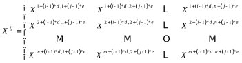 (2-1)
(2-1) ,
,  .
. (2-2)
(2-2) denotes the element in the weight vector w, p is the number of input matrix rows, q is the number of input matrix columns, and
  is the output feature map, whose dimensionality is related to the number of convolutional kernels, each of which is equipped with a unique set of initial weight matrices. For a single convolutional kernel, the dimension c of the resulting output feature map can be computed using the following equation:
  (2-3)
(2-3) (2-4)
(2-4)
 (2-6)
(2-6) (2-7)
(2-7) (2-8)
(2-8) (2-9)
(2-9) (2-10)
 is the new candidate cell state, wc and bc are the weights and bias terms of the input gate, respectively.
 (2-11)
 denotes the dot product.
 (2-12)
 (2-13)
 (2-14)
 (2-15)
 (2-16)
 represents the parameters of the discriminator. R and F are the number of true and false samples, respectively. yr denotes the labels of the true samples, yf denotes the labels of the generated samples, ar and af denote the labels of samples predicted by the sigmoid function, br and bf are the SoftMax function predicted sample categories.
 (2-17)
 (2-18)
 are the generator loss function and parameters.
 (2-19)
 (2-20)
 (2-21)
 represents the ratio of the number of positive and negative samples, S ranges from [0,1], and the better the model works, the closer the value of S is to 1.