<?xml version="1.0" encoding="UTF-8"?><!DOCTYPE article PUBLIC "-//NLM//DTD Journal Publishing DTD v3.0 20080202//EN" "http://dtd.nlm.nih.gov/publishing/3.0/journalpublishing3.dtd">
<article xmlns:mml="http://www.w3.org/1998/Math/MathML" xmlns:xlink="http://www.w3.org/1999/xlink" dtd-version="3.0" xml:lang="en" article-type="research article">
 <front>
  <journal-meta>
   <journal-id journal-id-type="publisher-id">
    jcc
   </journal-id>
   <journal-title-group>
    <journal-title>
     Journal of Computer and Communications
    </journal-title>
   </journal-title-group>
   <issn pub-type="epub">
    2327-5219
   </issn>
   <issn publication-format="print">
    2327-5227
   </issn>
   <publisher>
    <publisher-name>
     Scientific Research Publishing
    </publisher-name>
   </publisher>
  </journal-meta>
  <article-meta>
   <article-id pub-id-type="doi">
    10.4236/jcc.2024.1211004
   </article-id>
   <article-id pub-id-type="publisher-id">
    jcc-137286
   </article-id>
   <article-categories>
    <subj-group subj-group-type="heading">
     <subject>
      Articles
     </subject>
    </subj-group>
    <subj-group subj-group-type="Discipline-v2">
     <subject>
      Computer Science 
     </subject>
     <subject>
       Communications
     </subject>
    </subj-group>
   </article-categories>
   <title-group>
    Missing Data Imputation: A Comprehensive Review
   </title-group>
   <contrib-group>
    <contrib contrib-type="author" xlink:type="simple">
     <name name-style="western">
      <surname>
       Majed
      </surname>
      <given-names>
       Alwateer
      </given-names>
     </name> 
     <xref ref-type="aff" rid="aff1"> 
      <sup>1</sup>
     </xref>
    </contrib>
    <contrib contrib-type="author" xlink:type="simple">
     <name name-style="western">
      <surname>
       El-Sayed
      </surname>
      <given-names>
       Atlam
      </given-names>
     </name> 
     <xref ref-type="aff" rid="aff1"> 
      <sup>1</sup>
     </xref> 
     <xref ref-type="aff" rid="aff2"> 
      <sup>2</sup>
     </xref>
    </contrib>
    <contrib contrib-type="author" xlink:type="simple">
     <name name-style="western">
      <surname>
       Mahmoud Mohammed Abd
      </surname>
      <given-names>
       El-Raouf
      </given-names>
     </name> 
     <xref ref-type="aff" rid="aff3"> 
      <sup>3</sup>
     </xref>
    </contrib>
    <contrib contrib-type="author" xlink:type="simple">
     <name name-style="western">
      <surname>
       Osama A.
      </surname>
      <given-names>
       Ghoneim
      </given-names>
     </name> 
     <xref ref-type="aff" rid="aff4"> 
      <sup>4</sup>
     </xref>
    </contrib>
    <contrib contrib-type="author" xlink:type="simple">
     <name name-style="western">
      <surname>
       Ibrahim
      </surname>
      <given-names>
       Gad
      </given-names>
     </name> 
     <xref ref-type="aff" rid="aff2"> 
      <sup>2</sup>
     </xref>
    </contrib>
   </contrib-group> 
   <aff id="aff1">
    <addr-line>
     aDepartment of Computer Science, College of Computer Science and Engineering, Taibah University, Yanbu, Saudi Arabia
    </addr-line> 
   </aff> 
   <aff id="aff2">
    <addr-line>
     aComputer Science Department, Faculty of Science, Tanta University, Tanta, Egypt
    </addr-line> 
   </aff> 
   <aff id="aff3">
    <addr-line>
     aBasic and Applied Science Institute, College of Engineering and Technology, Arab Academy for Science and Technology (AAST), Alexandria, Egypt
    </addr-line> 
   </aff> 
   <aff id="aff4">
    <addr-line>
     aDepartment of Computer Science, Faculty of Computers and informatics, Tanta University, Tanta, Egypt
    </addr-line> 
   </aff> 
   <pub-date pub-type="epub">
    <day>
     31
    </day> 
    <month>
     10
    </month>
    <year>
     2024
    </year>
   </pub-date> 
   <volume>
    12
   </volume> 
   <issue>
    11
   </issue>
   <fpage>
    53
   </fpage>
   <lpage>
    75
   </lpage>
   <history>
    <date date-type="received">
     <day>
      25,
     </day>
     <month>
      September
     </month>
     <year>
      2024
     </year>
    </date>
    <date date-type="published">
     <day>
      8,
     </day>
     <month>
      September
     </month>
     <year>
      2024
     </year> 
    </date> 
    <date date-type="accepted">
     <day>
      8,
     </day>
     <month>
      November
     </month>
     <year>
      2024
     </year> 
    </date>
   </history>
   <permissions>
    <copyright-statement>
     © Copyright 2014 by authors and Scientific Research Publishing Inc. 
    </copyright-statement>
    <copyright-year>
     2014
    </copyright-year>
    <license>
     <license-p>
      This work is licensed under the Creative Commons Attribution International License (CC BY). http://creativecommons.org/licenses/by/4.0/
     </license-p>
    </license>
   </permissions>
   <abstract>
    Missing data presents a significant challenge in statistical analysis and machine learning, often resulting in biased outcomes and diminished efficiency. This comprehensive review investigates various imputation techniques, categorizing them into three primary approaches: deterministic methods, probabilistic models, and machine learning algorithms. Traditional techniques, including mean or mode imputation, regression imputation, and last observation carried forward, are evaluated alongside more contemporary methods such as multiple imputation, expectation-maximization, and deep learning strategies. The strengths and limitations of each approach are outlined. Key considerations for selecting appropriate methods, based on data characteristics and research objectives, are discussed. The importance of evaluating imputation’s impact on subsequent analyses is emphasized. This synthesis of recent advancements and best practices provides researchers with a robust framework for effectively handling missing data, thereby improving the reliability of empirical findings across diverse disciplines.
   </abstract>
   <kwd-group> 
    <kwd>
     Missing Data
    </kwd> 
    <kwd>
      Machine Learning
    </kwd> 
    <kwd>
      Prediction
    </kwd> 
    <kwd>
      Deep Learning
    </kwd> 
    <kwd>
      Imputation
    </kwd>
   </kwd-group>
  </article-meta>
 </front>
 <body>
  <sec id="s1">
   <title>1. Introduction</title>
   <p>Missing data can occur due to various reasons, such as participant non-response in surveys, equipment malfunction in experimental settings, or data entry errors <xref ref-type="bibr" rid="scirp.137286-1">
     [1]
    </xref> <xref ref-type="bibr" rid="scirp.137286-2">
     [2]
    </xref>. The presence of missing data can significantly impact statistical analyses and lead to incorrect conclusions if not properly addressed <xref ref-type="bibr" rid="scirp.137286-3">
     [3]
    </xref>. Missing data is a pervasive issue in empirical research across various disciplines, including social sciences, medical research, and data science <xref ref-type="bibr" rid="scirp.137286-4">
     [4]
    </xref>. It occurs when no value is available for a variable in an observation, potentially leading to incomplete datasets that can compromise the validity and reliability of statistical analyses <xref ref-type="bibr" rid="scirp.137286-5">
     [5]
    </xref> <xref ref-type="bibr" rid="scirp.137286-6">
     [6]
    </xref>.</p>
   <p>Missing values can significantly impact your analysis: They can introduce bias if not handled properly. Many machine learning algorithms can’t handle missing values that are out of the box. They can lead to the loss of important information if instances with missing values are simply discarded. Improperly handled missing values can lead to incorrect conclusions or predictions.</p>
   <p>Missing values can sneak into your data for a variety of reasons. Here are some common reasons: Data Entry Errors: Sometimes, it’s just human error. Someone might forget to input a value or accidentally delete one. Sensor Malfunctions: In IoT or scientific experiments, a faulty sensor might fail to record data at certain times <xref ref-type="bibr" rid="scirp.137286-7">
     [7]
    </xref>. Survey Non-Response: In surveys, respondents might skip questions they are uncomfortable answering or don’t understand. Merged Datasets: When combining data from multiple sources, some entries might not have corresponding values in all datasets. Data Corruption: During data transfer or storage, some values might get corrupted and become unreadable. Intentional Omissions: Some data might be intentionally left out due to privacy concerns or irrelevance. Sampling Issues: The data collection method might systematically miss certain types of data. Time-Sensitive Data: In time series data, values might be missing for periods when data wasn’t collected (e.g., weekends, holidays) <xref ref-type="bibr" rid="scirp.137286-8">
     [8]
    </xref>.</p>
   <p>Researchers typically encounter three main types of missing data mechanisms, as defined by Rubin <xref ref-type="bibr" rid="scirp.137286-4">
     [4]
    </xref>: 1) Missing Completely at Random (MCAR): The probability of missing data is unrelated to both observed and unobserved variables. 2) Missing at Random (MAR): The probability of missing data depends on observed variables but not on unobserved variables. 3) Missing Not at Random (MNAR): The probability of missing data depends on unobserved variables, including the missing data itself.</p>
   <p>Addressing missing data is of paramount importance in research for several reasons: 1) Bias reduction: Ignoring missing data or using simplistic methods like complete case analysis can lead to biased estimates and incorrect inferences <xref ref-type="bibr" rid="scirp.137286-9">
     [9]
    </xref>. Proper handling of missing data helps minimize this bias and improve the accuracy of research findings. 2) Statistical power: Missing data reduces the effective sample size, leading to decreased statistical power. Appropriate imputation techniques can help maintain or even increase power by utilizing all available information <xref ref-type="bibr" rid="scirp.137286-10">
     [10]
    </xref>. 3) Generalizability: Incomplete datasets may not be representative of the population of interest, potentially limiting the generalizability of research findings. Addressing missing data can help improve the external validity of results <xref ref-type="bibr" rid="scirp.137286-11">
     [11]
    </xref>. 4) Ethical considerations: In clinical trials and other human subjects research, ignoring missing data may lead to the waste of valuable data that participants have provided, raising ethical concerns. 5) Regulatory compliance: In some fields, such as clinical trials, regulatory bodies require proper handling and reporting of missing data <xref ref-type="bibr" rid="scirp.137286-12">
     [12]
    </xref>. 6) Improved decision-making: In applied settings, such as business analytics or public policy, accurate and complete data is essential for informed decision-making <xref ref-type="bibr" rid="scirp.137286-13">
     [13]
    </xref>.</p>
   <p>While imputation methods offer valuable tools for handling missing data, several challenges and considerations must be addressed to ensure effective and reliable results: 1) Handling different data types: Imputation methods must be able to handle various data types, including continuous, categorical, and mixed data <xref ref-type="bibr" rid="scirp.137286-14">
     [14]
    </xref>. 2) Dealing with high-dimensional data: As the number of variables increases, imputation becomes more challenging due to the curse of dimensionality <xref ref-type="bibr" rid="scirp.137286-15">
     [15]
    </xref>. 3) Computational efficiency: Some advanced imputation methods can be computationally intensive, necessitating efficient implementations for large-scale applications <xref ref-type="bibr" rid="scirp.137286-16">
     [16]
    </xref>. 4) Preserving data distributions and relationships: Imputation methods should maintain the statistical properties of the original data, including distributions and relationships between variables <xref ref-type="bibr" rid="scirp.137286-17">
     [17]
    </xref>.</p>
   <p>Missing data is a pervasive issue in research across various disciplines, often leading to biased or inefficient analyses <xref ref-type="bibr" rid="scirp.137286-4">
     [4]
    </xref>. Addressing missing data is crucial for maintaining the integrity and reliability of research findings <xref ref-type="bibr" rid="scirp.137286-18">
     [18]
    </xref>. This review aims to provide a comprehensive overview of missing data imputation techniques, their applications, and current challenges in the field.</p>
   <p>
    <xref ref-type="table" rid="table1">
     Table 1
    </xref> summarizing the recent papers on imputation methods published between 2017 and 2024, focusing on the year, model used, columns imputed, and key results.</p>
   <p>Given the critical nature of missing data in research, this comprehensive review aims to achieve the following objectives: 1) Provide an up-to-date synthesis of current missing data imputation techniques, including traditional methods and advanced machine learning approaches. 2) Critically evaluate the strengths and limitations of various imputation methods across different research contexts and data types. 3) Examine the impact of different missing data mechanisms on the performance of imputation techniques. 4) Explore emerging trends and future directions in missing data imputation, including the application of deep learning and artificial intelligence techniques.</p>
   <p>Offer practical guidelines to help researchers select appropriate imputation methods based on their specific research context, data characteristics, and analysis goals. Identify gaps in the current literature and propose areas for future research in missing data imputation.</p>
   <p>By addressing these objectives, this review aims to provide researchers, statisticians, and data scientists with a comprehensive understanding of missing data imputation techniques, their applications, and their implications for research integrity and validity.</p>
   <table-wrap id="table1">
    <label>
     <xref ref-type="table" rid="table1">
      Table 1
     </xref></label>
    <caption>
     <title>
      <xref ref-type="bibr" rid="scirp.137286-"></xref>Table 1. Summary of imputation methods in published papers (2017-2024).</title>
    </caption>
    <table class="MsoTableGrid custom-table" border="0" cellspacing="0" cellpadding="0"> 
     <tr> 
      <td class="custom-bottom-td acenter" width="16.39%"><p style="text-align:center">Paper title</p></td> 
      <td class="custom-bottom-td acenter" width="8.74%"><p style="text-align:center">Year</p></td> 
      <td class="custom-bottom-td acenter" width="19.23%"><p style="text-align:center">Model used</p></td> 
      <td class="custom-bottom-td acenter" width="19.24%"><p style="text-align:center">Columns imputed</p></td> 
      <td class="custom-bottom-td acenter" width="36.39%"><p style="text-align:center">Key results</p></td> 
     </tr> 
     <tr> 
      <td class="custom-top-td acenter" width="16.39%"><p style="text-align:center">Doreswamy et al. <xref ref-type="bibr" rid="scirp.137286-19">
         [19]
        </xref></p></td> 
      <td class="custom-top-td acenter" width="8.74%"><p style="text-align:center">2017</p></td> 
      <td class="custom-top-td acenter" width="19.23%"><p style="text-align:center">kernel ridge, linear regression, random forest, SVM, and KNN</p></td> 
      <td class="custom-top-td acenter" width="19.24%"><p style="text-align:center">Multiple variables of NCDC weather dataset</p></td> 
      <td class="custom-top-td acenter" width="36.39%"><p style="text-align:center">Accounted for temporal dependencies in longitudinal data, leading to more accurate estimates of parameters and improved model performance.</p></td> 
     </tr> 
     <tr> 
      <td class="acenter" width="16.39%"><p style="text-align:center">Hosahalli et al. <xref ref-type="bibr" rid="scirp.137286-20">
         [20]
        </xref></p></td> 
      <td class="acenter" width="8.74%"><p style="text-align:center">2018</p></td> 
      <td class="acenter" width="19.23%"><p style="text-align:center">Machine learning models</p></td> 
      <td class="acenter" width="19.24%"><p style="text-align:center">NCDC weather datasets</p></td> 
      <td class="acenter" width="36.39%"><p style="text-align:center">Improved accuracy of predictive models for NCDC weather dataset compared to single imputation methods.</p></td> 
     </tr> 
     <tr> 
      <td class="acenter" width="16.39%"><p style="text-align:center">Khanani <xref ref-type="bibr" rid="scirp.137286-21">
         [21]
        </xref></p></td> 
      <td class="acenter" width="8.74%"><p style="text-align:center">2021</p></td> 
      <td class="acenter" width="19.23%"><p style="text-align:center">Predictive mean matching (PMM)</p></td> 
      <td class="acenter" width="19.24%"><p style="text-align:center">Education data</p></td> 
      <td class="acenter" width="36.39%"><p style="text-align:center">Demonstrated effectiveness in imputing missing values in educational data from a public school with both numerical and categorical features.</p></td> 
     </tr> 
     <tr> 
      <td class="acenter" width="16.39%"><p style="text-align:center">Thakur et al. <xref ref-type="bibr" rid="scirp.137286-22">
         [22]
        </xref></p></td> 
      <td class="acenter" width="8.74%"><p style="text-align:center">2021</p></td> 
      <td class="acenter" width="19.23%"><p style="text-align:center">Machine learning</p></td> 
      <td class="acenter" width="19.24%"><p style="text-align:center">Time series data</p></td> 
      <td class="acenter" width="36.39%"><p style="text-align:center">Provided a comprehensive overview of multiple imputation techniques and their applications in machine learning, highlighting their advantages and limitations.</p></td> 
     </tr> 
     <tr> 
      <td class="acenter" width="16.39%"><p style="text-align:center">Psychogyios et al. <xref ref-type="bibr" rid="scirp.137286-23">
         [23]
        </xref></p></td> 
      <td class="acenter" width="8.74%"><p style="text-align:center">2023</p></td> 
      <td class="acenter" width="19.23%"><p style="text-align:center">KNN-MICE-GAN</p></td> 
      <td class="acenter" width="19.24%"><p style="text-align:center">Age, gender, diagnosis codes, lab results</p></td> 
      <td class="acenter" width="36.39%"><p style="text-align:center">Improved accuracy of predictive models for hospital readmission compared to single imputation methods.</p></td> 
     </tr> 
     <tr> 
      <td class="acenter" width="16.39%"><p style="text-align:center">Omar et al. <xref ref-type="bibr" rid="scirp.137286-24">
         [24]
        </xref></p></td> 
      <td class="acenter" width="8.74%"><p style="text-align:center">2023</p></td> 
      <td class="acenter" width="19.23%"><p style="text-align:center">Random forest, decision tree, neural network and support vector machine</p></td> 
      <td class="acenter" width="19.24%"><p style="text-align:center">Dropout in higher education</p></td> 
      <td class="acenter" width="36.39%"><p style="text-align:center">The results showed that the Random Forest algorithm obtained the best performance, with an AUC of 0.9623 in the prediction of college dropout.</p></td> 
     </tr> 
     <tr> 
      <td class="acenter" width="16.39%"><p style="text-align:center">Nida et al. <xref ref-type="bibr" rid="scirp.137286-25">
         [25]
        </xref></p></td> 
      <td class="acenter" width="8.74%"><p style="text-align:center">2023</p></td> 
      <td class="acenter" width="19.23%"><p style="text-align:center">Mean imputation, KNN, PMM</p></td> 
      <td class="acenter" width="19.24%"><p style="text-align:center">Rainfall data</p></td> 
      <td class="acenter" width="36.39%"><p style="text-align:center">The KNN achieved high imputation accuracy for missing rainfall variables values, improving the analysis of complex weather datasets.</p></td> 
     </tr> 
     <tr> 
      <td class="acenter" width="16.39%"><p style="text-align:center">Psychogyios et al. <xref ref-type="bibr" rid="scirp.137286-23">
         [23]
        </xref></p></td> 
      <td class="acenter" width="8.74%"><p style="text-align:center">2023</p></td> 
      <td class="acenter" width="19.23%"><p style="text-align:center">GAN</p></td> 
      <td class="acenter" width="19.24%"><p style="text-align:center">Electronic health records</p></td> 
      <td class="acenter" width="36.39%"><p style="text-align:center">The results show that GAN achieved high imputation accuracy and outperform the standard baselines.</p></td> 
     </tr> 
     <tr> 
      <td class="acenter" width="16.39%"><p style="text-align:center">Teegavarapu et al. <xref ref-type="bibr" rid="scirp.137286-26">
         [26]
        </xref></p></td> 
      <td class="acenter" width="8.74%"><p style="text-align:center">2024</p></td> 
      <td class="acenter" width="19.23%"><p style="text-align:center">Spatial and temporal interpolation methods</p></td> 
      <td class="acenter" width="19.24%"><p style="text-align:center">Hydrometeorological data</p></td> 
      <td class="acenter" width="36.39%"><p style="text-align:center">Provided a comprehensive overview of multiple imputation techniques for precipitation, temperature, and streamflows and highlighting their advantages and limitations.</p></td> 
     </tr> 
     <tr> 
      <td class="acenter" width="16.39%"><p style="text-align:center">Almeida et al. <xref ref-type="bibr" rid="scirp.137286-27">
         [27]
        </xref></p></td> 
      <td class="acenter" width="8.74%"><p style="text-align:center">2024</p></td> 
      <td class="acenter" width="19.23%"><p style="text-align:center">Focalize K-NN method</p></td> 
      <td class="acenter" width="19.24%"><p style="text-align:center">Time series data</p></td> 
      <td class="acenter" width="36.39%"><p style="text-align:center">The results demonstrated that the effectiveness of Focalize K-NN for imputing missing values in time series data.</p></td> 
     </tr> 
     <tr> 
      <td class="acenter" width="16.39%"><p style="text-align:center">Kowsar et al. <xref ref-type="bibr" rid="scirp.137286-28">
         [28]
        </xref></p></td> 
      <td class="acenter" width="8.74%"><p style="text-align:center">2024</p></td> 
      <td class="acenter" width="19.23%"><p style="text-align:center">Self-attention imputation method</p></td> 
      <td class="acenter" width="19.24%"><p style="text-align:center">Electronic health records</p></td> 
      <td class="acenter" width="36.39%"><p style="text-align:center">The proposed imputation method demonstrates superior performance across a range of missing data proportions (10% to 50%) under the assumption of missing completely at random (MCAR).</p></td> 
     </tr> 
    </table>
   </table-wrap>
  </sec><sec id="s2">
   <title>
    <xref ref-type="bibr" rid="scirp.137286-"></xref>2. Missing Data Types</title>
   <p>Understanding the mechanisms of missingness is essential for selecting appropriate imputation methods and accurately interpreting results. Rubin’s classification system for missing data, which remains fundamental to the field, identifies three main types of missing data <xref ref-type="bibr" rid="scirp.137286-18">
     [18]
    </xref>.</p>
   <sec id="s2_1">
    <title>
     <xref ref-type="bibr" rid="scirp.137286-"></xref>2.1. Missing Completely at Random (MCAR)</title>
    <p>Missingness is considered completely random when it does not depend on any other variables. This condition, known as Missing Completely at Random (MCAR), occurs when the probability of missing data is unrelated to both observed and unobserved variables <xref ref-type="bibr" rid="scirp.137286-29">
      [29]
     </xref>-<xref ref-type="bibr" rid="scirp.137286-31">
      [31]
     </xref>. In this scenario, the missingness is purely due to chance, with no influence from any characteristics of the data <xref ref-type="bibr" rid="scirp.137286-4">
      [4]
     </xref>. MCAR is the most stringent assumption and rarely occurs in practice. However, when data are MCAR, analyses using only complete cases will be unbiased, although potentially inefficient <xref ref-type="bibr" rid="scirp.137286-1">
      [1]
     </xref>.</p>
    <p>Let 
     <math xmlns="http://www.w3.org/1998/Math/MathML"> <mi>
        R 
      </mi> 
     </math> be the missingness indicator and 
     <math xmlns="http://www.w3.org/1998/Math/MathML"> <mi>
        Y 
      </mi> 
     </math> be the complete data. MCAR can be defined as: 
     <math xmlns="http://www.w3.org/1998/Math/MathML"> <mrow> 
       <mi>
         P 
       </mi> 
       <mrow> 
        <mo>
          ( 
        </mo> 
        <mrow> 
         <mi>
           R 
         </mi> 
         <mo>
           | 
         </mo> 
         <mi>
           Y 
         </mi> 
        </mrow> 
        <mo>
          ) 
        </mo> 
       </mrow> 
       <mo>
         = 
       </mo> 
       <mi>
         P 
       </mi> 
       <mrow> 
        <mo>
          ( 
        </mo> 
        <mi>
          R 
        </mi> 
        <mo>
          ) 
        </mo> 
       </mrow> 
      </mrow> 
     </math>.</p>
    <p>For example, in a survey, some participants accidentally skip questions regardless of their characteristics or responses to other items.</p>
   </sec>
   <sec id="s2_2">
    <title>
     <xref ref-type="bibr" rid="scirp.137286-"></xref>2.2. Missing at Random (MAR)</title>
    <p>The probability of missing data depends on other observed variables but not on the missing data itself. This condition, known as Missing at Random (MAR), occurs when the likelihood of missingness is related to observed variables but not to unobserved ones <xref ref-type="bibr" rid="scirp.137286-18">
      [18]
     </xref>. MAR represents a less stringent assumption compared to Missing Completely at Random (MCAR) and is often more realistic in practice. In summary, data are considered MAR when the probability of missingness is influenced by observed variables while remaining independent of unobserved variables <xref ref-type="bibr" rid="scirp.137286-18">
      [18]
     </xref>. MAR allows for relationships between observed variables and the probability of missingness. Many modern imputation methods, such as multiple imputation, assume MAR <xref ref-type="bibr" rid="scirp.137286-17">
      [17]
     </xref>.</p>
    <p>Let 
     <math xmlns="http://www.w3.org/1998/Math/MathML"> <mrow> 
       <msub> 
        <mi>
          Y 
        </mi> 
        <mrow> 
         <mi>
           o 
         </mi> 
         <mi>
           b 
         </mi> 
         <mi>
           s 
         </mi> 
        </mrow> 
       </msub> 
      </mrow> 
     </math> be the observed data and 
     <math xmlns="http://www.w3.org/1998/Math/MathML"> <mrow> 
       <msub> 
        <mi>
          Y 
        </mi> 
        <mrow> 
         <mi>
           m 
         </mi> 
         <mi>
           i 
         </mi> 
         <mi>
           s 
         </mi> 
        </mrow> 
       </msub> 
      </mrow> 
     </math> be the missing data. MAR can be defined as: 
     <math xmlns="http://www.w3.org/1998/Math/MathML"> <mrow> 
       <mi>
         P 
       </mi> 
       <mrow> 
        <mo>
          ( 
        </mo> 
        <mrow> 
         <mi>
           R 
         </mi> 
         <mo>
           | 
         </mo> 
         <mi>
           Y 
         </mi> 
        </mrow> 
        <mo>
          ) 
        </mo> 
       </mrow> 
       <mo>
         = 
       </mo> 
       <mi>
         P 
       </mi> 
       <mrow> 
        <mo>
          ( 
        </mo> 
        <mrow> 
         <mi>
           R 
         </mi> 
         <mo>
           | 
         </mo> 
         <msub> 
          <mi>
            Y 
          </mi> 
          <mrow> 
           <mi>
             o 
           </mi> 
           <mi>
             b 
           </mi> 
           <mi>
             s 
           </mi> 
          </mrow> 
         </msub> 
        </mrow> 
        <mo>
          ) 
        </mo> 
       </mrow> 
      </mrow> 
     </math>.</p>
    <p>For example, in a longitudinal study on income, older participants are more likely to withhold information about their earnings, but this likelihood is not related to the actual income amount after accounting for age. For example, men might be less likely to answer questions about emotions in a survey.</p>
   </sec>
   <sec id="s2_3">
    <title>
     <xref ref-type="bibr" rid="scirp.137286-"></xref>2.3. Missing Not at Random (MNAR)</title>
    <p>Missingness is categorized as Missing Not at Random (MNAR) when the probability of missing data is influenced by the values of the missing data itself or by unobserved variables. In this case, the missingness is directly related to the unobserved values <xref ref-type="bibr" rid="scirp.137286-4">
      [4]
     </xref>. MNAR is the most challenging type of missing data to handle. Standard imputation methods can yield biased results, necessitating specialized techniques or sensitivity analyses to address the issue effectively <xref ref-type="bibr" rid="scirp.137286-32">
      [32]
     </xref>.</p>
    <p>MNAR occurs when the probability of missing data depends on unobserved variables or the missing values themselves <xref ref-type="bibr" rid="scirp.137286-4">
      [4]
     </xref>. This is the most challenging type of missingness to address and often requires specialized techniques. MNAR occurs when: 
     <math xmlns="http://www.w3.org/1998/Math/MathML"> <mrow> 
       <mi>
         P 
       </mi> 
       <mrow> 
        <mo>
          ( 
        </mo> 
        <mrow> 
         <mi>
           R 
         </mi> 
         <mo>
           | 
         </mo> 
         <mi>
           Y 
         </mi> 
        </mrow> 
        <mo>
          ) 
        </mo> 
       </mrow> 
       <mo>
         ≠ 
       </mo> 
       <mi>
         P 
       </mi> 
       <mrow> 
        <mo>
          ( 
        </mo> 
        <mrow> 
         <mi>
           R 
         </mi> 
         <mo>
           | 
         </mo> 
         <msub> 
          <mi>
            Y 
          </mi> 
          <mrow> 
           <mi>
             o 
           </mi> 
           <mi>
             b 
           </mi> 
           <mi>
             s 
           </mi> 
          </mrow> 
         </msub> 
        </mrow> 
        <mo>
          ) 
        </mo> 
       </mrow> 
      </mrow> 
     </math>.</p>
    <p>An example of MNAR is in a mental health survey, participants with severe depression may be less likely to complete questions about their symptoms, with this likelihood directly related to the severity of their undisclosed condition. Similarly, individuals with high incomes might be less inclined to report their income in a survey.</p>
    <p>In practice, it is often impossible to definitively determine whether data are MAR or MNAR based solely on observed data <xref ref-type="bibr" rid="scirp.137286-33">
      [33]
     </xref>. Therefore, researchers often must rely on subject-matter knowledge and conduct sensitivity analyses to assess the robustness of their findings under different missing data assumptions <xref ref-type="bibr" rid="scirp.137286-17">
      [17]
     </xref>.</p>
   </sec>
  </sec><sec id="s3">
   <title>
    <xref ref-type="bibr" rid="scirp.137286-"></xref>3. Missing Value Imputation</title>
   <fig id="fig1" position="float">
    <label>Figure 1</label>
    <caption>
     <title>Figure 1. The flowchart of imputation of missing values.</title>
    </caption>
    <graphic mimetype="image" position="float" xlink:type="simple" xlink:href="https://html.scirp.org/file/1732927-rId29.jpeg?20241111023631" />
   </fig>
   <p>The problem of missing data imputation arises when a dataset contains unobserved values for certain features. Let 
    <math xmlns="http://www.w3.org/1998/Math/MathML"> <mrow> 
      <mi>
        X 
      </mi> 
      <mo>
        = 
      </mo> 
      <mrow> 
       <mo>
         ( 
       </mo> 
       <mrow> 
        <msub> 
         <mi>
           X 
         </mi> 
         <mn>
           1 
         </mn> 
        </msub> 
        <mo>
          , 
        </mo> 
        <msub> 
         <mi>
           X 
         </mi> 
         <mn>
           2 
         </mn> 
        </msub> 
        <mo>
          , 
        </mo> 
        <mo>
          ⋯ 
        </mo> 
        <mo>
          , 
        </mo> 
        <msub> 
         <mi>
           X 
         </mi> 
         <mi>
           n 
         </mi> 
        </msub> 
       </mrow> 
       <mo>
         ) 
       </mo> 
      </mrow> 
      <mo>
        ∈ 
      </mo> 
      <msup> 
       <mi>
         ℝ 
       </mi> 
       <mi>
         n 
       </mi> 
      </msup> 
     </mrow> 
    </math> represent a random vector, where each 
    <math xmlns="http://www.w3.org/1998/Math/MathML"> <mrow> 
      <msub> 
       <mi>
         X 
       </mi> 
       <mi>
         i 
       </mi> 
      </msub> 
     </mrow> 
    </math> corresponds to a feature and follows a distribution 
    <math xmlns="http://www.w3.org/1998/Math/MathML"> <mrow> 
      <mi>
        P 
      </mi> 
      <mrow> 
       <mo>
         ( 
       </mo> 
       <mi>
         X 
       </mi> 
       <mo>
         ) 
       </mo> 
      </mrow> 
     </mrow> 
    </math>. A binary mask vector 
    <math xmlns="http://www.w3.org/1998/Math/MathML"> <mrow> 
      <mi>
        M 
      </mi> 
      <mo>
        = 
      </mo> 
      <mrow> 
       <mo>
         ( 
       </mo> 
       <mrow> 
        <msub> 
         <mi>
           M 
         </mi> 
         <mn>
           1 
         </mn> 
        </msub> 
        <mo>
          , 
        </mo> 
        <msub> 
         <mi>
           M 
         </mi> 
         <mn>
           2 
         </mn> 
        </msub> 
        <mo>
          , 
        </mo> 
        <mo>
          ⋯ 
        </mo> 
        <mo>
          , 
        </mo> 
        <msub> 
         <mi>
           M 
         </mi> 
         <mi>
           n 
         </mi> 
        </msub> 
       </mrow> 
       <mo>
         ) 
       </mo> 
      </mrow> 
     </mrow> 
    </math> indicates the presence or absence of observations, with 
    <math xmlns="http://www.w3.org/1998/Math/MathML"> <mrow> 
      <msub> 
       <mi>
         M 
       </mi> 
       <mi>
         i 
       </mi> 
      </msub> 
      <mo>
        = 
      </mo> 
      <mn>
        1 
      </mn> 
     </mrow> 
    </math> denoting an observed value and 
    <math xmlns="http://www.w3.org/1998/Math/MathML"> <mrow> 
      <msub> 
       <mi>
         M 
       </mi> 
       <mi>
         i 
       </mi> 
      </msub> 
      <mo>
        = 
      </mo> 
      <mn>
        0 
      </mn> 
     </mrow> 
    </math> a missing value. Given a dataset of 
    <math xmlns="http://www.w3.org/1998/Math/MathML"> <mi>
       d 
     </mi> 
    </math> instances 
    <math xmlns="http://www.w3.org/1998/Math/MathML"> <mrow> 
      <msub> 
       <mrow> 
        <mrow> 
         <mo>
           { 
         </mo> 
         <mrow> 
          <mrow> 
           <mo>
             ( 
           </mo> 
           <mrow> 
            <msub> 
             <mi>
               X 
             </mi> 
             <mi>
               i 
             </mi> 
            </msub> 
            <mo>
              , 
            </mo> 
            <msub> 
             <mi>
               M 
             </mi> 
             <mi>
               i 
             </mi> 
            </msub> 
           </mrow> 
           <mo>
             ) 
           </mo> 
          </mrow> 
         </mrow> 
         <mo>
           } 
         </mo> 
        </mrow> 
       </mrow> 
       <mrow> 
        <mi>
          i 
        </mi> 
        <mo>
          = 
        </mo> 
        <mn>
          0 
        </mn> 
        <mo>
          , 
        </mo> 
        <mo>
          ⋯ 
        </mo> 
        <mo>
          , 
        </mo> 
        <mi>
          d 
        </mi> 
        <mo>
          − 
        </mo> 
        <mn>
          1 
        </mn> 
       </mrow> 
      </msub> 
     </mrow> 
    </math>, an imputed dataset is constructed by replacing missing values (where 
    <math xmlns="http://www.w3.org/1998/Math/MathML"> <mrow> 
      <msub> 
       <mi>
         M 
       </mi> 
       <mrow> 
        <mi>
          i 
        </mi> 
        <mi>
          j 
        </mi> 
       </mrow> 
      </msub> 
      <mo>
        = 
      </mo> 
      <mn>
        0 
      </mn> 
     </mrow> 
    </math>) in the observed data 
    <math xmlns="http://www.w3.org/1998/Math/MathML"> <mrow> 
      <msub> 
       <mi>
         X 
       </mi> 
       <mi>
         i 
       </mi> 
      </msub> 
     </mrow> 
    </math> with pre-imputed values, potentially random noise, resulting in 
    <math xmlns="http://www.w3.org/1998/Math/MathML"> <mrow> 
      <msub> 
       <mover accent="true"> 
        <mi>
          X 
        </mi> 
        <mo>
          ^ 
        </mo> 
       </mover> 
       <mi>
         i 
       </mi> 
      </msub> 
     </mrow> 
    </math>. The objective is to develop an imputation model, IMP, that generates an imputed dataset 
    <math xmlns="http://www.w3.org/1998/Math/MathML"> <mrow> 
      <msub> 
       <mrow> 
        <mrow> 
         <mo>
           { 
         </mo> 
         <mrow> 
          <msub> 
           <mover accent="true"> 
            <mi>
              X 
            </mi> 
            <mo>
              ˜ 
            </mo> 
           </mover> 
           <mi>
             i 
           </mi> 
          </msub> 
          <mo>
            = 
          </mo> 
          <mi>
            I 
          </mi> 
          <mi>
            M 
          </mi> 
          <mi>
            P 
          </mi> 
          <mrow> 
           <mo>
             ( 
           </mo> 
           <mrow> 
            <msub> 
             <mover accent="true"> 
              <mi>
                X 
              </mi> 
              <mo>
                ^ 
              </mo> 
             </mover> 
             <mi>
               i 
             </mi> 
            </msub> 
            <mo>
              , 
            </mo> 
            <msub> 
             <mi>
               M 
             </mi> 
             <mi>
               i 
             </mi> 
            </msub> 
           </mrow> 
           <mo>
             ) 
           </mo> 
          </mrow> 
         </mrow> 
         <mo>
           } 
         </mo> 
        </mrow> 
       </mrow> 
       <mrow> 
        <mi>
          i 
        </mi> 
        <mo>
          = 
        </mo> 
        <mn>
          0 
        </mn> 
        <mo>
          , 
        </mo> 
        <mo>
          ⋯ 
        </mo> 
        <mo>
          , 
        </mo> 
        <mi>
          d 
        </mi> 
        <mo>
          − 
        </mo> 
        <mn>
          1 
        </mn> 
       </mrow> 
      </msub> 
     </mrow> 
    </math> such that each imputed sample 
    <math xmlns="http://www.w3.org/1998/Math/MathML"> <mrow> 
      <msub> 
       <mover accent="true"> 
        <mi>
          X 
        </mi> 
        <mo>
          ˜ 
        </mo> 
       </mover> 
       <mi>
         i 
       </mi> 
      </msub> 
     </mrow> 
    </math> is drawn from the conditional distribution 
    <math xmlns="http://www.w3.org/1998/Math/MathML"> <mrow> 
      <mi>
        P 
      </mi> 
      <mo stretchy="false">
        ( 
      </mo> 
      <mi>
        X 
      </mi> 
      <mo>
        | 
      </mo> 
      <msub> 
       <mover accent="true"> 
        <mi>
          X 
        </mi> 
        <mo>
          ˜ 
        </mo> 
       </mover> 
       <mi>
         i 
       </mi> 
      </msub> 
      <mo stretchy="false">
        ) 
      </mo> 
     </mrow> 
    </math>, thereby preserving the original data’s distributional properties. This yields a complete dataset 
    <math xmlns="http://www.w3.org/1998/Math/MathML"> <mover accent="true"> 
      <mi>
        X 
      </mi> 
      <mo>
        ¯ 
      </mo> 
     </mover> 
    </math>, where 
    <math xmlns="http://www.w3.org/1998/Math/MathML"> <mrow> 
      <msub> 
       <mover accent="true"> 
        <mi>
          X 
        </mi> 
        <mo>
          ¯ 
        </mo> 
       </mover> 
       <mi>
         i 
       </mi> 
      </msub> 
      <mo>
        = 
      </mo> 
      <msub> 
       <mi>
         X 
       </mi> 
       <mi>
         i 
       </mi> 
      </msub> 
      <mo>
        ⊙ 
      </mo> 
      <msub> 
       <mi>
         M 
       </mi> 
       <mi>
         i 
       </mi> 
      </msub> 
      <mo>
        + 
      </mo> 
      <mrow> 
       <mo>
         ( 
       </mo> 
       <mrow> 
        <mn>
          1 
        </mn> 
        <mo>
          − 
        </mo> 
        <msub> 
         <mi>
           M 
         </mi> 
         <mi>
           i 
         </mi> 
        </msub> 
       </mrow> 
       <mo>
         ) 
       </mo> 
      </mrow> 
      <mo>
        ⊙ 
      </mo> 
      <msub> 
       <mover accent="true"> 
        <mi>
          X 
        </mi> 
        <mo>
          ˜ 
        </mo> 
       </mover> 
       <mi>
         i 
       </mi> 
      </msub> 
     </mrow> 
    </math> for each sample 
    <math xmlns="http://www.w3.org/1998/Math/MathML"> <mi>
       i 
     </mi> 
    </math>.</p>
   <p>Following imputation of missing values, predictive modeling was performed as shown in <xref ref-type="fig" rid="fig1">
     Figure 1
    </xref>. Application of 
    <math xmlns="http://www.w3.org/1998/Math/MathML"> <mi>
       S 
     </mi> 
    </math> distinct imputation algorithms, 
    <math xmlns="http://www.w3.org/1998/Math/MathML"> <mrow> 
      <msub> 
       <mi>
         A 
       </mi> 
       <mn>
         0 
       </mn> 
      </msub> 
      <mo>
        , 
      </mo> 
      <msub> 
       <mi>
         A 
       </mi> 
       <mn>
         1 
       </mn> 
      </msub> 
      <mo>
        , 
      </mo> 
      <mo>
        ⋯ 
      </mo> 
      <mo>
        , 
      </mo> 
      <msub> 
       <mi>
         A 
       </mi> 
       <mrow> 
        <mi>
          S 
        </mi> 
        <mo>
          − 
        </mo> 
        <mn>
          1 
        </mn> 
       </mrow> 
      </msub> 
     </mrow> 
    </math>, to the original dataset 
    <math xmlns="http://www.w3.org/1998/Math/MathML"> <mi>
       X 
     </mi> 
    </math> yielded 
    <math xmlns="http://www.w3.org/1998/Math/MathML"> <mi>
       S 
     </mi> 
    </math> completed datasets, denoted 
    <math xmlns="http://www.w3.org/1998/Math/MathML"> <mrow> 
      <msub> 
       <mover accent="true"> 
        <mi>
          D 
        </mi> 
        <mo>
          ¯ 
        </mo> 
       </mover> 
       <mn>
         1 
       </mn> 
      </msub> 
      <mo>
        , 
      </mo> 
      <msub> 
       <mover accent="true"> 
        <mi>
          D 
        </mi> 
        <mo>
          ¯ 
        </mo> 
       </mover> 
       <mn>
         2 
       </mn> 
      </msub> 
      <mo>
        , 
      </mo> 
      <mo>
        ⋯ 
      </mo> 
      <mo>
        , 
      </mo> 
      <msub> 
       <mover accent="true"> 
        <mi>
          D 
        </mi> 
        <mo>
          ¯ 
        </mo> 
       </mover> 
       <mi>
         S 
       </mi> 
      </msub> 
     </mrow> 
    </math>. A standard predictive model, 
    <math xmlns="http://www.w3.org/1998/Math/MathML"> <mi>
       P 
     </mi> 
    </math>, was then applied to each of these completed datasets to predict the outcome.</p>
  </sec><sec id="s4">
   <title>
    <xref ref-type="bibr" rid="scirp.137286-"></xref>4. Methods</title>
   <p>This study evaluated several imputation methods for handling missing data, ranging from simple statistical techniques to more sophisticated deep learning approaches. Specific methods included.</p>
   <sec id="s4_1">
    <title>
     <xref ref-type="bibr" rid="scirp.137286-"></xref>4.1. Traditional Imputation Methods</title>
    <p>Traditional methods for handling missing data have been widely used due to their simplicity and ease of implementation <xref ref-type="bibr" rid="scirp.137286-1">
      [1]
     </xref>. Traditional imputation methods are widely used to handle missing data in datasets. These methods aim to replace missing values with plausible estimates based on the available data. The most common traditional imputation techniques are discussed as follows.</p>
    <p>Missing categorical values were replaced with the mode, while missing numerical values were replaced with the mean of the corresponding feature. This method involves replacing missing values with the mean or median of the observed values for that variable <xref ref-type="bibr" rid="scirp.137286-4">
      [4]
     </xref>. Although simple, this approach can result in biased estimates and an underestimation of standard errors. For numerical data, missing values are replaced with the mean or median of the non-missing values in the same column, while for categorical data, the mode (most frequent value) is utilized.</p>
    <p>This iterative approach uses mean/mode imputation to initialize the dataset <xref ref-type="bibr" rid="scirp.137286-16">
      [16]
     </xref>. Then, a random forest is trained to predict the missing values in each feature, iteratively refining the imputed values until convergence (defined by a lack of improvement in the imputed matrix). Convergence criteria included a maximum of 20 iterations and 100 trees. The difference between successive imputed matrices ( 
     <math xmlns="http://www.w3.org/1998/Math/MathML"> <mrow> 
       <msub> 
        <mi>
          M 
        </mi> 
        <mrow> 
         <mi>
           i 
         </mi> 
         <mi>
           m 
         </mi> 
         <mi>
           p 
         </mi> 
         <mo>
           _ 
         </mo> 
         <mi>
           n 
         </mi> 
         <mi>
           e 
         </mi> 
         <mi>
           w 
         </mi> 
        </mrow> 
       </msub> 
      </mrow> 
     </math> and 
     <math xmlns="http://www.w3.org/1998/Math/MathML"> <mrow> 
       <msub> 
        <mi>
          M 
        </mi> 
        <mrow> 
         <mi>
           i 
         </mi> 
         <mi>
           m 
         </mi> 
         <mi>
           p 
         </mi> 
         <mo>
           _ 
         </mo> 
         <mi>
           o 
         </mi> 
         <mi>
           l 
         </mi> 
         <mi>
           d 
         </mi> 
        </mrow> 
       </msub> 
      </mrow> 
     </math>) for numerical ( 
     <math xmlns="http://www.w3.org/1998/Math/MathML"> <mi>
        N 
      </mi> 
     </math>) and categorical ( 
     <math xmlns="http://www.w3.org/1998/Math/MathML"> <mi>
        F 
      </mi> 
     </math>) features was measured as:</p>
    <p>
     <math xmlns="http://www.w3.org/1998/Math/MathML"> <mrow> 
       <msub> 
        <mi>
          δ 
        </mi> 
        <mi>
          N 
        </mi> 
       </msub> 
       <mo>
         = 
       </mo> 
       <mfrac> 
        <mrow> 
         <msub> 
          <mstyle mathsize="140%" displaystyle="true"> 
           <mo>
             ∑ 
           </mo> 
          </mstyle> 
          <mrow> 
           <mi>
             j 
           </mi> 
           <mo>
             ∈ 
           </mo> 
           <mi>
             N 
           </mi> 
          </mrow> 
         </msub> 
         <msup> 
          <mrow> 
           <mrow> 
            <mo>
              ( 
            </mo> 
            <mrow> 
             <msubsup> 
              <mi>
                M 
              </mi> 
              <mrow> 
               <mi>
                 n 
               </mi> 
               <mi>
                 e 
               </mi> 
               <mi>
                 w 
               </mi> 
              </mrow> 
              <mrow> 
               <mi>
                 i 
               </mi> 
               <mi>
                 m 
               </mi> 
               <mi>
                 p 
               </mi> 
              </mrow> 
             </msubsup> 
             <mo>
               − 
             </mo> 
             <msubsup> 
              <mi>
                M 
              </mi> 
              <mrow> 
               <mi>
                 o 
               </mi> 
               <mi>
                 l 
               </mi> 
               <mi>
                 d 
               </mi> 
              </mrow> 
              <mrow> 
               <mi>
                 i 
               </mi> 
               <mi>
                 m 
               </mi> 
               <mi>
                 p 
               </mi> 
              </mrow> 
             </msubsup> 
            </mrow> 
            <mo>
              ) 
            </mo> 
           </mrow> 
          </mrow> 
          <mn>
            2 
          </mn> 
         </msup> 
        </mrow> 
        <mrow> 
         <msub> 
          <mstyle mathsize="140%" displaystyle="true"> 
           <mo>
             ∑ 
           </mo> 
          </mstyle> 
          <mrow> 
           <mi>
             j 
           </mi> 
           <mo>
             ∈ 
           </mo> 
           <mi>
             N 
           </mi> 
          </mrow> 
         </msub> 
         <msup> 
          <mrow> 
           <mrow> 
            <mo>
              ( 
            </mo> 
            <mrow> 
             <msubsup> 
              <mi>
                M 
              </mi> 
              <mrow> 
               <mi>
                 n 
               </mi> 
               <mi>
                 e 
               </mi> 
               <mi>
                 w 
               </mi> 
              </mrow> 
              <mrow> 
               <mi>
                 i 
               </mi> 
               <mi>
                 m 
               </mi> 
               <mi>
                 p 
               </mi> 
              </mrow> 
             </msubsup> 
            </mrow> 
            <mo>
              ) 
            </mo> 
           </mrow> 
          </mrow> 
          <mn>
            2 
          </mn> 
         </msup> 
        </mrow> 
       </mfrac> 
      </mrow> 
     </math> (1)</p>
    <p><img width="184.0277777777778" src="https://html.scirp.org/file/1732927-rId86.svg?20241111023631"> (2)</img></p>
    <p>where 
     <math xmlns="http://www.w3.org/1998/Math/MathML"> <mrow> 
       <msub> 
        <mi>
          F 
        </mi> 
        <mrow> 
         <mi>
           N 
         </mi> 
         <mi>
           A 
         </mi> 
        </mrow> 
       </msub> 
      </mrow> 
     </math> represents the number of missing values in categorical variables.</p>
    <p>Last Observation Carried Forward (LOCF) and Next Observation Carried Backward (NOCB) are both methods used for handling missing data in longitudinal studies. LOCF fills in missing data points by carrying forward the last observed value. For example, if a participant’s value is missing at a follow-up, the last recorded value is used to fill in that gap <xref ref-type="bibr" rid="scirp.137286-34">
      [34]
     </xref>.</p>
    <p>The advantages of LOCF method are: 1) Simplicity: Easy to implement and understand. 2) Preservation of Sample Size: Retains all participants in the analysis, which can be important in clinical trials. On the other hand, the disadvantages of LOCF method are: 1) Assumption of Stability: Implies that the last observation is a good estimate for future values, which may not hold true. 2) Potential Bias: Can introduce bias if the last observed value is not representative of the participant’s state at the time of the missing data. 3) Underestimation of Variability: Fails to account for natural fluctuations in the data, potentially leading to misleading conclusions.</p>
    <p>NOCB fills in missing data points by carrying the next observed value backward. For example, if a participant’s value is missing before a subsequent observation, the next recorded value is used to fill in the gap.</p>
    <p>The advantages of NOCB method are: 1) Preservation of Trends: Can better reflect changes over time if later observations are more representative of the participant’s condition. 2) Potentially Reduces Bias: Addresses some issues associated with LOCF by using future data, which may be more accurate. On the other hand, the disadvantages of NOCB method are: 1) Assumption of Continuity: Assumes that the value observed in the future can be reliably applied to the past, which may not always be valid. 2) Temporal Distortion: Can introduce bias if there are systematic changes between the missing data point and the next observation. 3) More Complex: Generally considered less intuitive and harder to justify in some contexts than LOCF.</p>
    <p>Hot deck imputation involves replacing missing values with observed values from similar respondents or cases <xref ref-type="bibr" rid="scirp.137286-35">
      [35]
     </xref>. This method can help preserve the distribution of the data but may be challenging to implement for large datasets. This method replaces missing values with values from a similar donor record (a record with non-missing values) in the dataset.</p>
    <p>The main steps of Hot Deck Imputation are: 1) Define a set of matching criteria (e.g., age, gender, income) based on the variables with available data. 2) For each missing value, find a donor record that matches the criteria. 3) Replace the missing value with the corresponding value from the donor record. Advantages: Simple, can be effective for handling missing values in categorical variables.</p>
    <p>This method generates 
     <math xmlns="http://www.w3.org/1998/Math/MathML"> <mi>
        n 
      </mi> 
     </math> imputed datasets <xref ref-type="bibr" rid="scirp.137286-36">
      [36]
     </xref>. Parameter estimates and standard errors are calculated for each dataset, and then pooled to obtain overall estimates ( 
     <math xmlns="http://www.w3.org/1998/Math/MathML"> <mover accent="true"> 
       <mi>
         P 
       </mi> 
       <mo>
         ¯ 
       </mo> 
      </mover> 
     </math>) and variances ( 
     <math xmlns="http://www.w3.org/1998/Math/MathML"> <mover accent="true"> 
       <mi>
         V 
       </mi> 
       <mo>
         ¯ 
       </mo> 
      </mover> 
     </math>):</p>
    <p>
     <math xmlns="http://www.w3.org/1998/Math/MathML"> <mrow> 
       <mover accent="true"> 
        <mi>
          P 
        </mi> 
        <mo>
          ¯ 
        </mo> 
       </mover> 
       <mo>
         = 
       </mo> 
       <mfrac> 
        <mn>
          1 
        </mn> 
        <mi>
          n 
        </mi> 
       </mfrac> 
       <munderover> 
        <mstyle displaystyle="true" mathsize="140%"> 
         <mo>
           ∑ 
         </mo> 
        </mstyle> 
        <mrow> 
         <mi>
           i 
         </mi> 
         <mo>
           = 
         </mo> 
         <mn>
           1 
         </mn> 
        </mrow> 
        <mi>
          n 
        </mi> 
       </munderover> 
       <mtext>
           
       </mtext> 
       <msub> 
        <mi>
          P 
        </mi> 
        <mi>
          i 
        </mi> 
       </msub> 
      </mrow> 
     </math></p>
    <p>
     <math xmlns="http://www.w3.org/1998/Math/MathML"> <mrow> 
       <mover accent="true"> 
        <mi>
          V 
        </mi> 
        <mo>
          ¯ 
        </mo> 
       </mover> 
       <mo>
         = 
       </mo> 
       <mfrac> 
        <mn>
          1 
        </mn> 
        <mi>
          n 
        </mi> 
       </mfrac> 
       <munderover> 
        <mstyle displaystyle="true" mathsize="140%"> 
         <mo>
           ∑ 
         </mo> 
        </mstyle> 
        <mrow> 
         <mi>
           i 
         </mi> 
         <mo>
           = 
         </mo> 
         <mn>
           1 
         </mn> 
        </mrow> 
        <mi>
          n 
        </mi> 
       </munderover> 
       <mtext>
           
       </mtext> 
       <msub> 
        <mi>
          V 
        </mi> 
        <mi>
          i 
        </mi> 
       </msub> 
      </mrow> 
     </math></p>
    <p>Between-dataset variability ( 
     <math xmlns="http://www.w3.org/1998/Math/MathML"> <mover accent="true"> 
       <mi>
         B 
       </mi> 
       <mo>
         ¯ 
       </mo> 
      </mover> 
     </math>) is also calculated:</p>
    <p>
     <math xmlns="http://www.w3.org/1998/Math/MathML"> <mrow> 
       <mover accent="true"> 
        <mi>
          B 
        </mi> 
        <mo>
          ¯ 
        </mo> 
       </mover> 
       <mo>
         = 
       </mo> 
       <mfrac> 
        <mn>
          1 
        </mn> 
        <mrow> 
         <mi>
           n 
         </mi> 
         <mo>
           − 
         </mo> 
         <mn>
           1 
         </mn> 
        </mrow> 
       </mfrac> 
       <munderover> 
        <mstyle mathsize="140%" displaystyle="true"> 
         <mo>
           ∑ 
         </mo> 
        </mstyle> 
        <mrow> 
         <mi>
           i 
         </mi> 
         <mo>
           = 
         </mo> 
         <mn>
           1 
         </mn> 
        </mrow> 
        <mi>
          n 
        </mi> 
       </munderover> 
       <msup> 
        <mrow> 
         <mrow> 
          <mo>
            ( 
          </mo> 
          <mrow> 
           <msub> 
            <mi>
              P 
            </mi> 
            <mi>
              i 
            </mi> 
           </msub> 
           <mo>
             − 
           </mo> 
           <mover accent="true"> 
            <mi>
              P 
            </mi> 
            <mo>
              ¯ 
            </mo> 
           </mover> 
          </mrow> 
          <mo>
            ) 
          </mo> 
         </mrow> 
        </mrow> 
        <mn>
          2 
        </mn> 
       </msup> 
      </mrow> 
     </math></p>
    <p>This approach uses a denoising autoencoder, pre-imputed with kNN ( 
     <math xmlns="http://www.w3.org/1998/Math/MathML"> <mrow> 
       <mi>
         k 
       </mi> 
       <mo>
         = 
       </mo> 
       <mn>
         5 
       </mn> 
      </mrow> 
     </math>), to learn feature relationships and impute missing values <xref ref-type="bibr" rid="scirp.137286-37">
      [37]
     </xref>. The encoder and decoder are defined by:</p>
    <p>
     <math xmlns="http://www.w3.org/1998/Math/MathML"> <mrow> 
       <msub> 
        <mi>
          f 
        </mi> 
        <mrow> 
         <mi>
           e 
         </mi> 
         <mi>
           n 
         </mi> 
         <mi>
           c 
         </mi> 
        </mrow> 
       </msub> 
       <mrow> 
        <mo>
          ( 
        </mo> 
        <mstyle mathvariant="bold" mathsize="normal"> 
         <mi>
           X 
         </mi> 
        </mstyle> 
        <mo>
          ) 
        </mo> 
       </mrow> 
       <mo>
         = 
       </mo> 
       <mi>
         s 
       </mi> 
       <mrow> 
        <mo>
          ( 
        </mo> 
        <mrow> 
         <mstyle mathvariant="bold" mathsize="normal"> 
          <mi>
            X 
          </mi> 
         </mstyle> 
         <mo>
           ⋅ 
         </mo> 
         <msup> 
          <mi>
            W 
          </mi> 
          <mtext>
            T 
          </mtext> 
         </msup> 
         <mo>
           + 
         </mo> 
         <mi>
           b 
         </mi> 
        </mrow> 
        <mo>
          ) 
        </mo> 
       </mrow> 
      </mrow> 
     </math></p>
    <p>
     <math xmlns="http://www.w3.org/1998/Math/MathML"> <mrow> 
       <msub> 
        <mi>
          f 
        </mi> 
        <mrow> 
         <mi>
           d 
         </mi> 
         <mi>
           e 
         </mi> 
         <mi>
           c 
         </mi> 
        </mrow> 
       </msub> 
       <mrow> 
        <mo>
          ( 
        </mo> 
        <mstyle mathsize="normal" mathvariant="bold"> 
         <mi>
           Y 
         </mi> 
        </mstyle> 
        <mo>
          ) 
        </mo> 
       </mrow> 
       <mo>
         = 
       </mo> 
       <mi>
         s 
       </mi> 
       <mrow> 
        <mo>
          ( 
        </mo> 
        <mrow> 
         <mstyle mathsize="normal" mathvariant="bold"> 
          <mi>
            Y 
          </mi> 
         </mstyle> 
         <mo>
           ⋅ 
         </mo> 
         <msup> 
          <mover accent="true"> 
           <mi>
             W 
           </mi> 
           <mo>
             ¯ 
           </mo> 
          </mover> 
          <mtext>
            T 
          </mtext> 
         </msup> 
         <mo>
           + 
         </mo> 
         <mover accent="true"> 
          <mi>
            b 
          </mi> 
          <mo>
            ¯ 
          </mo> 
         </mover> 
        </mrow> 
        <mo>
          ) 
        </mo> 
       </mrow> 
      </mrow> 
     </math></p>
    <p>
     <xref ref-type="bibr" rid="scirp.137286-"></xref>where 
     <math xmlns="http://www.w3.org/1998/Math/MathML"> <mrow> 
       <mstyle mathvariant="bold" mathsize="normal"> 
        <mi>
          Y 
        </mi> 
       </mstyle> 
       <mo>
         = 
       </mo> 
       <msub> 
        <mi>
          f 
        </mi> 
        <mrow> 
         <mi>
           e 
         </mi> 
         <mi>
           n 
         </mi> 
         <mi>
           c 
         </mi> 
        </mrow> 
       </msub> 
       <mrow> 
        <mo>
          ( 
        </mo> 
        <mstyle mathvariant="bold" mathsize="normal"> 
         <mi>
           X 
         </mi> 
        </mstyle> 
        <mo>
          ) 
        </mo> 
       </mrow> 
      </mrow> 
     </math> and 
     <math xmlns="http://www.w3.org/1998/Math/MathML"> <mrow> 
       <mstyle mathvariant="bold" mathsize="normal"> 
        <mi>
          Z 
        </mi> 
       </mstyle> 
       <mo>
         = 
       </mo> 
       <msub> 
        <mi>
          f 
        </mi> 
        <mrow> 
         <mi>
           d 
         </mi> 
         <mi>
           e 
         </mi> 
         <mi>
           c 
         </mi> 
        </mrow> 
       </msub> 
       <mrow> 
        <mo>
          ( 
        </mo> 
        <mstyle mathvariant="bold" mathsize="normal"> 
         <mi>
           Y 
         </mi> 
        </mstyle> 
        <mo>
          ) 
        </mo> 
       </mrow> 
      </mrow> 
     </math> are the hidden and output vectors, respectively; 
     <math xmlns="http://www.w3.org/1998/Math/MathML"> <mi>
        W 
      </mi> 
     </math> and 
     <math xmlns="http://www.w3.org/1998/Math/MathML"> <mi>
        b 
      </mi> 
     </math> are the encoder weights and bias; and 
     <math xmlns="http://www.w3.org/1998/Math/MathML"> <mover accent="true"> 
       <mi>
         W 
       </mi> 
       <mo>
         ¯ 
       </mo> 
      </mover> 
     </math> and 
     <math xmlns="http://www.w3.org/1998/Math/MathML"> <mover accent="true"> 
       <mi>
         b 
       </mi> 
       <mo>
         ¯ 
       </mo> 
      </mover> 
     </math> are the decoder weights and bias. Training minimizes the reconstruction error between 
     <math xmlns="http://www.w3.org/1998/Math/MathML"> <mstyle mathvariant="bold" mathsize="normal"> 
       <mi>
         X 
       </mi> 
      </mstyle> 
     </math> and 
     <math xmlns="http://www.w3.org/1998/Math/MathML"> <mstyle mathvariant="bold" mathsize="normal"> 
       <mi>
         Z 
       </mi> 
      </mstyle> 
     </math>.</p>
    <p>This enhanced version uses an undercomplete autoencoder architecture. To avoid overfitting to the initial kNN imputation, the kNN imputation is updated every 10 epochs, varying the 
     <math xmlns="http://www.w3.org/1998/Math/MathML"> <mi>
        k 
      </mi> 
     </math> value within a predefined range. Furthermore, the missing values to be imputed are randomly selected at the start of each epoch. A custom loss function combines mean squared error (MSE) for numerical features and binary cross-entropy (BCE) for categorical features:</p>
    <p>
     <math xmlns="http://www.w3.org/1998/Math/MathML"> <mrow> 
       <mtext>
         MSE 
       </mtext> 
       <mo>
         = 
       </mo> 
       <mfrac> 
        <mn>
          1 
        </mn> 
        <mi>
          N 
        </mi> 
       </mfrac> 
       <munderover> 
        <mstyle displaystyle="true" mathsize="140%"> 
         <mo>
           ∑ 
         </mo> 
        </mstyle> 
        <mrow> 
         <mi>
           i 
         </mi> 
         <mo>
           = 
         </mo> 
         <mn>
           1 
         </mn> 
        </mrow> 
        <mi>
          N 
        </mi> 
       </munderover> 
       <msup> 
        <mrow> 
         <mrow> 
          <mo>
            ( 
          </mo> 
          <mrow> 
           <msub> 
            <mover accent="true"> 
             <mi>
               Y 
             </mi> 
             <mo>
               ^ 
             </mo> 
            </mover> 
            <mi>
              i 
            </mi> 
           </msub> 
           <mo>
             − 
           </mo> 
           <msub> 
            <mi>
              Y 
            </mi> 
            <mi>
              i 
            </mi> 
           </msub> 
          </mrow> 
          <mo>
            ) 
          </mo> 
         </mrow> 
        </mrow> 
        <mn>
          2 
        </mn> 
       </msup> 
      </mrow> 
     </math></p>
    <p>
     <math xmlns="http://www.w3.org/1998/Math/MathML"> <mrow> 
       <mtext>
         BCE 
       </mtext> 
       <mo>
         = 
       </mo> 
       <mo>
         − 
       </mo> 
       <mfrac> 
        <mn>
          1 
        </mn> 
        <mi>
          N 
        </mi> 
       </mfrac> 
       <munderover> 
        <mstyle mathsize="140%" displaystyle="true"> 
         <mo>
           ∑ 
         </mo> 
        </mstyle> 
        <mrow> 
         <mi>
           i 
         </mi> 
         <mo>
           = 
         </mo> 
         <mi>
           N 
         </mi> 
         <mo>
           + 
         </mo> 
         <mn>
           1 
         </mn> 
        </mrow> 
        <mrow> 
         <mi>
           N 
         </mi> 
         <mo>
           + 
         </mo> 
         <mi>
           C 
         </mi> 
        </mrow> 
       </munderover> 
       <mtext>
           
       </mtext> 
       <msub> 
        <mi>
          y 
        </mi> 
        <mi>
          i 
        </mi> 
       </msub> 
       <mo>
         ⋅ 
       </mo> 
       <mi>
         log 
       </mi> 
       <mrow> 
        <mo>
          ( 
        </mo> 
        <mrow> 
         <mi>
           p 
         </mi> 
         <mrow> 
          <mo>
            ( 
          </mo> 
          <mrow> 
           <msub> 
            <mi>
              y 
            </mi> 
            <mi>
              i 
            </mi> 
           </msub> 
          </mrow> 
          <mo>
            ) 
          </mo> 
         </mrow> 
        </mrow> 
        <mo>
          ) 
        </mo> 
       </mrow> 
       <mo>
         + 
       </mo> 
       <mrow> 
        <mo>
          ( 
        </mo> 
        <mrow> 
         <mn>
           1 
         </mn> 
         <mo>
           − 
         </mo> 
         <msub> 
          <mi>
            y 
          </mi> 
          <mi>
            i 
          </mi> 
         </msub> 
        </mrow> 
        <mo>
          ) 
        </mo> 
       </mrow> 
       <mo>
         ⋅ 
       </mo> 
       <mi>
         log 
       </mi> 
       <mrow> 
        <mo>
          ( 
        </mo> 
        <mrow> 
         <mn>
           1 
         </mn> 
         <mo>
           − 
         </mo> 
         <mi>
           p 
         </mi> 
         <mrow> 
          <mo>
            ( 
          </mo> 
          <mrow> 
           <msub> 
            <mi>
              y 
            </mi> 
            <mi>
              i 
            </mi> 
           </msub> 
          </mrow> 
          <mo>
            ) 
          </mo> 
         </mrow> 
        </mrow> 
        <mo>
          ) 
        </mo> 
       </mrow> 
      </mrow> 
     </math></p>
    <p>
     <math xmlns="http://www.w3.org/1998/Math/MathML"> <mrow> 
       <mtext>
         Loss 
       </mtext> 
       <mo>
         = 
       </mo> 
       <mtext>
         RMSE 
       </mtext> 
       <mo>
         + 
       </mo> 
       <mtext>
         BCE 
       </mtext> 
      </mrow> 
     </math></p>
    <p>Multiple imputation (MI) is a powerful technique for handling missing data that addresses the limitations of single imputation methods. Unlike single imputation, which replaces missing values with a single estimate, MI generates multiple complete datasets by imputing missing values multiple times, each time using different plausible values <xref ref-type="bibr" rid="scirp.137286-38">
      [38]
     </xref>. This approach accounts for the uncertainty introduced by missing data, leading to more accurate and robust analyses.</p>
    <p>The main steps of MI method are: 1) Imputation: Multiple complete datasets are created by imputing the missing values using a statistical model that accounts for the relationships between variables. The model is typically based on the observed data and assumes a specific distribution for the missing values. Each imputed dataset is generated using different random draws from the conditional distribution of the missing values, reflecting the uncertainty associated with the missing data. 2) Analysis: Each of the imputed datasets is analyzed separately using the chosen statistical methods. This results in multiple sets of estimates for the parameters of interest. 3) Pooling: The results from each imputed dataset are combined using appropriate methods to obtain a single set of estimates and standard errors that reflect the uncertainty introduced by missing data. The most common pooling methods include averaging the estimates and variances across the imputed datasets.</p>
    <p>The advantages of Multiple Imputation are: 1) Accounts for Uncertainty: MI explicitly acknowledges the uncertainty associated with missing values by generating multiple plausible estimates. This results in more realistic confidence intervals and p-values <xref ref-type="bibr" rid="scirp.137286-39">
      [39]
     </xref>. 2) Reduces Bias: By generating multiple imputed datasets, MI reduces the bias introduced by single imputation methods, especially when the missing data is not missing at random. 3) More Accurate Estimates: MI generally produces more accurate estimates of parameters and statistical tests than single imputation methods. 4) Provides Insights into Missing Data: The variability of estimates across imputed datasets can provide insights into the sensitivity of the analysis to the missing data.</p>
    <p>The challenges of Multiple Imputation are: 1) Computational Complexity: MI can be computationally intensive, especially for large datasets and complex models. 2) Model Selection: Choosing the appropriate imputation model is crucial. The model should accurately reflect the relationships between variables and the distribution of the missing data. 3) Software Requirements: Specialized software is often required to perform multiple imputation, as it involves generating and analyzing multiple datasets.</p>
    <p>The choice of imputation method depends on the specific characteristics of the data, the nature of the missing data, and the goals of the analysis. It is important to consider the potential biases and limitations of each method before applying it to your data. <xref ref-type="table" rid="table2">
      Table 2
     </xref> summarizing common imputation methods, their use cases, advantages, disadvantages, Python packages, and suitability for classification or regression problems.</p>
    <table-wrap id="table2">
     <label>
      <xref ref-type="table" rid="table2">
       Table 2
      </xref></label>
     <caption>
      <title>
       <xref ref-type="bibr" rid="scirp.137286-"></xref>Table 2. Summary of imputation methods.</title>
     </caption>
     <table class="MsoTableGrid custom-table" border="0" cellspacing="0" cellpadding="0"> 
      <tr> 
       <td class="custom-bottom-td acenter" width="13.31%"><p style="text-align:center">Method</p></td> 
       <td class="custom-bottom-td acenter" width="19.10%"><p style="text-align:center">Use cases</p></td> 
       <td class="custom-bottom-td acenter" width="19.10%"><p style="text-align:center">Advantages</p></td> 
       <td class="custom-bottom-td acenter" width="21.34%"><p style="text-align:center">Disadvantages</p></td> 
       <td class="custom-bottom-td acenter" width="14.96%"><p style="text-align:center">Python package</p></td> 
       <td class="custom-bottom-td acenter" width="12.19%"><p style="text-align:center">Problem type</p></td> 
      </tr> 
      <tr> 
       <td class="custom-top-td acenter" width="13.31%"><p style="text-align:center">Mean/Median Imputation</p></td> 
       <td class="custom-top-td acenter" width="19.10%"><p style="text-align:center">Simple missing value replacement, suitable for numerical data with a clear central tendency.</p></td> 
       <td class="custom-top-td acenter" width="19.10%"><p style="text-align:center">Simple, computationally inexpensive.</p></td> 
       <td class="custom-top-td acenter" width="21.34%"><p style="text-align:center">Can introduce bias, especially for non-normally distributed data. Does not account for relationships between variables.</p></td> 
       <td class="custom-top-td acenter" width="14.96%"><p style="text-align:center">“SimpleImputer” (scikit-learn)</p></td> 
       <td class="custom-top-td acenter" width="12.19%"><p style="text-align:center">Regression</p></td> 
      </tr> 
      <tr> 
       <td class="acenter" width="13.31%"><p style="text-align:center">K-Nearest Neighbors (KNN)</p></td> 
       <td class="acenter" width="19.10%"><p style="text-align:center">Handles both numerical and categorical data, accounts for relationships between variables.</p></td> 
       <td class="acenter" width="19.10%"><p style="text-align:center">Accounts for relationships between variables, effective for both numerical and categorical data.</p></td> 
       <td class="acenter" width="21.34%"><p style="text-align:center">Can be computationally expensive for large datasets, sensitive to the choice of k.</p></td> 
       <td class="acenter" width="14.96%"><p style="text-align:center">“KNNImputer” (scikit-learn)</p></td> 
       <td class="acenter" width="12.19%"><p style="text-align:center">Regression/Classification</p></td> 
      </tr> 
      <tr> 
       <td class="acenter" width="13.31%"><p style="text-align:center">Last Observation Carried Forward (LOCF)</p></td> 
       <td class="acenter" width="19.10%"><p style="text-align:center">Primarily for time series data, replaces missing values with the last observed value.</p></td> 
       <td class="acenter" width="19.10%"><p style="text-align:center">Simple, can be effective for time series data with a strong trend.</p></td> 
       <td class="acenter" width="21.34%"><p style="text-align:center">Can introduce bias if the data is not trending, can propagate errors if there are consecutive missing values.</p></td> 
       <td class="acenter" width="14.96%"><p style="text-align:center">“fillna (method = ‘ffill’)” (pandas)</p></td> 
       <td class="acenter" width="12.19%"><p style="text-align:center">Time Series</p></td> 
      </tr> 
      <tr> 
       <td class="acenter" width="13.31%"><p style="text-align:center">Multiple Imputation (MI)</p></td> 
       <td class="acenter" width="19.10%"><p style="text-align:center">Handles complex missing data patterns, accounts for uncertainty in imputation.</p></td> 
       <td class="acenter" width="19.10%"><p style="text-align:center">Accounts for uncertainty in imputation, can provide more accurate estimates than single imputation methods.</p></td> 
       <td class="acenter" width="21.34%"><p style="text-align:center">Can be computationally expensive, requires specialized software.</p></td> 
       <td class="acenter" width="14.96%"><p style="text-align:center">“IterativeImputer” (scikit-learn), “fancyimpute”</p></td> 
       <td class="acenter" width="12.19%"><p style="text-align:center">Regression/Classification</p></td> 
      </tr> 
      <tr> 
       <td class="acenter" width="13.31%"><p style="text-align:center">Hot-Deck Imputation</p></td> 
       <td class="acenter" width="19.10%"><p style="text-align:center">Primarily for categorical data, replaces missing values with values from a similar donor record.</p></td> 
       <td class="acenter" width="19.10%"><p style="text-align:center">Simple, can be effective for handling missing values in categorical variables.</p></td> 
       <td class="acenter" width="21.34%"><p style="text-align:center">Can introduce bias if the donor records are not truly similar to the record with the missing value.</p></td> 
       <td class="acenter" width="14.96%"><p style="text-align:center">“KNNImputer” (scikit-learn) can be adapted</p></td> 
       <td class="acenter" width="12.19%"><p style="text-align:center">Classification</p></td> 
      </tr> 
     </table>
    </table-wrap>
   </sec>
   <sec id="s4_2">
    <title>
     <xref ref-type="bibr" rid="scirp.137286-"></xref>4.2. Advanced Imputation Techniques</title>
    <p>Regression imputation uses the relationship between variables to predict missing values based on observed data <xref ref-type="bibr" rid="scirp.137286-9">
      [9]
     </xref>. This method can account for relationships between variables but may overestimate the strength of these relationships.</p>
    <p>This method identifies the k-nearest neighbors to the missing value based on the similarity of other features <xref ref-type="bibr" rid="scirp.137286-40">
      [40]
     </xref>. The missing value is then replaced with the average (for numerical data) or the most frequent value (for categorical data) among those neighbors.</p>
    <p>The main steps of KNN Imputation are: 1) Calculate the distance between the data point with the missing value and all other points in the dataset. 2) Identify the k-nearest neighbors based on these distances. 3) For numerical data, compute the average of the corresponding values in the k-nearest neighbors and use it as the imputed value. For categorical data, select the most frequent value among the neighbors.</p>
    <p>Missing values were imputed using the average (numerical features) or mode (categorical features) of the 
     <math xmlns="http://www.w3.org/1998/Math/MathML"> <mi>
        k 
      </mi> 
     </math> nearest neighbors in feature space, using Euclidean distance. For example, 
     <math xmlns="http://www.w3.org/1998/Math/MathML"> <mrow> 
       <mi>
         k 
       </mi> 
       <mo>
         = 
       </mo> 
       <mn>
         4 
       </mn> 
      </mrow> 
     </math>. Formally, for a sample 
     <math xmlns="http://www.w3.org/1998/Math/MathML"> <mrow> 
       <mi>
         S 
       </mi> 
       <mrow> 
        <mo>
          ( 
        </mo> 
        <mrow> 
         <mi>
           X 
         </mi> 
         <mo>
           , 
         </mo> 
         <mi>
           Y 
         </mi> 
         <mo>
           , 
         </mo> 
         <mn>
           0 
         </mn> 
        </mrow> 
        <mo>
          ) 
        </mo> 
       </mrow> 
      </mrow> 
     </math> with four nearest neighbors 
     <math xmlns="http://www.w3.org/1998/Math/MathML"> <mrow> 
       <msub> 
        <mi>
          N 
        </mi> 
        <mn>
          4 
        </mn> 
       </msub> 
       <mo>
         = 
       </mo> 
       <mrow> 
        <mo>
          { 
        </mo> 
        <mrow> 
         <mrow> 
          <mo>
            ( 
          </mo> 
          <mrow> 
           <msub> 
            <mi>
              X 
            </mi> 
            <mi>
              i 
            </mi> 
           </msub> 
           <mo>
             , 
           </mo> 
           <msub> 
            <mi>
              Y 
            </mi> 
            <mi>
              i 
            </mi> 
           </msub> 
           <mo>
             , 
           </mo> 
           <mn>
             1 
           </mn> 
          </mrow> 
          <mo>
            ) 
          </mo> 
         </mrow> 
         <mo>
           | 
         </mo> 
         <mi>
           i 
         </mi> 
         <mo>
           = 
         </mo> 
         <mn>
           1 
         </mn> 
         <mo>
           , 
         </mo> 
         <mn>
           2 
         </mn> 
         <mo>
           , 
         </mo> 
         <mn>
           3 
         </mn> 
         <mo>
           , 
         </mo> 
         <mn>
           4 
         </mn> 
        </mrow> 
        <mo>
          } 
        </mo> 
       </mrow> 
      </mrow> 
     </math>, the imputed value 
     <math xmlns="http://www.w3.org/1998/Math/MathML"> <mi>
        Y 
      </mi> 
     </math> is calculated as:</p>
    <p>
     <math xmlns="http://www.w3.org/1998/Math/MathML"> <mrow> 
       <mi>
         Y 
       </mi> 
       <mo>
         = 
       </mo> 
       <mrow> 
        <mo>
          { 
        </mo> 
        <mrow> 
         <mtable columnalign="left"> 
          <mtr columnalign="left"> 
           <mtd columnalign="left"> 
            <mrow> 
             <mi>
               arg 
             </mi> 
             <msub> 
              <mrow> 
               <mi>
                 max 
               </mi> 
              </mrow> 
              <mi>
                z 
              </mi> 
             </msub> 
             <mrow> 
              <mo>
                { 
              </mo> 
              <mrow> 
               <mstyle displaystyle="true"> 
                <msub> 
                 <mo>
                   ∑ 
                 </mo> 
                 <mrow> 
                  <mrow> 
                   <mo>
                     ( 
                   </mo> 
                   <mrow> 
                    <msub> 
                     <mi>
                       X 
                     </mi> 
                     <mi>
                       i 
                     </mi> 
                    </msub> 
                    <mo>
                      , 
                    </mo> 
                    <msub> 
                     <mi>
                       Y 
                     </mi> 
                     <mi>
                       i 
                     </mi> 
                    </msub> 
                    <mo>
                      , 
                    </mo> 
                    <mn>
                      1 
                    </mn> 
                   </mrow> 
                   <mo>
                     ) 
                   </mo> 
                  </mrow> 
                  <mo>
                    ∈ 
                  </mo> 
                  <msub> 
                   <mi>
                     N 
                   </mi> 
                   <mn>
                     4 
                   </mn> 
                  </msub> 
                 </mrow> 
                </msub> 
                <mrow> 
                 <mn>
                   1 
                 </mn> 
                 <mrow> 
                  <mo>
                    ( 
                  </mo> 
                  <mrow> 
                   <msub> 
                    <mi>
                      Y 
                    </mi> 
                    <mi>
                      i 
                    </mi> 
                   </msub> 
                   <mo>
                     = 
                   </mo> 
                   <mi>
                     z 
                   </mi> 
                  </mrow> 
                  <mo>
                    ) 
                  </mo> 
                 </mrow> 
                </mrow> 
               </mstyle> 
              </mrow> 
              <mo>
                } 
              </mo> 
             </mrow> 
            </mrow> 
           </mtd> 
           <mtd columnalign="left"> 
            <mrow> 
             <mtext>
               if 
             </mtext> 
             <mtext>
                 
             </mtext> 
             <mi>
               Y 
             </mi> 
             <mtext>
                 
             </mtext> 
             <mtext>
               is 
             </mtext> 
             <mtext>
                 
             </mtext> 
             <mtext>
               categorical 
             </mtext> 
            </mrow> 
           </mtd> 
          </mtr> 
          <mtr columnalign="left"> 
           <mtd columnalign="left"> 
            <mrow> 
             <mfrac> 
              <mn>
                1 
              </mn> 
              <mn>
                4 
              </mn> 
             </mfrac> 
             <mstyle displaystyle="true"> 
              <msubsup> 
               <mo>
                 ∑ 
               </mo> 
               <mrow> 
                <mi>
                  i 
                </mi> 
                <mo>
                  = 
                </mo> 
                <mn>
                  1 
                </mn> 
               </mrow> 
               <mn>
                 4 
               </mn> 
              </msubsup> 
              <mrow> 
               <msub> 
                <mi>
                  Y 
                </mi> 
                <mi>
                  i 
                </mi> 
               </msub> 
              </mrow> 
             </mstyle> 
            </mrow> 
           </mtd> 
           <mtd columnalign="left"> 
            <mrow> 
             <mtext>
               if 
             </mtext> 
             <mtext>
                 
             </mtext> 
             <mi>
               Y 
             </mi> 
             <mtext>
                 
             </mtext> 
             <mtext>
               is 
             </mtext> 
             <mtext>
                 
             </mtext> 
             <mtext>
               numerical 
             </mtext> 
            </mrow> 
           </mtd> 
          </mtr> 
         </mtable> 
        </mrow> 
       </mrow> 
      </mrow> 
     </math></p>
    <p>where 
     <math xmlns="http://www.w3.org/1998/Math/MathML"> <mrow> 
       <mi>
         z 
       </mi> 
       <mo>
         ∈ 
       </mo> 
       <mrow> 
        <mo>
          { 
        </mo> 
        <mrow> 
         <mn>
           0 
         </mn> 
         <mo>
           , 
         </mo> 
         <mn>
           1 
         </mn> 
        </mrow> 
        <mo>
          } 
        </mo> 
       </mrow> 
      </mrow> 
     </math> and 
     <math xmlns="http://www.w3.org/1998/Math/MathML"> <mrow> 
       <mn>
         1 
       </mn> 
       <mrow> 
        <mo>
          ( 
        </mo> 
        <mrow> 
         <msub> 
          <mi>
            Y 
          </mi> 
          <mi>
            i 
          </mi> 
         </msub> 
         <mo>
           = 
         </mo> 
         <mi>
           z 
         </mi> 
        </mrow> 
        <mo>
          ) 
        </mo> 
       </mrow> 
      </mrow> 
     </math> is an indicator function. The Euclidean distance between points 
     <math xmlns="http://www.w3.org/1998/Math/MathML"> <mi>
        x 
      </mi> 
     </math> and 
     <math xmlns="http://www.w3.org/1998/Math/MathML"> <mi>
        y 
      </mi> 
     </math> is defined as:</p>
    <p>
     <math xmlns="http://www.w3.org/1998/Math/MathML"> <mrow> 
       <mi>
         d 
       </mi> 
       <mrow> 
        <mo>
          ( 
        </mo> 
        <mrow> 
         <mi>
           x 
         </mi> 
         <mo>
           , 
         </mo> 
         <mi>
           y 
         </mi> 
        </mrow> 
        <mo>
          ) 
        </mo> 
       </mrow> 
       <mo>
         = 
       </mo> 
       <msqrt> 
        <mrow> 
         <mstyle displaystyle="true"> 
          <msubsup> 
           <mo>
             ∑ 
           </mo> 
           <mrow> 
            <mi>
              i 
            </mi> 
            <mo>
              = 
            </mo> 
            <mn>
              1 
            </mn> 
           </mrow> 
           <mi>
             n 
           </mi> 
          </msubsup> 
          <mrow> 
           <msup> 
            <mrow> 
             <mrow> 
              <mo>
                ( 
              </mo> 
              <mrow> 
               <msub> 
                <mi>
                  x 
                </mi> 
                <mi>
                  i 
                </mi> 
               </msub> 
               <mo>
                 − 
               </mo> 
               <msub> 
                <mi>
                  y 
                </mi> 
                <mi>
                  i 
                </mi> 
               </msub> 
              </mrow> 
              <mo>
                ) 
              </mo> 
             </mrow> 
            </mrow> 
            <mn>
              2 
            </mn> 
           </msup> 
          </mrow> 
         </mstyle> 
        </mrow> 
       </msqrt> 
      </mrow> 
     </math></p>
    <p>where 
     <math xmlns="http://www.w3.org/1998/Math/MathML"> <mi>
        n 
      </mi> 
     </math> is the number of features.</p>
    <p>KNN imputation identifies the 
     <math xmlns="http://www.w3.org/1998/Math/MathML"> <mi>
        k 
      </mi> 
     </math> most similar cases to the ones with missing data and uses their values for imputation <xref ref-type="bibr" rid="scirp.137286-41">
      [41]
     </xref> <xref ref-type="bibr" rid="scirp.137286-42">
      [42]
     </xref>. This method can capture complex relationships in the data but may be computationally expensive for large datasets. K-Nearest Neighbors (KNN) imputation is a popular method for handling missing data, leveraging the similarities between observations. Here is a closer look at how KNN imputation works, its advantages, and its limitations.</p>
    <p>The advantages of KNN Imputation are: 1) Flexibility: KNN can be applied to both numerical and categorical data, making it versatile. 2) Local Information: By considering the closest observations, KNN can capture local data patterns, potentially leading to more accurate imputations. 3) Non-parametric: KNN does not assume a specific data distribution, which can be advantageous in real-world datasets.</p>
    <p>The limitations of KNN Imputation are: 1) Computationally Intensive: KNN can be slow, especially with large datasets, since it requires distance calculations for each observation. 2) Curse of Dimensionality: As the number of features increases, the concept of “closeness” can become less meaningful, making it harder to identify true neighbors. Sensitive to Outliers: The presence of outliers can skew distance calculations, leading to poor imputation results.</p>
    <p>These methods use tree-based models to predict missing values based on other variables <xref ref-type="bibr" rid="scirp.137286-16">
      [16]
     </xref>. They can handle both categorical and continuous variables and capture non-linear relationships. Decision Trees and Random Forests are powerful machine learning techniques that can also be used to input missing values into datasets. Here’s a breakdown of how these methods work for imputation, along with their advantages and disadvantages.</p>
    <p>The advantages of Decision Trees Imputation: 1) Captures Non-linear Relationships: Decision trees can model complex relationships between features, potentially leading to more accurate imputations. 2) Interpretable: The model is relatively easy to interpret, as you can visualize how decisions are made. The disadvantages of Decision Trees Imputation: 1) Overfitting: Decision trees can easily overfit to the training data, especially if not properly pruned. 2) Sensitivity to Noise: Outliers can affect the structure of the tree, impacting the imputation results.</p>
    <p>The advantages of Random Forests Imputation: 1) Improved Accuracy: Random forests generally provide better accuracy than single decision trees due to their ensemble nature, reducing overfitting and variance. 2) Robust to Outliers: The averaging mechanism makes random forests less sensitive to outliers compared to individual trees. 3) Handles Large Datasets: Random forests can effectively manage large datasets with high dimensionality. The disadvantages of Random Forests Imputation: 1) Complexity: The model is less interpretable than a single decision tree, as it’s harder to visualize how predictions are made. 2) Computationally Intensive: Training multiple trees can be resource-intensive, especially for large datasets.</p>
    <p>Support Vector Machines (SVM) are primarily known for classification and regression tasks. However, they can also be utilized to input missing data. SVM-based imputation methods use support vector regression to predict missing values <xref ref-type="bibr" rid="scirp.137286-43">
      [43]
     </xref> <xref ref-type="bibr" rid="scirp.137286-44">
      [44]
     </xref>. These methods can be effective for high-dimensional data but may require careful tuning of hyperparameters.</p>
    <p>The advantages of SVM-Based Imputation are: 1) Effective for Non-linear Relationships: SVM can capture complex, non-linear relationships in the data by using different kernel functions (e.g., polynomial, radial basis function). 2) Robustness to Overfitting: SVM includes regularization parameters that help prevent overfitting, making it suitable for high-dimensional datasets. 3) Flexibility: SVM can be applied to both classification (categorical variables) and regression (continuous variables) tasks.</p>
    <p>The limitations of SVM-Based Imputation are: 1) Computational Complexity: SVM can be computationally intensive, particularly for large datasets, due to the optimization required for finding the best hyperplane. 2) Parameter Sensitivity: The performance of SVM can be sensitive to the choice of kernel and hyperparameters (e.g., C and gamma), requiring careful tuning. 3) Requires Sufficient Data: SVM models generally require a substantial amount of complete data to build an accurate model, which may not always be available.</p>
   </sec>
   <sec id="s4_3">
    <title>
     <xref ref-type="bibr" rid="scirp.137286-"></xref>4.3. Deep Learning Approaches</title>
    <p>Autoencoders are neural networks that can learn compressed representations of data and have been applied to missing data imputation <xref ref-type="bibr" rid="scirp.137286-45">
      [45]
     </xref>-<xref ref-type="bibr" rid="scirp.137286-47">
      [47]
     </xref>. They can capture complex patterns in the data but may require large amounts of training data.</p>
    <p>GANs have been adapted for missing data imputation by learning to generate realistic imputed values <xref ref-type="bibr" rid="scirp.137286-48">
      [48]
     </xref> <xref ref-type="bibr" rid="scirp.137286-49">
      [49]
     </xref>. This approach can produce high-quality imputations but may be challenging to train and tune. The Generative Adversarial Imputation Network (GAIN) <xref ref-type="bibr" rid="scirp.137286-50">
      [50]
     </xref> employs a generative adversarial network (GAN) architecture. Unlike standard GANs, the discriminator in GAIN does not classify the entire generated output as real or fake; instead, it classifies each individual variable as either imputed or observed. Convergence is achieved when the generator produces imputations indistinguishable from the true data distribution. A “hint” mechanism augments the discriminator’s input with partial information about the missing values (M), represented by the hint vector H. This hint is typically a proportion of M (e.g., 90% identical). The generator then learns to impute the remaining values. The original work demonstrates that insufficient hints lead to multiple optimal generator outputs.</p>
    <p>Formally, given a random vector Z, the generator produces an imputed dataset 
     <math xmlns="http://www.w3.org/1998/Math/MathML"> <mrow> 
       <msub> 
        <mover accent="true"> 
         <mi>
           X 
         </mi> 
         <mo>
           ˜ 
         </mo> 
        </mover> 
        <mi>
          i 
        </mi> 
       </msub> 
      </mrow> 
     </math>, from which 
     <math xmlns="http://www.w3.org/1998/Math/MathML"> <mrow> 
       <msub> 
        <mover accent="true"> 
         <mi>
           X 
         </mi> 
         <mo>
           ¯ 
         </mo> 
        </mover> 
        <mi>
          i 
        </mi> 
       </msub> 
      </mrow> 
     </math> is derived (Equation (1)). The discriminator loss function, 
     <math xmlns="http://www.w3.org/1998/Math/MathML"> <mrow> 
       <msub> 
        <mi>
          L 
        </mi> 
        <mi>
          D 
        </mi> 
       </msub> 
      </mrow> 
     </math>, is defined as:</p>
    <p>
     <math xmlns="http://www.w3.org/1998/Math/MathML"> <mrow> 
       <msub> 
        <mi>
          L 
        </mi> 
        <mi>
          D 
        </mi> 
       </msub> 
       <mrow> 
        <mo>
          ( 
        </mo> 
        <mrow> 
         <mi>
           M 
         </mi> 
         <mo>
           , 
         </mo> 
         <mover accent="true"> 
          <mi>
            M 
          </mi> 
          <mo>
            ¯ 
          </mo> 
         </mover> 
         <mo>
           , 
         </mo> 
         <mi>
           H 
         </mi> 
        </mrow> 
        <mo>
          ) 
        </mo> 
       </mrow> 
       <mo>
         = 
       </mo> 
       <munder> 
        <mstyle mathsize="140%" displaystyle="true"> 
         <mo>
           ∑ 
         </mo> 
        </mstyle> 
        <mrow> 
         <mi>
           i 
         </mi> 
         <mo>
           : 
         </mo> 
         <msub> 
          <mi>
            H 
          </mi> 
          <mi>
            i 
          </mi> 
         </msub> 
         <mo>
           = 
         </mo> 
         <mn>
           0 
         </mn> 
        </mrow> 
       </munder> 
       <mrow> 
        <mo>
          [ 
        </mo> 
        <mrow> 
         <msub> 
          <mi>
            M 
          </mi> 
          <mi>
            i 
          </mi> 
         </msub> 
         <mo>
           ⋅ 
         </mo> 
         <mi>
           log 
         </mi> 
         <mrow> 
          <mo>
            ( 
          </mo> 
          <mrow> 
           <msub> 
            <mover accent="true"> 
             <mi>
               M 
             </mi> 
             <mo>
               ¯ 
             </mo> 
            </mover> 
            <mi>
              i 
            </mi> 
           </msub> 
          </mrow> 
          <mo>
            ) 
          </mo> 
         </mrow> 
         <mo>
           + 
         </mo> 
         <mrow> 
          <mo>
            ( 
          </mo> 
          <mrow> 
           <mn>
             1 
           </mn> 
           <mo>
             − 
           </mo> 
           <msub> 
            <mi>
              M 
            </mi> 
            <mi>
              i 
            </mi> 
           </msub> 
          </mrow> 
          <mo>
            ) 
          </mo> 
         </mrow> 
         <mo>
           ⋅ 
         </mo> 
         <mi>
           log 
         </mi> 
         <mrow> 
          <mo>
            ( 
          </mo> 
          <mrow> 
           <mn>
             1 
           </mn> 
           <mo>
             − 
           </mo> 
           <msub> 
            <mi>
              M 
            </mi> 
            <mi>
              i 
            </mi> 
           </msub> 
          </mrow> 
          <mo>
            ) 
          </mo> 
         </mrow> 
        </mrow> 
        <mo>
          ] 
        </mo> 
       </mrow> 
      </mrow> 
     </math></p>
    <p>where 
     <math xmlns="http://www.w3.org/1998/Math/MathML"> <mi>
        M 
      </mi> 
     </math> is the true mask vector, 
     <math xmlns="http://www.w3.org/1998/Math/MathML"> <mover accent="true"> 
       <mi>
         M 
       </mi> 
       <mo>
         ¯ 
       </mo> 
      </mover> 
     </math> is the generated mask vector, and 
     <math xmlns="http://www.w3.org/1998/Math/MathML"> <mi>
        H 
      </mi> 
     </math> is the hint vector. The summation is restricted to indices where 
     <math xmlns="http://www.w3.org/1998/Math/MathML"> <mrow> 
       <msub> 
        <mi>
          H 
        </mi> 
        <mi>
          i 
        </mi> 
       </msub> 
       <mo>
         = 
       </mo> 
       <mn>
         0 
       </mn> 
      </mrow> 
     </math> to prevent overfitting to the hint. The discriminator is trained to minimize this loss:</p>
    <p>
     <math xmlns="http://www.w3.org/1998/Math/MathML"> <mrow> 
       <msub> 
        <mrow> 
         <mi>
           min 
         </mi> 
        </mrow> 
        <mi>
          D 
        </mi> 
       </msub> 
       <mo>
         − 
       </mo> 
       <munderover> 
        <mstyle displaystyle="true" mathsize="140%"> 
         <mo>
           ∑ 
         </mo> 
        </mstyle> 
        <mrow> 
         <mi>
           i 
         </mi> 
         <mo>
           = 
         </mo> 
         <mn>
           1 
         </mn> 
        </mrow> 
        <mrow> 
         <mi>
           b 
         </mi> 
         <mi>
           a 
         </mi> 
         <mi>
           t 
         </mi> 
         <mi>
           c 
         </mi> 
         <mi>
           h 
         </mi> 
         <mi>
           s 
         </mi> 
         <mi>
           i 
         </mi> 
         <mi>
           z 
         </mi> 
         <mi>
           e 
         </mi> 
        </mrow> 
       </munderover> 
       <mtext>
           
       </mtext> 
       <msub> 
        <mi>
          L 
        </mi> 
        <mi>
          D 
        </mi> 
       </msub> 
       <mrow> 
        <mo>
          ( 
        </mo> 
        <mrow> 
         <msub> 
          <mi>
            M 
          </mi> 
          <mi>
            i 
          </mi> 
         </msub> 
         <mo>
           , 
         </mo> 
         <msub> 
          <mover accent="true"> 
           <mi>
             M 
           </mi> 
           <mo>
             ¯ 
           </mo> 
          </mover> 
          <mi>
            i 
          </mi> 
         </msub> 
         <mo>
           , 
         </mo> 
         <msub> 
          <mi>
            H 
          </mi> 
          <mi>
            i 
          </mi> 
         </msub> 
        </mrow> 
        <mo>
          ) 
        </mo> 
       </mrow> 
      </mrow> 
     </math></p>
    <p>The generator loss function comprises two terms: 
     <math xmlns="http://www.w3.org/1998/Math/MathML"> <mrow> 
       <msub> 
        <mi>
          L 
        </mi> 
        <mi>
          G 
        </mi> 
       </msub> 
      </mrow> 
     </math>, which measures the generator’s ability to deceive the discriminator, and 
     <math xmlns="http://www.w3.org/1998/Math/MathML"> <mrow> 
       <msub> 
        <mi>
          L 
        </mi> 
        <mi>
          M 
        </mi> 
       </msub> 
      </mrow> 
     </math>, which quantifies the accuracy of the imputation for observed values:</p>
    <p>
     <math xmlns="http://www.w3.org/1998/Math/MathML"> <mrow> 
       <msub> 
        <mi>
          L 
        </mi> 
        <mi>
          G 
        </mi> 
       </msub> 
       <mrow> 
        <mo>
          ( 
        </mo> 
        <mrow> 
         <mi>
           M 
         </mi> 
         <mo>
           , 
         </mo> 
         <mover accent="true"> 
          <mi>
            M 
          </mi> 
          <mo>
            ¯ 
          </mo> 
         </mover> 
         <mo>
           , 
         </mo> 
         <mi>
           H 
         </mi> 
        </mrow> 
        <mo>
          ) 
        </mo> 
       </mrow> 
       <mo>
         = 
       </mo> 
       <mo>
         − 
       </mo> 
       <munder> 
        <mstyle mathsize="140%" displaystyle="true"> 
         <mo>
           ∑ 
         </mo> 
        </mstyle> 
        <mrow> 
         <mi>
           i 
         </mi> 
         <mo>
           : 
         </mo> 
         <msub> 
          <mi>
            H 
          </mi> 
          <mi>
            i 
          </mi> 
         </msub> 
         <mo>
           = 
         </mo> 
         <mn>
           0 
         </mn> 
        </mrow> 
       </munder> 
       <mrow> 
        <mo>
          ( 
        </mo> 
        <mrow> 
         <mn>
           1 
         </mn> 
         <mo>
           − 
         </mo> 
         <msub> 
          <mi>
            M 
          </mi> 
          <mi>
            i 
          </mi> 
         </msub> 
        </mrow> 
        <mo>
          ) 
        </mo> 
       </mrow> 
       <mo>
         ⋅ 
       </mo> 
       <mi>
         log 
       </mi> 
       <mrow> 
        <mo>
          ( 
        </mo> 
        <mrow> 
         <msub> 
          <mi>
            M 
          </mi> 
          <mi>
            i 
          </mi> 
         </msub> 
        </mrow> 
        <mo>
          ) 
        </mo> 
       </mrow> 
      </mrow> 
     </math></p>
    <p>
     <math xmlns="http://www.w3.org/1998/Math/MathML"> <mrow> 
       <msub> 
        <mi>
          L 
        </mi> 
        <mi>
          M 
        </mi> 
       </msub> 
       <mrow> 
        <mo>
          ( 
        </mo> 
        <mrow> 
         <mover accent="true"> 
          <mi>
            X 
          </mi> 
          <mo>
            ˜ 
          </mo> 
         </mover> 
         <mo>
           , 
         </mo> 
         <mover accent="true"> 
          <mi>
            X 
          </mi> 
          <mo>
            ¯ 
          </mo> 
         </mover> 
        </mrow> 
        <mo>
          ) 
        </mo> 
       </mrow> 
       <mo>
         = 
       </mo> 
       <mo>
         − 
       </mo> 
       <munderover> 
        <mstyle displaystyle="true" mathsize="140%"> 
         <mo>
           ∑ 
         </mo> 
        </mstyle> 
        <mrow> 
         <mi>
           i 
         </mi> 
         <mo>
           = 
         </mo> 
         <mn>
           1 
         </mn> 
        </mrow> 
        <mi>
          d 
        </mi> 
       </munderover> 
       <mtext>
           
       </mtext> 
       <msub> 
        <mi>
          M 
        </mi> 
        <mi>
          i 
        </mi> 
       </msub> 
       <mo>
         ⋅ 
       </mo> 
       <mi>
         D 
       </mi> 
       <mi>
         i 
       </mi> 
       <mi>
         f 
       </mi> 
       <mi>
         f 
       </mi> 
       <mrow> 
        <mo>
          ( 
        </mo> 
        <mrow> 
         <msub> 
          <mover accent="true"> 
           <mi>
             X 
           </mi> 
           <mo>
             ˜ 
           </mo> 
          </mover> 
          <mi>
            i 
          </mi> 
         </msub> 
         <mo>
           , 
         </mo> 
         <msub> 
          <mover accent="true"> 
           <mi>
             X 
           </mi> 
           <mo>
             ¯ 
           </mo> 
          </mover> 
          <mi>
            i 
          </mi> 
         </msub> 
        </mrow> 
        <mo>
          ) 
        </mo> 
       </mrow> 
      </mrow> 
     </math></p>
    <p>where 
     <math xmlns="http://www.w3.org/1998/Math/MathML"> <mi>
        d 
      </mi> 
     </math> is the data dimensionality and 
     <math xmlns="http://www.w3.org/1998/Math/MathML"> <mrow> 
       <mi>
         D 
       </mi> 
       <mi>
         i 
       </mi> 
       <mi>
         f 
       </mi> 
       <mi>
         f 
       </mi> 
      </mrow> 
     </math> is defined as:</p>
    <p>
     <math xmlns="http://www.w3.org/1998/Math/MathML"> <mrow> 
       <mi>
         D 
       </mi> 
       <mi>
         i 
       </mi> 
       <mi>
         f 
       </mi> 
       <mi>
         f 
       </mi> 
       <mrow> 
        <mo>
          ( 
        </mo> 
        <mrow> 
         <mover accent="true"> 
          <mi>
            X 
          </mi> 
          <mo>
            ˜ 
          </mo> 
         </mover> 
         <mo>
           , 
         </mo> 
         <mover accent="true"> 
          <mi>
            X 
          </mi> 
          <mo>
            ¯ 
          </mo> 
         </mover> 
        </mrow> 
        <mo>
          ) 
        </mo> 
       </mrow> 
       <mo>
         = 
       </mo> 
       <mrow> 
        <mo>
          { 
        </mo> 
        <mrow> 
         <mtable columnalign="left"> 
          <mtr columnalign="left"> 
           <mtd columnalign="left"> 
            <mrow> 
             <msup> 
              <mrow> 
               <mrow> 
                <mo>
                  ( 
                </mo> 
                <mrow> 
                 <msub> 
                  <mover accent="true"> 
                   <mi>
                     X 
                   </mi> 
                   <mo>
                     ˜ 
                   </mo> 
                  </mover> 
                  <mi>
                    i 
                  </mi> 
                 </msub> 
                 <mo>
                   − 
                 </mo> 
                 <msub> 
                  <mover accent="true"> 
                   <mi>
                     X 
                   </mi> 
                   <mo>
                     ¯ 
                   </mo> 
                  </mover> 
                  <mi>
                    i 
                  </mi> 
                 </msub> 
                </mrow> 
                <mo>
                  ) 
                </mo> 
               </mrow> 
              </mrow> 
              <mn>
                2 
              </mn> 
             </msup> 
            </mrow> 
           </mtd> 
           <mtd columnalign="left"> 
            <mrow> 
             <mtext>
               if 
             </mtext> 
             <mtext>
                 
             </mtext> 
             <msub> 
              <mi>
                X 
              </mi> 
              <mi>
                i 
              </mi> 
             </msub> 
             <mtext>
                 
             </mtext> 
             <mtext>
               is 
             </mtext> 
             <mtext>
                 
             </mtext> 
             <mtext>
               numerical 
             </mtext> 
            </mrow> 
           </mtd> 
          </mtr> 
          <mtr columnalign="left"> 
           <mtd columnalign="left"> 
            <mrow> 
             <mo>
               − 
             </mo> 
             <msub> 
              <mi>
                X 
              </mi> 
              <mi>
                i 
              </mi> 
             </msub> 
             <mi>
               log 
             </mi> 
             <mrow> 
              <mo>
                ( 
              </mo> 
              <mrow> 
               <msub> 
                <mover accent="true"> 
                 <mi>
                   X 
                 </mi> 
                 <mo>
                   ¯ 
                 </mo> 
                </mover> 
                <mi>
                  i 
                </mi> 
               </msub> 
              </mrow> 
              <mo>
                ) 
              </mo> 
             </mrow> 
            </mrow> 
           </mtd> 
           <mtd columnalign="left"> 
            <mrow> 
             <mtext>
               if 
             </mtext> 
             <mtext>
                 
             </mtext> 
             <msub> 
              <mi>
                X 
              </mi> 
              <mi>
                i 
              </mi> 
             </msub> 
             <mtext>
                 
             </mtext> 
             <mtext>
               is 
             </mtext> 
             <mtext>
                 
             </mtext> 
             <mtext>
               binary 
             </mtext> 
            </mrow> 
           </mtd> 
          </mtr> 
         </mtable> 
        </mrow> 
       </mrow> 
      </mrow> 
     </math></p>
    <p>The generator is trained to minimize the combined loss:</p>
    <p>
     <math xmlns="http://www.w3.org/1998/Math/MathML"> <mrow> 
       <msub> 
        <mrow> 
         <mi>
           min 
         </mi> 
        </mrow> 
        <mi>
          G 
        </mi> 
       </msub> 
       <munderover> 
        <mstyle displaystyle="true" mathsize="140%"> 
         <mo>
           ∑ 
         </mo> 
        </mstyle> 
        <mrow> 
         <mi>
           i 
         </mi> 
         <mo>
           = 
         </mo> 
         <mn>
           1 
         </mn> 
        </mrow> 
        <mrow> 
         <mi>
           b 
         </mi> 
         <mi>
           a 
         </mi> 
         <mi>
           t 
         </mi> 
         <mi>
           c 
         </mi> 
         <mi>
           h 
         </mi> 
         <mi>
           s 
         </mi> 
         <mi>
           i 
         </mi> 
         <mi>
           z 
         </mi> 
         <mi>
           e 
         </mi> 
        </mrow> 
       </munderover> 
       <mtext>
           
       </mtext> 
       <msub> 
        <mi>
          L 
        </mi> 
        <mi>
          G 
        </mi> 
       </msub> 
       <mrow> 
        <mo>
          ( 
        </mo> 
        <mrow> 
         <msub> 
          <mi>
            M 
          </mi> 
          <mi>
            i 
          </mi> 
         </msub> 
         <mo>
           , 
         </mo> 
         <msub> 
          <mover accent="true"> 
           <mi>
             M 
           </mi> 
           <mo>
             ¯ 
           </mo> 
          </mover> 
          <mi>
            i 
          </mi> 
         </msub> 
         <mo>
           , 
         </mo> 
         <msub> 
          <mi>
            H 
          </mi> 
          <mi>
            i 
          </mi> 
         </msub> 
        </mrow> 
        <mo>
          ) 
        </mo> 
       </mrow> 
       <mo>
         + 
       </mo> 
       <mi>
         α 
       </mi> 
       <msub> 
        <mi>
          L 
        </mi> 
        <mrow> 
         <msub> 
          <mi>
            M 
          </mi> 
          <mi>
            i 
          </mi> 
         </msub> 
        </mrow> 
       </msub> 
       <mrow> 
        <mo>
          ( 
        </mo> 
        <mrow> 
         <msub> 
          <mover accent="true"> 
           <mi>
             X 
           </mi> 
           <mo>
             ˜ 
           </mo> 
          </mover> 
          <mi>
            i 
          </mi> 
         </msub> 
         <mo>
           , 
         </mo> 
         <msub> 
          <mover accent="true"> 
           <mi>
             X 
           </mi> 
           <mo>
             ¯ 
           </mo> 
          </mover> 
          <mi>
            i 
          </mi> 
         </msub> 
        </mrow> 
        <mo>
          ) 
        </mo> 
       </mrow> 
      </mrow> 
     </math></p>
    <p>where 
     <math xmlns="http://www.w3.org/1998/Math/MathML"> <mi>
        α 
      </mi> 
     </math> is a scaling parameter.</p>
   </sec>
   <sec id="s4_4">
    <title>
     <xref ref-type="bibr" rid="scirp.137286-"></xref>4.4. Time Series-Specific Methods</title>
    <p>Autoregressive Integrated Moving Average (ARIMA) models are a class of statistical models used for analyzing and forecasting time series data. ARIMA models can be employed to impute missing values in time series data by leveraging temporal dependencies <xref ref-type="bibr" rid="scirp.137286-51">
      [51]
     </xref> <xref ref-type="bibr" rid="scirp.137286-52">
      [52]
     </xref>. They are particularly useful when the data exhibits trends and seasonality. An ARIMA model is denoted as ARIMA (p, d, q), where “p” represents the order of the autoregressive (AR) component, “d” represents the degree of difference required to make the time series stationary, and “q” represents the order of the moving average (MA) component. The AR component models the relationship between the current observation and previous observations; the MA component models the relationship between the current observation and past forecast errors, and differencing (d) removes trends and makes the series stationary. A general ARIMA (p, d, q) model can be represented by the following equation:</p>
    <p>
     <math xmlns="http://www.w3.org/1998/Math/MathML"> <mrow> 
       <mi>
         ϕ 
       </mi> 
       <mrow> 
        <mo>
          ( 
        </mo> 
        <mi>
          B 
        </mi> 
        <mo>
          ) 
        </mo> 
       </mrow> 
       <msup> 
        <mrow> 
         <mrow> 
          <mo>
            ( 
          </mo> 
          <mrow> 
           <mn>
             1 
           </mn> 
           <mo>
             − 
           </mo> 
           <mi>
             B 
           </mi> 
          </mrow> 
          <mo>
            ) 
          </mo> 
         </mrow> 
        </mrow> 
        <mi>
          d 
        </mi> 
       </msup> 
       <msub> 
        <mi>
          y 
        </mi> 
        <mi>
          t 
        </mi> 
       </msub> 
       <mo>
         = 
       </mo> 
       <mi>
         θ 
       </mi> 
       <mrow> 
        <mo>
          ( 
        </mo> 
        <mi>
          B 
        </mi> 
        <mo>
          ) 
        </mo> 
       </mrow> 
       <msub> 
        <mi>
          ϵ 
        </mi> 
        <mi>
          t 
        </mi> 
       </msub> 
      </mrow> 
     </math></p>
    <p>where 
     <math xmlns="http://www.w3.org/1998/Math/MathML"> <mrow> 
       <msub> 
        <mi>
          y 
        </mi> 
        <mi>
          t 
        </mi> 
       </msub> 
      </mrow> 
     </math> is the time series at time 
     <math xmlns="http://www.w3.org/1998/Math/MathML"> <mi>
        t 
      </mi> 
     </math>, 
     <math xmlns="http://www.w3.org/1998/Math/MathML"> <mi>
        B 
      </mi> 
     </math> is the backshift operator ( 
     <math xmlns="http://www.w3.org/1998/Math/MathML"> <mrow> 
       <mi>
         B 
       </mi> 
       <msub> 
        <mi>
          y 
        </mi> 
        <mi>
          t 
        </mi> 
       </msub> 
       <mo>
         = 
       </mo> 
       <msub> 
        <mi>
          y 
        </mi> 
        <mrow> 
         <mi>
           t 
         </mi> 
         <mo>
           − 
         </mo> 
         <mn>
           1 
         </mn> 
        </mrow> 
       </msub> 
      </mrow> 
     </math>), 
     <math xmlns="http://www.w3.org/1998/Math/MathML"> <mrow> 
       <mi>
         ϕ 
       </mi> 
       <mrow> 
        <mo>
          ( 
        </mo> 
        <mi>
          B 
        </mi> 
        <mo>
          ) 
        </mo> 
       </mrow> 
      </mrow> 
     </math> is the autoregressive polynomial of order 
     <math display="inline" xmlns="http://www.w3.org/1998/Math/MathML"> <mi>
        p 
      </mi> 
     </math>, 
     <math xmlns="http://www.w3.org/1998/Math/MathML"> <mrow> 
       <mi>
         θ 
       </mi> 
       <mrow> 
        <mo>
          ( 
        </mo> 
        <mi>
          B 
        </mi> 
        <mo>
          ) 
        </mo> 
       </mrow> 
      </mrow> 
     </math> is the moving average polynomial of order 
     <math xmlns="http://www.w3.org/1998/Math/MathML"> <mi>
        q 
      </mi> 
     </math>, and 
     <math xmlns="http://www.w3.org/1998/Math/MathML"> <mrow> 
       <msub> 
        <mi>
          ϵ 
        </mi> 
        <mi>
          t 
        </mi> 
       </msub> 
      </mrow> 
     </math> is white noise. The choice of 
     <math xmlns="http://www.w3.org/1998/Math/MathML"> <mrow> 
       <mi>
         p 
       </mi> 
       <mo>
         , 
       </mo> 
       <mi>
         d 
       </mi> 
      </mrow> 
     </math>, and 
     <math xmlns="http://www.w3.org/1998/Math/MathML"> <mi>
        q 
      </mi> 
     </math> values is crucial for model fitting and depends on the characteristics of the specific time series being analyzed. Techniques like autocorrelation and partial autocorrelation functions (ACF and PACF) are often used to identify suitable model orders. <xref ref-type="table" rid="table3">
      Table 3
     </xref> shows the summary of advanced imputation techniques.</p>
    <table-wrap id="table3">
     <label>
      <xref ref-type="table" rid="table3">
       Table 3
      </xref></label>
     <caption>
      <title>
       <xref ref-type="bibr" rid="scirp.137286-"></xref>Table 3. Summary of advanced imputation techniques.</title>
     </caption>
     <table class="MsoTableGrid custom-table" border="0" cellspacing="0" cellpadding="0"> 
      <tr> 
       <td class="custom-bottom-td acenter" width="18.68%"><p style="text-align:center">Method</p></td> 
       <td class="custom-bottom-td acenter" width="26.93%"><p style="text-align:center">Advantages</p></td> 
       <td class="custom-bottom-td acenter" width="25.34%"><p style="text-align:center">Disadvantages</p></td> 
       <td class="custom-bottom-td acenter" width="16.27%"><p style="text-align:center">Python package</p></td> 
       <td class="custom-bottom-td acenter" width="12.77%"><p style="text-align:center">Problem type</p></td> 
      </tr> 
      <tr> 
       <td class="custom-top-td acenter" width="18.68%"><p style="text-align:center">Multiple Imputation by Chained Equations (MICE)</p></td> 
       <td class="custom-top-td acenter" width="26.93%"><p style="text-align:center">Handles complex relationships between variables, accounts for uncertainty in imputation.</p></td> 
       <td class="custom-top-td acenter" width="25.34%"><p style="text-align:center">Can be computationally expensive, requires careful model selection.</p></td> 
       <td class="custom-top-td acenter" width="16.27%"><p style="text-align:center">“IterativeImputer” (scikit-learn), “fancyimpute”</p></td> 
       <td class="custom-top-td acenter" width="12.77%"><p style="text-align:center">Regression/</p><p style="text-align:center">Classification</p></td> 
      </tr> 
      <tr> 
       <td class="acenter" width="18.68%"><p style="text-align:center">Random Forest Imputation</p></td> 
       <td class="acenter" width="26.93%"><p style="text-align:center">Handles mixed-type data (numerical and categorical), robust to outliers.</p></td> 
       <td class="acenter" width="25.34%"><p style="text-align:center">Can be computationally expensive, may overfit if the data is highly correlated.</p></td> 
       <td class="acenter" width="16.27%"><p style="text-align:center">“MissForest”</p></td> 
       <td class="acenter" width="12.77%"><p style="text-align:center">Regression/</p><p style="text-align:center">Classification</p></td> 
      </tr> 
      <tr> 
       <td class="acenter" width="18.68%"><p style="text-align:center">Generative Adversarial Networks (GANs)</p></td> 
       <td class="acenter" width="26.93%"><p style="text-align:center">Can generate realistic synthetic data, handles complex data distributions.</p></td> 
       <td class="acenter" width="25.34%"><p style="text-align:center">Requires significant computational resources, can be challenging to train.</p></td> 
       <td class="acenter" width="16.27%"><p style="text-align:center">“Tensorflow”, “Pytorch”</p></td> 
       <td class="acenter" width="12.77%"><p style="text-align:center">Regression/</p><p style="text-align:center">Classification</p></td> 
      </tr> 
      <tr> 
       <td class="acenter" width="18.68%"><p style="text-align:center">Deep Learning Imputation</p></td> 
       <td class="acenter" width="26.93%"><p style="text-align:center">Can capture complex non-linear relationships in the data, handles high-dimensional datasets.</p></td> 
       <td class="acenter" width="25.34%"><p style="text-align:center">Requires large amounts of data, can be computationally expensive, may overfit.</p></td> 
       <td class="acenter" width="16.27%"><p style="text-align:center">“Tensorflow”, “Pytorch”</p></td> 
       <td class="acenter" width="12.77%"><p style="text-align:center">Regression/</p><p style="text-align:center">Classification</p></td> 
      </tr> 
      <tr> 
       <td class="acenter" width="18.68%"><p style="text-align:center">Bayesian Imputation</p></td> 
       <td class="acenter" width="26.93%"><p style="text-align:center">Accounts for prior knowledge and uncertainty, provides probabilistic estimates.</p></td> 
       <td class="acenter" width="25.34%"><p style="text-align:center">Can be computationally intensive, requires careful model specification.</p></td> 
       <td class="acenter" width="16.27%"><p style="text-align:center">“PyMC3”, “PyStan”</p></td> 
       <td class="acenter" width="12.77%"><p style="text-align:center">Regression/</p><p style="text-align:center">Classification</p></td> 
      </tr> 
     </table>
    </table-wrap>
   </sec>
  </sec><sec id="s5">
   <title>
    <xref ref-type="bibr" rid="scirp.137286-"></xref>5. Evaluation Metrics for Imputation Methods</title>
   <p>Assessing the performance of imputation methods is crucial for selecting appropriate techniques <xref ref-type="bibr" rid="scirp.137286-53">
     [53]
    </xref>. Evaluating the performance of imputation methods is crucial to ensure that the imputed data maintains the integrity and reliability of the original data. Several metrics are commonly used to assess the effectiveness of imputation techniques. The choice of evaluation metric depends on the specific objective of the imputation and the nature of the data. These evaluation metrics can be broadly categorized into two groups, as shown in <xref ref-type="table" rid="table4">
     Table 4
    </xref>.</p>
   <table-wrap id="table4">
    <label>
     <xref ref-type="table" rid="table4">
      Table 4
     </xref></label>
    <caption>
     <title>
      <xref ref-type="bibr" rid="scirp.137286-"></xref>Table 4. Regression and classification metrics.</title>
    </caption>
    <table class="MsoTableGrid custom-table" border="0" cellspacing="0" cellpadding="0"> 
     <tr> 
      <td class="custom-bottom-td acenter" width="52.44%" colspan="2"><p style="text-align:center">Regression metrics</p></td> 
      <td class="custom-bottom-td acenter" width="47.56%" colspan="2"><p style="text-align:center">Classification metrics</p></td> 
     </tr> 
     <tr> 
      <td class="custom-top-td acenter" width="25.00%"><p style="text-align:center">Mean Squared Error (MSE)</p></td> 
      <td class="custom-top-td acenter" width="27.42%"><p style="text-align:center"> 
        <math xmlns="http://www.w3.org/1998/Math/MathML" display="inline"> <mrow> 
          <mtext>
            MSE 
          </mtext> 
          <mo>
            = 
          </mo> 
          <mfrac> 
           <mn>
             1 
           </mn> 
           <mi>
             n 
           </mi> 
          </mfrac> 
          <mstyle displaystyle="true"> 
           <msubsup> 
            <mo>
              ∑ 
            </mo> 
            <mrow> 
             <mi>
               i 
             </mi> 
             <mo>
               = 
             </mo> 
             <mn>
               1 
             </mn> 
            </mrow> 
            <mi>
              n 
            </mi> 
           </msubsup> 
           <mrow> 
            <msup> 
             <mrow> 
              <mrow> 
               <mo>
                 ( 
               </mo> 
               <mrow> 
                <msub> 
                 <mi>
                   y 
                 </mi> 
                 <mi>
                   i 
                 </mi> 
                </msub> 
                <mo>
                  − 
                </mo> 
                <msub> 
                 <mover accent="true"> 
                  <mi>
                    y 
                  </mi> 
                  <mo>
                    ^ 
                  </mo> 
                 </mover> 
                 <mi>
                   i 
                 </mi> 
                </msub> 
               </mrow> 
               <mo>
                 ) 
               </mo> 
              </mrow> 
             </mrow> 
             <mn>
               2 
             </mn> 
            </msup> 
           </mrow> 
          </mstyle> 
         </mrow> 
        </math></p></td> 
      <td class="custom-top-td acenter" width="19.32%"><p style="text-align:center">Accuracy</p></td> 
      <td class="custom-top-td acenter" width="28.24%"><p style="text-align:center"> 
        <math xmlns="http://www.w3.org/1998/Math/MathML"> <mrow> 
          <mtext>
            Accuracy 
          </mtext> 
          <mo>
            = 
          </mo> 
          <mfrac> 
           <mrow> 
            <mtext>
              TP 
            </mtext> 
            <mo>
              + 
            </mo> 
            <mtext>
              TN 
            </mtext> 
           </mrow> 
           <mrow> 
            <mtext>
              TP 
            </mtext> 
            <mo>
              + 
            </mo> 
            <mtext>
              TN 
            </mtext> 
            <mo>
              + 
            </mo> 
            <mtext>
              FP 
            </mtext> 
            <mo>
              + 
            </mo> 
            <mtext>
              FN 
            </mtext> 
           </mrow> 
          </mfrac> 
         </mrow> 
        </math></p></td> 
     </tr> 
     <tr> 
      <td class="acenter" width="25.00%"><p style="text-align:center">Root Mean Squared Error (RMSE)</p></td> 
      <td class="acenter" width="27.42%"><p style="text-align:center"> 
        <math xmlns="http://www.w3.org/1998/Math/MathML"> <mrow> 
          <mtext>
            RMSE 
          </mtext> 
          <mo>
            = 
          </mo> 
          <msqrt> 
           <mrow> 
            <mfrac> 
             <mn>
               1 
             </mn> 
             <mi>
               n 
             </mi> 
            </mfrac> 
            <mstyle displaystyle="true"> 
             <msubsup> 
              <mo>
                ∑ 
              </mo> 
              <mrow> 
               <mi>
                 i 
               </mi> 
               <mo>
                 = 
               </mo> 
               <mn>
                 1 
               </mn> 
              </mrow> 
              <mi>
                n 
              </mi> 
             </msubsup> 
             <mrow> 
              <msup> 
               <mrow> 
                <mrow> 
                 <mo>
                   ( 
                 </mo> 
                 <mrow> 
                  <msub> 
                   <mi>
                     y 
                   </mi> 
                   <mi>
                     i 
                   </mi> 
                  </msub> 
                  <mo>
                    − 
                  </mo> 
                  <msub> 
                   <mover accent="true"> 
                    <mi>
                      y 
                    </mi> 
                    <mo>
                      ^ 
                    </mo> 
                   </mover> 
                   <mi>
                     i 
                   </mi> 
                  </msub> 
                 </mrow> 
                 <mo>
                   ) 
                 </mo> 
                </mrow> 
               </mrow> 
               <mn>
                 2 
               </mn> 
              </msup> 
             </mrow> 
            </mstyle> 
           </mrow> 
          </msqrt> 
         </mrow> 
        </math></p></td> 
      <td class="acenter" width="19.32%"><p style="text-align:center">Precision</p></td> 
      <td class="acenter" width="28.24%"><p style="text-align:center"> 
        <math xmlns="http://www.w3.org/1998/Math/MathML"> <mrow> 
          <mtext>
            Precision 
          </mtext> 
          <mo>
            = 
          </mo> 
          <mfrac> 
           <mrow> 
            <mtext>
              TP 
            </mtext> 
           </mrow> 
           <mrow> 
            <mtext>
              TP 
            </mtext> 
            <mo>
              + 
            </mo> 
            <mtext>
              FP 
            </mtext> 
           </mrow> 
          </mfrac> 
         </mrow> 
        </math></p></td> 
     </tr> 
     <tr> 
      <td class="acenter" width="25.00%"><p style="text-align:center">Mean Absolute Error (MAE)</p></td> 
      <td class="acenter" width="27.42%"><p style="text-align:center"> 
        <math xmlns="http://www.w3.org/1998/Math/MathML"> <mrow> 
          <mtext>
            MAE 
          </mtext> 
          <mo>
            = 
          </mo> 
          <mfrac> 
           <mn>
             1 
           </mn> 
           <mi>
             n 
           </mi> 
          </mfrac> 
          <mstyle displaystyle="true"> 
           <msubsup> 
            <mo>
              ∑ 
            </mo> 
            <mrow> 
             <mi>
               i 
             </mi> 
             <mo>
               = 
             </mo> 
             <mn>
               1 
             </mn> 
            </mrow> 
            <mi>
              n 
            </mi> 
           </msubsup> 
           <mrow> 
            <mrow> 
             <mo>
               | 
             </mo> 
             <mrow> 
              <msub> 
               <mi>
                 y 
               </mi> 
               <mi>
                 i 
               </mi> 
              </msub> 
              <mo>
                − 
              </mo> 
              <msub> 
               <mover accent="true"> 
                <mi>
                  y 
                </mi> 
                <mo>
                  ^ 
                </mo> 
               </mover> 
               <mi>
                 i 
               </mi> 
              </msub> 
             </mrow> 
             <mo>
               | 
             </mo> 
            </mrow> 
           </mrow> 
          </mstyle> 
         </mrow> 
        </math></p></td> 
      <td class="acenter" width="19.32%"><p style="text-align:center">Recall (Sensitivity)</p></td> 
      <td class="acenter" width="28.24%"><p style="text-align:center"> 
        <math xmlns="http://www.w3.org/1998/Math/MathML"> <mrow> 
          <mtext>
            Recall 
          </mtext> 
          <mo>
            = 
          </mo> 
          <mfrac> 
           <mrow> 
            <mtext>
              TP 
            </mtext> 
           </mrow> 
           <mrow> 
            <mtext>
              TP 
            </mtext> 
            <mo>
              + 
            </mo> 
            <mtext>
              FN 
            </mtext> 
           </mrow> 
          </mfrac> 
         </mrow> 
        </math></p></td> 
     </tr> 
     <tr> 
      <td class="acenter" width="25.00%"><p style="text-align:center">Mean Absolute Percentage Error (MAPE)</p></td> 
      <td class="acenter" width="27.42%"><p style="text-align:center"> 
        <math xmlns="http://www.w3.org/1998/Math/MathML"> <mrow> 
          <mtext>
            MAPE 
          </mtext> 
          <mo>
            = 
          </mo> 
          <mfrac> 
           <mn>
             1 
           </mn> 
           <mi>
             n 
           </mi> 
          </mfrac> 
          <mstyle displaystyle="true"> 
           <msubsup> 
            <mo>
              ∑ 
            </mo> 
            <mrow> 
             <mi>
               i 
             </mi> 
             <mo>
               = 
             </mo> 
             <mn>
               1 
             </mn> 
            </mrow> 
            <mi>
              n 
            </mi> 
           </msubsup> 
           <mrow> 
            <mrow> 
             <mo>
               | 
             </mo> 
             <mrow> 
              <mfrac> 
               <mrow> 
                <msub> 
                 <mi>
                   y 
                 </mi> 
                 <mi>
                   i 
                 </mi> 
                </msub> 
                <mo>
                  − 
                </mo> 
                <msub> 
                 <mover accent="true"> 
                  <mi>
                    y 
                  </mi> 
                  <mo>
                    ^ 
                  </mo> 
                 </mover> 
                 <mi>
                   i 
                 </mi> 
                </msub> 
               </mrow> 
               <mrow> 
                <msub> 
                 <mi>
                   y 
                 </mi> 
                 <mi>
                   i 
                 </mi> 
                </msub> 
               </mrow> 
              </mfrac> 
             </mrow> 
             <mo>
               | 
             </mo> 
            </mrow> 
           </mrow> 
          </mstyle> 
          <mo>
            × 
          </mo> 
          <mn>
            100 
          </mn> 
          <mtext>
            % 
          </mtext> 
         </mrow> 
        </math></p></td> 
      <td class="acenter" width="19.32%"><p style="text-align:center">F1-Score</p></td> 
      <td class="acenter" width="28.24%"><p style="text-align:center"> 
        <math xmlns="http://www.w3.org/1998/Math/MathML"> <mrow> 
          <mtext>
            F1-Score 
          </mtext> 
          <mo>
            = 
          </mo> 
          <mn>
            2 
          </mn> 
          <mo>
            ∗ 
          </mo> 
          <mfrac> 
           <mrow> 
            <mtext>
              Precision 
            </mtext> 
            <mo>
              ∗ 
            </mo> 
            <mtext>
              Recall 
            </mtext> 
           </mrow> 
           <mrow> 
            <mtext>
              Precision 
            </mtext> 
            <mo>
              + 
            </mo> 
            <mtext>
              Recall 
            </mtext> 
           </mrow> 
          </mfrac> 
         </mrow> 
        </math></p></td> 
     </tr> 
    </table>
   </table-wrap>
  </sec><sec id="s6">
   <title>
    <xref ref-type="bibr" rid="scirp.137286-"></xref>6. Challenges and Considerations</title>
   <p>While imputation methods offer valuable tools for handling missing data, several challenges and considerations must be addressed when implementing missing data imputation to ensure effective and reliable results <xref ref-type="bibr" rid="scirp.137286-54">
     [54]
    </xref>.</p>
   <p>Bias Introduction: Imputation methods can introduce bias into the data, particularly if the missing values are not missing at random (MAR). This means that the missingness is related to the value of the missing variable itself or other variables in the dataset. Example: If missing values in income are more likely to occur for individuals with lower incomes, simply replacing them with the mean income will underestimate the true average income.</p>
   <p>Data Distribution: Imputation methods often assume that the data follows a specific distribution (e.g., normal distribution). If the data deviates significantly from this assumption, the imputed values may not be representative. Example: Using mean imputation on a skewed distribution will result in imputed values that are biased towards the tail of the distribution.</p>
   <p>Missing Value Patterns: The pattern of missing values can significantly impact the effectiveness of imputation methods. If missing values are clustered or follow a specific pattern, simple methods like mean imputation may not be appropriate. Example: If consecutive values are missing in a time series, LOCF or NOCB may introduce significant bias.</p>
   <p>Computational Complexity: Some imputation methods, like multiple imputation or KNN imputation, can be computationally expensive, especially for large datasets. 1) Domain Knowledge: Incorporating domain knowledge into the imputation process can significantly improve the accuracy and relevance of the imputed values. Example: In medical data, understanding the relationships between different variables and the potential causes of missing values can guide the choice of imputation method.</p>
   <p>2) Model Selection: Choosing the appropriate imputation model is crucial. The choice should be based on the characteristics of the data, the nature of the missing values, and the goals of the analysis. 3) Interpretability: The interpretability of the imputed values is important for understanding the results of the analysis.</p>
  </sec><sec id="s7">
   <title>
    <xref ref-type="bibr" rid="scirp.137286-"></xref>7. Case Studies and Applications</title>
   <p>This section illustrates the practical implementation of missing data imputation techniques in a range of different fields. Examples of these applications can be found as follows.</p>
  </sec><sec id="s8">
   <title>
    <xref ref-type="bibr" rid="scirp.137286-"></xref>8. Future Directions and Open Problems</title>
   <p>Several areas for future research and development in missing data imputation include <xref ref-type="bibr" rid="scirp.137286-62">
     [62]
    </xref> <xref ref-type="bibr" rid="scirp.137286-63">
     [63]
    </xref>.</p>
   <p>1) Emerging techniques and research areas: Federated learning for privacy-preserving imputation <xref ref-type="bibr" rid="scirp.137286-64">
     [64]
    </xref> <xref ref-type="bibr" rid="scirp.137286-65">
     [65]
    </xref>. Reinforcement learning for adaptive imputation strategies <xref ref-type="bibr" rid="scirp.137286-66">
     [66]
    </xref>. Transfer learning for imputation in low-resource settings <xref ref-type="bibr" rid="scirp.137286-67">
     [67]
    </xref> <xref ref-type="bibr" rid="scirp.137286-68">
     [68]
    </xref>.</p>
   <p>2) Integration with big data and real-time systems: Developing scalable and efficient imputation methods for streaming data and large-scale datasets <xref ref-type="bibr" rid="scirp.137286-69">
     [69]
    </xref>-<xref ref-type="bibr" rid="scirp.137286-71">
     [71]
    </xref> as follows: Distributed Algorithms: Use scalable imputation algorithms that can handle large datasets efficiently. Techniques like mini-batch processing or parallel computing can be useful. Big Data Frameworks: Leverage tools like Apache Spark or Hadoop, which can process large volumes of data quickly and support machine learning libraries for imputation.</p>
   <p>3) Ethical considerations in data imputation: Addressing potential biases and fairness issues in imputation methods, especially in sensitive applications like healthcare and criminal justice <xref ref-type="bibr" rid="scirp.137286-72">
     [72]
    </xref>-<xref ref-type="bibr" rid="scirp.137286-74">
     [74]
    </xref>. Here are some key points for these Ethics: a) Transparency: Researchers should clearly communicate how missing data will be handled, including the imputation methods used. This transparency builds trust and allows for reproducibility. b) Bias and Misrepresentation: Imputation can introduce bias if not done carefully. Researchers must consider whether the imputed data accurately reflects the underlying population or if it skews results. c) Informed Consent: Participants should be informed about how their data, including any imputed values, will be used in research. This includes potential implications for privacy and the integrity of their responses. d) Appropriateness of Methods: Different imputation methods (mean, median, predictive modeling, etc.) have different assumptions. Choosing the right method is crucial to avoid distorting the data and the conclusions drawn from it. e) Impact on Decision-Making: The results derived from imputed data can influence policy or clinical decisions. Researchers should ensure that their imputation practices do not lead to harmful outcomes. f) Equity: Consider whether the imputation methods used could disproportionately affect certain groups. Ensuring that imputation methods do not reinforce existing inequalities is vital. g) Ethical Oversight: It’s beneficial to have an ethical review process in place to assess the imputation strategies and their potential implications for participants and broader societal contexts. h) Data Integrity: Strive to maintain the integrity of the original dataset. Imputation should not compromise the authenticity of the data, and researchers should be mindful of the limitations that come with imputed values. i) Training and Expertise: Ensure that those involved in the imputation process have the necessary training and understanding of the ethical implications of their work.</p>
  </sec><sec id="s9">
   <title>
    <xref ref-type="bibr" rid="scirp.137286-"></xref>9. Conclusion</title>
   <p>As data collection and analysis continue to grow in importance across various domains, the field of missing data imputation is likely to see further advancements and innovations. This review has provided a comprehensive overview of missing data imputation techniques, from traditional methods, and statistical methods to advanced machine learning approaches. Key observations highlight: 1) The critical role of understanding missing data mechanisms. 2) The trade-offs between simple and complex imputation methods. 3) There is a need for careful evaluation and selection of imputation techniques. and 4) The potential of machine learning and deep learning approaches for handling complex missing data patterns. Future research should focus on developing more robust, efficient, and adaptable imputation methods that can handle the increasing complexity and scale of modern datasets while addressing ethical concerns and preserving data integrity.</p>
  </sec>
 </body><back>
  <ref-list>
   <title>References</title>
   <ref id="scirp.137286-ref1">
    <label>1</label>
    <mixed-citation publication-type="other" xlink:type="simple">
     Enders, C.K. (2022) Applied Missing Data Analysis. Guilford Publications.
    </mixed-citation>
   </ref>
   <ref id="scirp.137286-ref2">
    <label>2</label>
    <mixed-citation publication-type="other" xlink:type="simple">
     Mitchel, J.T., Kim, Y.J., Choi, J., Park, G., Cappi, S., Horn, D., et al. (2011) Evaluation of Data Entry Errors and Data Changes to an Electronic Data Capture Clinical Trial Database. Drug Information Journal, 45, 421-430. &gt;https://doi.org/10.1177/009286151104500404
    </mixed-citation>
   </ref>
   <ref id="scirp.137286-ref3">
    <label>3</label>
    <mixed-citation publication-type="other" xlink:type="simple">
     Schafer, J.L. and Graham, J.W. (2002) Missing Data: Our View of the State of the Art. Psychological Methods, 7, 147-177. &gt;https://doi.org/10.1037//1082-989x.7.2.147
    </mixed-citation>
   </ref>
   <ref id="scirp.137286-ref4">
    <label>4</label>
    <mixed-citation publication-type="other" xlink:type="simple">
     Little, R. and Rubin, D. (2019) Statistical Analysis with Missing Data. Third Edition, Wiley. &gt;https://doi.org/10.1002/9781119482260
    </mixed-citation>
   </ref>
   <ref id="scirp.137286-ref5">
    <label>5</label>
    <mixed-citation publication-type="other" xlink:type="simple">
     Lazar, N.A. (2003) Statistical Analysis with Missing Data. Technometrics, 45, 364-365. &gt;https://doi.org/10.1198/tech.2003.s167
    </mixed-citation>
   </ref>
   <ref id="scirp.137286-ref6">
    <label>6</label>
    <mixed-citation publication-type="other" xlink:type="simple">
     Hajjar, S. (2018) Statistical Analysis: Internal-Consistency Reliability and Construct Validity. International Journal of Quantitative and Qualitative Research Methods, 6, 27-38.
    </mixed-citation>
   </ref>
   <ref id="scirp.137286-ref7">
    <label>7</label>
    <mixed-citation publication-type="other" xlink:type="simple">
     Noor, T.H., Atlam, E., Almars, A.M., Noor, A. and Malki, A.S. (2023) An IoT-Based Energy Conservation Smart Classroom System. Intelligent Automation&amp;Soft Computing, 35, 3785-3799. &gt;https://doi.org/10.32604/iasc.2023.032250
    </mixed-citation>
   </ref>
   <ref id="scirp.137286-ref8">
    <label>8</label>
    <mixed-citation publication-type="other" xlink:type="simple">
     Zhan, Y., Xia, Y., Liu, Y., Li, F. and Wang, Y. (2017) Incentive-Aware Time-Sensitive Data Collection in Mobile Opportunistic Crowdsensing. IEEE Transactions on Vehicular Technology, 66, 7849-7861. &gt;https://doi.org/10.1109/tvt.2017.2692755
    </mixed-citation>
   </ref>
   <ref id="scirp.137286-ref9">
    <label>9</label>
    <mixed-citation publication-type="other" xlink:type="simple">
     Molenberghs, G. and Verbeke, G. (2013) Missing Data. In: Scott, M.A., Simonoff, J.S. and Marx, B.D., Eds., The SAGE Handbook of Multilevel Modeling, SAGE Publications Ltd, 403-424. &gt;https://doi.org/10.4135/9781446247600.n23
    </mixed-citation>
   </ref>
   <ref id="scirp.137286-ref10">
    <label>10</label>
    <mixed-citation publication-type="other" xlink:type="simple">
     Graham, J.W. (2009) Missing Data Analysis: Making It Work in the Real World. Annual Review of Psychology, 60, 549-576. &gt;https://doi.org/10.1146/annurev.psych.58.110405.085530
    </mixed-citation>
   </ref>
   <ref id="scirp.137286-ref11">
    <label>11</label>
    <mixed-citation publication-type="other" xlink:type="simple">
     Sterne, J.A.C., White, I.R., Carlin, J.B., Spratt, M., Royston, P., Kenward, M.G., et al. (2009) Multiple Imputation for Missing Data in Epidemiological and Clinical Research: Potential and Pitfalls. BMJ, 338, b2393-b2393. &gt;https://doi.org/10.1136/bmj.b2393
    </mixed-citation>
   </ref>
   <ref id="scirp.137286-ref12">
    <label>12</label>
    <mixed-citation publication-type="other" xlink:type="simple">
     Masconi, K.L., Matsha, T.E., Echouffo-Tcheugui, J.B., Erasmus, R.T. and Kengne, A.P. (2015) Reporting and Handling of Missing Data in Predictive Research for Prevalent Undiagnosed Type 2 Diabetes Mellitus: A Systematic Review. EPMA Journal, 6, Article No. 7. &gt;https://doi.org/10.1186/s13167-015-0028-0
    </mixed-citation>
   </ref>
   <ref id="scirp.137286-ref13">
    <label>13</label>
    <mixed-citation publication-type="other" xlink:type="simple">
     Ferris, J.A. (2009) Missing Data: A Gentle Introduction. Drug and Alcohol Review, 28, 90-91. &gt;https://doi.org/10.1111/j.1465-3362.2008.00013_4.x
    </mixed-citation>
   </ref>
   <ref id="scirp.137286-ref14">
    <label>14</label>
    <mixed-citation publication-type="other" xlink:type="simple">
     Enders, C.K. (2017) Multiple Imputation as a Flexible Tool for Missing Data Handling in Clinical Research. Behaviour Research and Therapy, 98, 4-18. &gt;https://doi.org/10.1016/j.brat.2016.11.008
    </mixed-citation>
   </ref>
   <ref id="scirp.137286-ref15">
    <label>15</label>
    <mixed-citation publication-type="other" xlink:type="simple">
     Bertsimas, D., Pawlowski, C. and Zhuo, Y.D. (2018) From Predictive Methods to Missing Data Imputation: An Optimization Approach. Journal of Machine Learning Research, 18, 1-39.
    </mixed-citation>
   </ref>
   <ref id="scirp.137286-ref16">
    <label>16</label>
    <mixed-citation publication-type="other" xlink:type="simple">
     Stekhoven, D.J. and Bühlmann, P. (2011) Missforest—Non-Parametric Missing Value Imputation for Mixed-Type Data. Bioinformatics, 28, 112-118. &gt;https://doi.org/10.1093/bioinformatics/btr597
    </mixed-citation>
   </ref>
   <ref id="scirp.137286-ref17">
    <label>17</label>
    <mixed-citation publication-type="other" xlink:type="simple">
     Van Buuren, S. (2018) Flexible Imputation of Missing Data. CRC Press.
    </mixed-citation>
   </ref>
   <ref id="scirp.137286-ref18">
    <label>18</label>
    <mixed-citation publication-type="other" xlink:type="simple">
     Rubin, D.B. (1976) Inference and Missing Data. Biometrika, 63, 581-592. &gt;https://doi.org/10.2307/2335739
    </mixed-citation>
   </ref>
   <ref id="scirp.137286-ref19">
    <label>19</label>
    <mixed-citation publication-type="other" xlink:type="simple">
     Doreswamy, Gad, I. and Manjunatha, B.R. (2017) Performance Evaluation of Predictive Models for Missing Data Imputation in Weather Data. 2017 International Conference on Advances in Computing, Communications and Informatics (ICACCI), Udupi, 13-16 September 2017, 1327-1334. &gt;https://doi.org/10.1109/icacci.2017.8126025
    </mixed-citation>
   </ref>
   <ref id="scirp.137286-ref20">
    <label>20</label>
    <mixed-citation publication-type="other" xlink:type="simple">
     Hosahalli, D. and Gad, I. (2018) A Generic Approach of Filling Missing Values in NCDC Weather Stations Data. 2018 International Conference on Advances in Computing, Communications and Informatics (ICACCI), Bangalore, 19-22 September 2018, 143-149. &gt;https://doi.org/10.1109/icacci.2018.8554394
    </mixed-citation>
   </ref>
   <ref id="scirp.137286-ref21">
    <label>21</label>
    <mixed-citation publication-type="other" xlink:type="simple">
     Khanani, N. (2021) Addressing Missing Data in Educational Evaluation: Predictive Mean Matching Imputation for Test Score Data. Proceedings of the 2021 AERA Annual Meeting, 4 September 2021, 15. &gt;https://doi.org/10.3102/1687298
    </mixed-citation>
   </ref>
   <ref id="scirp.137286-ref22">
    <label>22</label>
    <mixed-citation publication-type="other" xlink:type="simple">
     Thakur, S., Choudhary, J. and Singh, D.P. (2021) A Survey on Missing Values Handling Methods for Time Series Data. In: Sheth, A., Sinhal, A., Shrivastava, A. and Pandey, A.K., Eds., Intelligent Systems, Springer Singapore, 435-443. &gt;https://doi.org/10.1007/978-981-16-2248-9_42
    </mixed-citation>
   </ref>
   <ref id="scirp.137286-ref23">
    <label>23</label>
    <mixed-citation publication-type="other" xlink:type="simple">
     Psychogyios, K., Ilias, L., Ntanos, C. and Askounis, D. (2023) Missing Value Imputation Methods for Electronic Health Records. IEEE Access, 11, 21562-21574. &gt;https://doi.org/10.1109/access.2023.3251919
    </mixed-citation>
   </ref>
   <ref id="scirp.137286-ref24">
    <label>24</label>
    <mixed-citation publication-type="other" xlink:type="simple">
     Jiménez, O., Jesús, A. and Wong, L. (2023) Model for the Prediction of Dropout in Higher Education in Peru Applying Machine Learning Algorithms: Random Forest, Decision Tree, Neural Network and Support Vector Machine. 2023 33rd Conference of Open Innovations Association (FRUCT), Zilina, 24-26 May 2023, 116-124. &gt;https://doi.org/10.23919/fruct58615.2023.10143068
    </mixed-citation>
   </ref>
   <ref id="scirp.137286-ref25">
    <label>25</label>
    <mixed-citation publication-type="other" xlink:type="simple">
     Nida, H. (2023) Comparison of Missing Data Imputation Methods Using Weather Data. Pakistan Journal of Agricultural Sciences, 60, 327-336. &gt;https://doi.org/10.21162/pakjas/23.228
    </mixed-citation>
   </ref>
   <ref id="scirp.137286-ref26">
    <label>26</label>
    <mixed-citation publication-type="other" xlink:type="simple">
     Teegavarapu, R.S.V. (2024) Applications: Imputation of Missing Hydrometeorological Data. Water Science and Technology Library, 108, 491-517. &gt;https://doi.org/10.1007/978-3-031-60946-6_8
    </mixed-citation>
   </ref>
   <ref id="scirp.137286-ref27">
    <label>27</label>
    <mixed-citation publication-type="other" xlink:type="simple">
     Almeida, A., Brás, S., Sargento, S. and Pinto, F.C. (2024) Focalize K-NN: An Imputation Algorithm for Time Series Datasets. Pattern Analysis and Applications, 27, Article No. 39. &gt;https://doi.org/10.1007/s10044-024-01262-3
    </mixed-citation>
   </ref>
   <ref id="scirp.137286-ref28">
    <label>28</label>
    <mixed-citation publication-type="other" xlink:type="simple">
     Kowsar, I., Rabbani, S.B. and Samad, M.D. (2024) Attention-Based Imputation of Missing Values in Electronic Health Records Tabular Data. 2024 IEEE 12th International Conference on Healthcare Informatics (ICHI), Orlando, 3-6 June 2024, 177-182. &gt;https://doi.org/10.1109/ichi61247.2024.00030
    </mixed-citation>
   </ref>
   <ref id="scirp.137286-ref29">
    <label>29</label>
    <mixed-citation publication-type="other" xlink:type="simple">
     Little, R.J.A. (1988) A Test of Missing Completely at Random for Multivariate Data with Missing Values. Journal of the American Statistical Association, 83, 1198-1202. &gt;https://doi.org/10.2307/2290157
    </mixed-citation>
   </ref>
   <ref id="scirp.137286-ref30">
    <label>30</label>
    <mixed-citation publication-type="other" xlink:type="simple">
     Hashim, H., Almaliki, M., El-Agamy, R., El Sharkasy, M., Dagnew, G., Gad, I., Ghoneim, O., et al. (2021) Integrating Data Warehouse and Machine Learning to Predict on COVID-19 Pandemic Empirical Data. Journal of Theoretical and Applied Information Technology, 99, 159-170. 
    </mixed-citation>
   </ref>
   <ref id="scirp.137286-ref31">
    <label>31</label>
    <mixed-citation publication-type="other" xlink:type="simple">
     Malki, Z., Atlam, E., Hassanien, A.E., Dagnew, G., Elhosseini, M.A. and Gad, I. (2020) Association between Weather Data and COVID-19 Pandemic Predicting Mortality Rate: Machine Learning Approaches. Chaos, Solitons&amp;Fractals, 138, Article ID: 110137. &gt;https://doi.org/10.1016/j.chaos.2020.110137
    </mixed-citation>
   </ref>
   <ref id="scirp.137286-ref32">
    <label>32</label>
    <mixed-citation publication-type="other" xlink:type="simple">
     Laaksonen, S. (2018) Survey Methodology and Missing Data: Tools and Techniques for Practitioners. Springer. &gt;https://doi.org/10.1007/978-3-319-79011-4
    </mixed-citation>
   </ref>
   <ref id="scirp.137286-ref33">
    <label>33</label>
    <mixed-citation publication-type="other" xlink:type="simple">
     Schafer, J.L. (1999) Multiple imputation: a primer. Statistical Methods in Medical Research, 8, 3-15. &gt;https://doi.org/10.1191/096228099671525676
    </mixed-citation>
   </ref>
   <ref id="scirp.137286-ref34">
    <label>34</label>
    <mixed-citation publication-type="other" xlink:type="simple">
     Lee, Y. (2023) Imputation Method Using Local Linear Regression Based on Bidirectional k-nearest-components. Journal of information and communication convergence engineering, 21, 62-67. &gt;https://doi.org/10.56977/jicce.2023.21.1.62
    </mixed-citation>
   </ref>
   <ref id="scirp.137286-ref35">
    <label>35</label>
    <mixed-citation publication-type="other" xlink:type="simple">
     Andridge, R.R. and Little, R.J.A. (2010) A Review of Hot Deck Imputation for Survey Non-Response. International Statistical Review, 78, 40-64. &gt;https://doi.org/10.1111/j.1751-5823.2010.00103.x
    </mixed-citation>
   </ref>
   <ref id="scirp.137286-ref36">
    <label>36</label>
    <mixed-citation publication-type="other" xlink:type="simple">
     van Buuren, S. (2007) Multiple Imputation of Discrete and Continuous Data by Fully Conditional Specification. Statistical Methods in Medical Research, 16, 219-242. &gt;https://doi.org/10.1177/0962280206074463
    </mixed-citation>
   </ref>
   <ref id="scirp.137286-ref37">
    <label>37</label>
    <mixed-citation publication-type="other" xlink:type="simple">
     Aidos, H. and Tomas, P. (2021) Neighborhood-Aware Autoencoder for Missing Value Imputation. 2020 28th European Signal Processing Conference (EUSIPCO), Amsterdam, 18-21 January 2021, 1542-1546. &gt;https://doi.org/10.23919/eusipco47968.2020.9287580
    </mixed-citation>
   </ref>
   <ref id="scirp.137286-ref38">
    <label>38</label>
    <mixed-citation publication-type="other" xlink:type="simple">
     Rubin, D.B. (1987) Multiple Imputation for Nonresponse in Surveys. Wiley. &gt;https://doi.org/10.1002/9780470316696.ch5
    </mixed-citation>
   </ref>
   <ref id="scirp.137286-ref39">
    <label>39</label>
    <mixed-citation publication-type="other" xlink:type="simple">
     Rombach, I., Gray, A.M., Jenkinson, C., Murray, D.W. and Rivero-Arias, O. (2018) Multiple Imputation for Patient Reported Outcome Measures in Randomised Controlled Trials: Advantages and Disadvantages of Imputing at the Item, Subscale or Composite Score Level. BMC Medical Research Methodology, 18, Article No. 87. &gt;https://doi.org/10.1186/s12874-018-0542-6
    </mixed-citation>
   </ref>
   <ref id="scirp.137286-ref40">
    <label>40</label>
    <mixed-citation publication-type="other" xlink:type="simple">
     Murti, D.M.P., Pujianto, U., Wibawa, A.P. and Akbar, M.I. (2019) K-Nearest Neighbor (K-NN) Based Missing Data Imputation. 2019 5th International Conference on Science in Information Technology (ICSITech), Yogyakarta, 23-24 October 2019, 83-88. &gt;https://doi.org/10.1109/icsitech46713.2019.8987530
    </mixed-citation>
   </ref>
   <ref id="scirp.137286-ref41">
    <label>41</label>
    <mixed-citation publication-type="other" xlink:type="simple">
     Troyanskaya, O., Cantor, M., Sherlock, G., Brown, P., Hastie, T., Tibshirani, R., et al. (2001) Missing Value Estimation Methods for DNA Microarrays. Bioinformatics, 17, 520-525. &gt;https://doi.org/10.1093/bioinformatics/17.6.520
    </mixed-citation>
   </ref>
   <ref id="scirp.137286-ref42">
    <label>42</label>
    <mixed-citation publication-type="other" xlink:type="simple">
     Gad, I., Elmezain, M., Alwateer, M.M., Almaliki, M., Elmarhomy, G. and Atlam, E. (2023) Breast Cancer Diagnosis Using a Machine Learning Model and Swarm Intelligence Approach. 2023 1st International Conference on Advanced Innovations in Smart Cities (ICAISC), Jeddah, 23-25 January 2023, 1-5. &gt;https://doi.org/10.1109/icaisc56366.2023.10085393
    </mixed-citation>
   </ref>
   <ref id="scirp.137286-ref43">
    <label>43</label>
    <mixed-citation publication-type="other" xlink:type="simple">
     Mallinson, H. and Gammerman, A. (2003) Imputation Using Support Vector Machines. University of London Egham, UK: Department of Computer Science Royal Holloway.
    </mixed-citation>
   </ref>
   <ref id="scirp.137286-ref44">
    <label>44</label>
    <mixed-citation publication-type="other" xlink:type="simple">
     Noor, T.H., Almars, A., Gad, I., Atlam, E. and Elmezain, M. (2022) Spatial Impressions Monitoring during COVID-19 Pandemic Using Machine Learning Techniques. Computers, 11, Article 52. &gt;https://doi.org/10.3390/computers11040052
    </mixed-citation>
   </ref>
   <ref id="scirp.137286-ref45">
    <label>45</label>
    <mixed-citation publication-type="other" xlink:type="simple">
     Vincent, P., Larochelle, H., Bengio, Y. and Manzagol, P. (2008) Extracting and Composing Robust Features with Denoising Autoencoders. Proceedings of the 25th international conference on Machine learning—ICML’08, Helsinki, 5-9 July 2008, 1096-1103. &gt;https://doi.org/10.1145/1390156.1390294
    </mixed-citation>
   </ref>
   <ref id="scirp.137286-ref46">
    <label>46</label>
    <mixed-citation publication-type="other" xlink:type="simple">
     Noor, T.H., Almars, A.M., Atlam, E. and Noor, A. (2022) Deep Learning Model for Predicting Consumers’ Interests of IoT Recommendation System. International Journal of Advanced Computer Science and Applications, 13, 161-170. &gt;https://doi.org/10.14569/ijacsa.2022.0131022
    </mixed-citation>
   </ref>
   <ref id="scirp.137286-ref47">
    <label>47</label>
    <mixed-citation publication-type="other" xlink:type="simple">
     Elmezain, M., Malki, A., Gad, I. and Atlam, E. (2022) Hybrid Deep Learning Model-Based Prediction of Images Related to Cyberbullying. International Journal of Applied Mathematics and Computer Science, 32, 323-334. &gt;https://doi.org/10.34768/amcs-2022-0024
    </mixed-citation>
   </ref>
   <ref id="scirp.137286-ref48">
    <label>48</label>
    <mixed-citation publication-type="other" xlink:type="simple">
     Shahbazian, R. and Trubitsyna, I. (2022) DEGAIN: Generative-Adversarial-Network-Based Missing Data Imputation. Information, 13, Article 575. &gt;https://doi.org/10.3390/info13120575
    </mixed-citation>
   </ref>
   <ref id="scirp.137286-ref49">
    <label>49</label>
    <mixed-citation publication-type="other" xlink:type="simple">
     Malki, A., Atlam, E. and Gad, I. (2022) Machine Learning Approach of Detecting Anomalies and Forecasting Time-Series of IoT Devices. Alexandria Engineering Journal, 61, 8973-8986. &gt;https://doi.org/10.1016/j.aej.2022.02.038
    </mixed-citation>
   </ref>
   <ref id="scirp.137286-ref50">
    <label>50</label>
    <mixed-citation publication-type="other" xlink:type="simple">
     Yoon, J., Jordon, J. and van der Schaar, M. (2018) GAIN: Missing Data Imputation Using Generative Adversarial Nets, Proceedings of the 35th International Conference on Machine Learning, Stockholm, 10-15 July 2018, 5689-5698. &gt;https://proceedings.mlr.press/v80/yoon18a.html 
    </mixed-citation>
   </ref>
   <ref id="scirp.137286-ref51">
    <label>51</label>
    <mixed-citation publication-type="other" xlink:type="simple">
     Chhabra, G. (2023) Comparison of Imputation Methods for Univariate Time Series. International Journal on Recent and Innovation Trends in Computing and Communication, 11, 286-292. &gt;https://doi.org/10.17762/ijritcc.v11i2s.6148
    </mixed-citation>
   </ref>
   <ref id="scirp.137286-ref52">
    <label>52</label>
    <mixed-citation publication-type="other" xlink:type="simple">
     Malki, A., Atlam, E., Hassanien, A.E., Ewis, A., Dagnew, G. and Gad, I. (2022) SARIMA Model-Based Forecasting Required Number of COVID-19 Vaccines Globally and Empirical Analysis of Peoples’ View towards the Vaccines. Alexandria Engineering Journal, 61, 12091-12110. &gt;https://doi.org/10.1016/j.aej.2022.05.051
    </mixed-citation>
   </ref>
   <ref id="scirp.137286-ref53">
    <label>53</label>
    <mixed-citation publication-type="other" xlink:type="simple">
     Collins, L.M., Schafer, J.L. and Kam, C. (2001) A Comparison of Inclusive and Restrictive Strategies in Modern Missing Data Procedures. Psychological Methods, 6, 330-351. &gt;https://doi.org/10.1037//1082-989x.6.4.330-351
    </mixed-citation>
   </ref>
   <ref id="scirp.137286-ref54">
    <label>54</label>
    <mixed-citation publication-type="other" xlink:type="simple">
     Emmanuel, T., Maupong, T., Mpoeleng, D., Semong, T., Mphago, B. and Tabona, O. (2021) A Survey on Missing Data in Machine Learning. Journal of Big Data, 8, Article No. 140. &gt;https://doi.org/10.1186/s40537-021-00516-9
    </mixed-citation>
   </ref>
   <ref id="scirp.137286-ref55">
    <label>55</label>
    <mixed-citation publication-type="other" xlink:type="simple">
     Gustems-Carnicer, J. and Calderón, C. (2012) Coping Strategies and Psychological Well-Being among Teacher Education Students. European Journal of Psychology of Education, 28, 1127-1140. &gt;https://doi.org/10.1007/s10212-012-0158-x
    </mixed-citation>
   </ref>
   <ref id="scirp.137286-ref56">
    <label>56</label>
    <mixed-citation publication-type="other" xlink:type="simple">
     Atlam, E., Masud, M., Rokaya, M., Meshref, H., Gad, I. and Almars, A.M. (2024) EASDM: Explainable Autism Spectrum Disorder Model Based on Deep Learning. Journal of Disability Research, 3, 1-15. &gt;https://doi.org/10.57197/jdr-2024-0003
    </mixed-citation>
   </ref>
   <ref id="scirp.137286-ref57">
    <label>57</label>
    <mixed-citation publication-type="other" xlink:type="simple">
     Masud, M., Almars, A.M., Rokaya, M.B., Meshref, H., Gad, I. and Atlam, E. (2024) A Novel Light-Weight Convolutional Neural Network Model to Predict Alzheimer’s Disease Applying Weighted Loss Function. Journal of Disability Research, 3, 1-10. &gt;https://doi.org/10.57197/jdr-2024-0042
    </mixed-citation>
   </ref>
   <ref id="scirp.137286-ref58">
    <label>58</label>
    <mixed-citation publication-type="other" xlink:type="simple">
     McMahon, P., Zhang, T. and Dwight, R.A. (2020) Approaches to Dealing with Missing Data in Railway Asset Management. IEEE Access, 8, 48177-48194. &gt;https://doi.org/10.1109/access.2020.2978902
    </mixed-citation>
   </ref>
   <ref id="scirp.137286-ref59">
    <label>59</label>
    <mixed-citation publication-type="other" xlink:type="simple">
     Bennin, K.E., Tahir, A., MacDonell, S.G. and Börstler, J. (2021) An Empirical Study on the Effectiveness of Data Resampling Approaches for Cross-Project Software Defect Prediction. IET Software, 16, 185-199. &gt;https://doi.org/10.1049/sfw2.12052
    </mixed-citation>
   </ref>
   <ref id="scirp.137286-ref60">
    <label>60</label>
    <mixed-citation publication-type="other" xlink:type="simple">
     Hsu, C.C. and Sandford, B.A. (2019) Minimizing Non-Response in the Delphi Process: How to Respond to Non-Response. Practical Assessment, Research, and Evaluation, 12, 17.
    </mixed-citation>
   </ref>
   <ref id="scirp.137286-ref61">
    <label>61</label>
    <mixed-citation publication-type="other" xlink:type="simple">
     Carpenter, J.R., Roger, J.H. and Kenward, M.G. (2013) Analysis of Longitudinal Trials with Protocol Deviation: A Framework for Relevant, Accessible Assumptions, and Inference via Multiple Imputation. Journal of Biopharmaceutical Statistics, 23, 1352-1371. &gt;https://doi.org/10.1080/10543406.2013.834911
    </mixed-citation>
   </ref>
   <ref id="scirp.137286-ref62">
    <label>62</label>
    <mixed-citation publication-type="other" xlink:type="simple">
     Adnan, F.A., Jamaludin, K.R., Wan Muhamad, W.Z.A. and Miskon, S. (2022) A Review of the Current Publication Trends on Missing Data Imputation over Three Decades: Direction and Future Research. Neural Computing and Applications, 34, 18325-18340. &gt;https://doi.org/10.1007/s00521-022-07702-7
    </mixed-citation>
   </ref>
   <ref id="scirp.137286-ref63">
    <label>63</label>
    <mixed-citation publication-type="other" xlink:type="simple">
     Pedersen, A., Mikkelsen, E., Cronin-Fenton, D., Kristensen, N., Pham, T.M., Pedersen, L., et al. (2017) Missing Data and Multiple Imputation in Clinical Epidemiological Research. Clinical Epidemiology, 9, 157-166. &gt;https://doi.org/10.2147/clep.s129785
    </mixed-citation>
   </ref>
   <ref id="scirp.137286-ref64">
    <label>64</label>
    <mixed-citation publication-type="other" xlink:type="simple">
     Li, T., Sahu, A.K., Talwalkar, A. and Smith, V. (2020) Federated Learning: Challenges, Methods, and Future Directions. IEEE Signal Processing Magazine, 37, 50-60. &gt;https://doi.org/10.1109/msp.2020.2975749
    </mixed-citation>
   </ref>
   <ref id="scirp.137286-ref65">
    <label>65</label>
    <mixed-citation publication-type="other" xlink:type="simple">
     Singh, P., Singh, M.K., Singh, R. and Singh, N. (2022) Federated Learning: Challenges, Methods, and Future Directions. In: Yadav, S.P., Bhati, B.S., Mahato, D.P. and Kumar, S., Eds., Federated Learning for IoT Applications, Springer International Publishing, 199-214. &gt;https://doi.org/10.1007/978-3-030-85559-8_13
    </mixed-citation>
   </ref>
   <ref id="scirp.137286-ref66">
    <label>66</label>
    <mixed-citation publication-type="other" xlink:type="simple">
     Ma, C., Tschiatschek, S., Palla, K., Hernández-Lobato, J.M., Nowozin, S. and Zhang, C. (2018) Eddi: Efficient Dynamic Discovery of High-Value Information with Partial Vae. arXiv: 1809.11142.
    </mixed-citation>
   </ref>
   <ref id="scirp.137286-ref67">
    <label>67</label>
    <mixed-citation publication-type="other" xlink:type="simple">
     Sultana, Z., Akter, S. and Yeasmin, A. (2022) Transfer Learning Approach Applied to Data Imputation. University of Liberal Arts Bangladesh. &gt;https://doi.org/10.31219/osf.io/jd5th
    </mixed-citation>
   </ref>
   <ref id="scirp.137286-ref68">
    <label>68</label>
    <mixed-citation publication-type="other" xlink:type="simple">
     Lyu, L., Hu, Y., Wang, N., Zhou, X. and Fang, M. (2022) Application of Deep Learning and Transfer Learning in Continuous Missing Value Imputation of Water Quality Data. 2022 IEEE 8th International Conference on Computer and Communications (ICCC), Chengdu, 9-12 December 2022, 1211-1216. &gt;https://doi.org/10.1109/iccc56324.2022.10065657
    </mixed-citation>
   </ref>
   <ref id="scirp.137286-ref69">
    <label>69</label>
    <mixed-citation publication-type="other" xlink:type="simple">
     Anagnostopoulos, I. (2018) Fintech and Regtech: Impact on Regulators and Banks. Journal of Economics and Business, 100, 7-25. &gt;https://doi.org/10.1016/j.jeconbus.2018.07.003
    </mixed-citation>
   </ref>
   <ref id="scirp.137286-ref70">
    <label>70</label>
    <mixed-citation publication-type="other" xlink:type="simple">
     Gupta, M. and Gupta, B. (2020) A New Scalable Approach for Missing Value Imputation in High-Throughput Microarray Data on Apache Spark. International Journal of Data Mining and Bioinformatics, 23, 79-100. &gt;https://doi.org/10.1504/ijdmb.2020.105438
    </mixed-citation>
   </ref>
   <ref id="scirp.137286-ref71">
    <label>71</label>
    <mixed-citation publication-type="other" xlink:type="simple">
     Petrozziello, A., Jordanov, I. and Sommeregger, C. (2018) Distributed Neural Networks for Missing Big Data Imputation. 2018 International Joint Conference on Neural Networks (IJCNN), Rio de Janeiro, 8-13 July 2018, 1-8. &gt;https://doi.org/10.1109/ijcnn.2018.8489488
    </mixed-citation>
   </ref>
   <ref id="scirp.137286-ref72">
    <label>72</label>
    <mixed-citation publication-type="other" xlink:type="simple">
     Rajkomar, A., Hardt, M., Howell, M.D., Corrado, G. and Chin, M.H. (2018) Ensuring Fairness in Machine Learning to Advance Health Equity. Annals of Internal Medicine, 169, 866-872. &gt;https://doi.org/10.7326/m18-1990
    </mixed-citation>
   </ref>
   <ref id="scirp.137286-ref73">
    <label>73</label>
    <mixed-citation publication-type="other" xlink:type="simple">
     Chandler, R.K., Fletcher, B.W. and Volkow, N.D. (2009) Treating Drug Abuse and Addiction in the Criminal Justice System. JAMA, 301, 183-190. &gt;https://doi.org/10.1001/jama.2008.976
    </mixed-citation>
   </ref>
   <ref id="scirp.137286-ref74">
    <label>74</label>
    <mixed-citation publication-type="other" xlink:type="simple">
     De Pau, M., Vruggink, R., Vandevelde, S. and Vander Laenen, F. (2023) Culturally Sensitive Forensic Mental Healthcare for Racialized People Labeled as Not Criminally Responsible: A Scoping Review. International Journal of Forensic Mental Health, 22, 276-288. &gt;https://doi.org/10.1080/14999013.2023.2167891
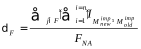
    </mixed-citation>
   </ref>
  </ref-list>
 </back>
</article>