<?xml version="1.0" encoding="UTF-8"?><!DOCTYPE article PUBLIC "-//NLM//DTD Journal Publishing DTD v3.0 20080202//EN" "http://dtd.nlm.nih.gov/publishing/3.0/journalpublishing3.dtd">
<article xmlns:mml="http://www.w3.org/1998/Math/MathML" xmlns:xlink="http://www.w3.org/1999/xlink" dtd-version="3.0" xml:lang="en" article-type="research article">
 <front>
  <journal-meta>
   <journal-id journal-id-type="publisher-id">
    wjet
   </journal-id>
   <journal-title-group>
    <journal-title>
     World Journal of Engineering and Technology
    </journal-title>
   </journal-title-group>
   <issn pub-type="epub">
    2331-4222
   </issn>
   <issn publication-format="print">
    2331-4249
   </issn>
   <publisher>
    <publisher-name>
     Scientific Research Publishing
    </publisher-name>
   </publisher>
  </journal-meta>
  <article-meta>
   <article-id pub-id-type="doi">
    10.4236/wjet.2024.124052
   </article-id>
   <article-id pub-id-type="publisher-id">
    wjet-136445
   </article-id>
   <article-categories>
    <subj-group subj-group-type="heading">
     <subject>
      Articles
     </subject>
    </subj-group>
    <subj-group subj-group-type="Discipline-v2">
     <subject>
      Chemistry 
     </subject>
     <subject>
       Materials Science, Engineering
     </subject>
    </subj-group>
   </article-categories>
   <title-group>
    Theoretical and Empirical Limits: Reexamining Betz’s Upper Limit towards a Practical Power Coefficients in Wind Turbines
    <sup>*</sup>
   </title-group>
   <contrib-group>
    <contrib contrib-type="author" xlink:type="simple">
     <name name-style="western">
      <surname>
       Richard M.
      </surname>
      <given-names>
       Kimiti
      </given-names>
     </name>
    </contrib>
    <contrib contrib-type="author" xlink:type="simple">
     <name name-style="western">
      <surname>
       Francis N.
      </surname>
      <given-names>
       Kariuki
      </given-names>
     </name>
    </contrib>
    <contrib contrib-type="author" xlink:type="simple">
     <name name-style="western">
      <surname>
       Joseph N.
      </surname>
      <given-names>
       Kamau
      </given-names>
     </name>
    </contrib>
    <contrib contrib-type="author" xlink:type="simple">
     <name name-style="western">
      <surname>
       Timonah N.
      </surname>
      <given-names>
       Soitah
      </given-names>
     </name>
    </contrib>
   </contrib-group> 
   <aff id="affnull">
    <addr-line>
     aDepartment of Physics, JKUAT University, Nairobi, Kenya
    </addr-line> 
   </aff> 
   <pub-date pub-type="epub">
    <day>
     04
    </day> 
    <month>
     09
    </month>
    <year>
     2024
    </year>
   </pub-date> 
   <volume>
    12
   </volume> 
   <issue>
    04
   </issue>
   <fpage>
    851
   </fpage>
   <lpage>
    866
   </lpage>
   <history>
    <date date-type="received">
     <day>
      17,
     </day>
     <month>
      August
     </month>
     <year>
      2024
     </year>
    </date>
    <date date-type="published">
     <day>
      27,
     </day>
     <month>
      August
     </month>
     <year>
      2024
     </year> 
    </date> 
    <date date-type="accepted">
     <day>
      27,
     </day>
     <month>
      September
     </month>
     <year>
      2024
     </year> 
    </date>
   </history>
   <permissions>
    <copyright-statement>
     © Copyright 2014 by authors and Scientific Research Publishing Inc. 
    </copyright-statement>
    <copyright-year>
     2014
    </copyright-year>
    <license>
     <license-p>
      This work is licensed under the Creative Commons Attribution International License (CC BY). http://creativecommons.org/licenses/by/4.0/
     </license-p>
    </license>
   </permissions>
   <abstract>
    The aspiration of all wind turbine designers is to attain Betz’s upper limit, which represents the highest efficiency in wind energy extraction. Majority of working turbines operate slightly below this limit with an exception of a few operating in wind tunnels. This study proposes for a comprehensive reevaluation of Betz’s derivation, aiming to establish the gap between a theoretical power limit and a practical limit for realization. There are two common expressions for power coefficient giving the same optimal value of 59%, but they generate different power-coefficient curves when plotted against velocity ratios. This paper presents a new method being referred as “Direct Multiplication Fractional Change” (DMFC) for deriving power-coefficient curves in wind energy, and compares its generated curve with established models. Discrepancies in power-coefficient expressions are identified and harmonized. Three approaches, namely EVAM, LVM, and DMFCM, were used for the numerical derivation of c
    <sub>p</sub> in the study, with their evaluation summarized in a table. The study collaborates its findings with a formulated velocity-distance curve, commonly presented as a hypothetical velocity profile in some publications. The results from DMFCM indicate two distinct maxima for the power coefficient. On the front side of the disc, a maximum of 0.5 is achievable in practice, although it is not the highest theoretically. On the rear side, a theoretical maximum of 0.59 is observed, but this value is not attainable in practice. These maxima are separated by their positions along the line of flow relative to the disc. However, this approximation is limited to a streamlined flow model of the rotor disc. 
   </abstract>
   <kwd-group> 
    <kwd>
     Wind Turbine
    </kwd> 
    <kwd>
      Betz’s Limit
    </kwd> 
    <kwd>
      Power Coefficient
    </kwd> 
    <kwd>
      Kinetic Pressure
    </kwd> 
    <kwd>
      Rotor Disc
    </kwd>
   </kwd-group>
  </article-meta>
 </front>
 <body>
  <sec id="s1">
   <title>1. Introduction</title>
   <p>Since 1926, Betz’s upper limit for wind power factor has never been disputed because most wind turbines operate between 75% - 85% of the Betz limit <xref ref-type="bibr" rid="scirp.136445-1">
     [1]
    </xref>. However, tidal turbines operating in a channel can theoretically attain a power coefficient several times larger than 16/27 <xref ref-type="bibr" rid="scirp.136445-2">
     [2]
    </xref> <xref ref-type="bibr" rid="scirp.136445-3">
     [3]
    </xref>, underscoring the potential for further refinement in design and operation. One suggested criterion for possibly attaining Betz’s upper limit is by using a thin disc with a solidity of 0.5 <xref ref-type="bibr" rid="scirp.136445-4">
     [4]
    </xref> in a CFD simulation. There are also some inconsistences detected when Betz’s model was reexamined and the main assumptions scrutinized <xref ref-type="bibr" rid="scirp.136445-5">
     [5]
    </xref>. One such inconsistence is the wind slowing down to zero velocity behind the rotor and the simple theory is no longer applicable. The major question is about how far the affected wind need to be slowed down to practically obtain this target <xref ref-type="bibr" rid="scirp.136445-6">
     [6]
    </xref>. The question further extends on whether this limit can be practically obtained or it is an ideal theoretical value <xref ref-type="bibr" rid="scirp.136445-7">
     [7]
    </xref>. There is a notable deviation between the theoretical design value and the actual value of the power coefficient because aerodynamic theory is still not completely correct <xref ref-type="bibr" rid="scirp.136445-6">
     [6]
    </xref>. Identifying the gap between theoretical ideals and practical application requires a thorough reexamination of Betz’s derivation and its assumptions. This study delves into the complexities of Betz’s limit and power coefficient expressions, identifying discrepancies and proposing a new derivation method to harmonize theoretical predictions with real-world performance. By scrutinizing existing methodologies and incorporating new insights, this research aims to enhance our understanding of wind turbine efficiency curves and pave the way for practical advancements in power coefficient optimization.</p>
   <p>
    <xref ref-type="bibr" rid="scirp.136445-"></xref>There are two main schools of thought in the derivation of Betz’s upper limit and both are in agreement about the value of 0.59, but they diverge on the extent into which to slow down the upstream wind in order to achieve this limit.</p>
   <p>The first school of thought is based on a linear momentum theory. There is a conservation of work done in expanding the stream of flow downstream and therefore, Bernoulli’s equation for upstream section is equated to that of downstream section to obtain pressure difference as shown in (1.1).</p>
   <p>
    <math display="inline" xmlns="http://www.w3.org/1998/Math/MathML"> <mrow> 
      <mi>
        Δ 
      </mi> 
      <mi>
        p 
      </mi> 
      <mo>
        = 
      </mo> 
      <mfrac> 
       <mn>
         1 
       </mn> 
       <mn>
         2 
       </mn> 
      </mfrac> 
      <mi>
        ρ 
      </mi> 
      <mrow> 
       <mo>
         ( 
       </mo> 
       <mrow> 
        <msubsup> 
         <mi>
           u 
         </mi> 
         <mn>
           1 
         </mn> 
         <mn>
           2 
         </mn> 
        </msubsup> 
        <mo>
          − 
        </mo> 
        <msubsup> 
         <mi>
           u 
         </mi> 
         <mn>
           4 
         </mn> 
         <mn>
           2 
         </mn> 
        </msubsup> 
       </mrow> 
       <mo>
         ) 
       </mo> 
      </mrow> 
     </mrow> 
    </math> (1.1)</p>
   <p>where, ∆p is pressure difference, 
    <math display="inline" xmlns="http://www.w3.org/1998/Math/MathML"> <mi>
       ρ 
     </mi> 
    </math> is the density of air, 
    <math display="inline" xmlns="http://www.w3.org/1998/Math/MathML"> <mrow> 
      <msub> 
       <mi>
         u 
       </mi> 
       <mn>
         1 
       </mn> 
      </msub> 
     </mrow> 
    </math> is the undisturbed wind velocity upstream and 
    <math display="inline" xmlns="http://www.w3.org/1998/Math/MathML"> <mrow> 
      <msub> 
       <mi>
         u 
       </mi> 
       <mn>
         2 
       </mn> 
      </msub> 
     </mrow> 
    </math> is the lowest wind velocity downstream.</p>
   <p>Power extracted is a product of pressure difference, the cross-sectional area and velocity as given in Equation (1.2).</p>
   <p>
    <math display="inline" xmlns="http://www.w3.org/1998/Math/MathML"> <mrow> 
      <mi>
        P 
      </mi> 
      <mo>
        = 
      </mo> 
      <mfrac> 
       <mn>
         1 
       </mn> 
       <mn>
         2 
       </mn> 
      </mfrac> 
      <mi>
        ρ 
      </mi> 
      <msub> 
       <mi>
         A 
       </mi> 
       <mn>
         1 
       </mn> 
      </msub> 
      <mrow> 
       <mo>
         ( 
       </mo> 
       <mrow> 
        <msubsup> 
         <mi>
           u 
         </mi> 
         <mn>
           1 
         </mn> 
         <mn>
           2 
         </mn> 
        </msubsup> 
        <mo>
          − 
        </mo> 
        <msubsup> 
         <mi>
           u 
         </mi> 
         <mn>
           4 
         </mn> 
         <mn>
           2 
         </mn> 
        </msubsup> 
       </mrow> 
       <mo>
         ) 
       </mo> 
      </mrow> 
      <msub> 
       <mi>
         u 
       </mi> 
       <mn>
         2 
       </mn> 
      </msub> 
     </mrow> 
    </math> (1.2)</p>
   <p>where, P is the extracted power, 
    <math display="inline" xmlns="http://www.w3.org/1998/Math/MathML"> <mrow> 
      <msub> 
       <mi>
         A 
       </mi> 
       <mn>
         1 
       </mn> 
      </msub> 
     </mrow> 
    </math> is the upstream cross-sectional area and 
    <math display="inline" xmlns="http://www.w3.org/1998/Math/MathML"> <mrow> 
      <msub> 
       <mi>
         u 
       </mi> 
       <mn>
         2 
       </mn> 
      </msub> 
     </mrow> 
    </math> is the instantaneous velocity at the turbine.</p>
   <p>A fractional change in velocity also referred as axial induction factor, a is introduced in the analysis. Axial induction factor a is defined by Equation (1.3).</p>
   <p>
    <math display="inline" xmlns="http://www.w3.org/1998/Math/MathML"> <mrow> 
      <mi>
        a 
      </mi> 
      <mo>
        = 
      </mo> 
      <mfrac> 
       <mrow> 
        <msub> 
         <mi>
           u 
         </mi> 
         <mn>
           1 
         </mn> 
        </msub> 
        <mo>
          − 
        </mo> 
        <mi>
          u 
        </mi> 
       </mrow> 
       <mrow> 
        <msub> 
         <mi>
           u 
         </mi> 
         <mn>
           1 
         </mn> 
        </msub> 
       </mrow> 
      </mfrac> 
     </mrow> 
    </math> (1.3)</p>
   <p>where; u<sub>1</sub> is the undisturbed wind velocity upstream and u is the instantaneous velocity after disturbance.</p>
   <p>The power coefficient 
    <math display="inline" xmlns="http://www.w3.org/1998/Math/MathML"> <mrow> 
      <msub> 
       <mi>
         C 
       </mi> 
       <mi>
         P 
       </mi> 
      </msub> 
     </mrow> 
    </math> using this approach is given by Equation (1.4).</p>
   <p>
    <math display="inline" xmlns="http://www.w3.org/1998/Math/MathML"> <mrow> 
      <msub> 
       <mi>
         C 
       </mi> 
       <mi>
         P 
       </mi> 
      </msub> 
      <mo>
        = 
      </mo> 
      <mn>
        4 
      </mn> 
      <mi>
        a 
      </mi> 
      <msup> 
       <mrow> 
        <mrow> 
         <mo>
           ( 
         </mo> 
         <mrow> 
          <mn>
            1 
          </mn> 
          <mo>
            − 
          </mo> 
          <mi>
            a 
          </mi> 
         </mrow> 
         <mo>
           ) 
         </mo> 
        </mrow> 
       </mrow> 
       <mn>
         2 
       </mn> 
      </msup> 
     </mrow> 
    </math> (1.4)</p>
   <p>The actuator factor a has an optimum value of one third hence placing the Betz’s limit to be attained when the upstream wind is slowed down to two thirds of the undisturbed velocity <xref ref-type="bibr" rid="scirp.136445-7">
     [7]
    </xref>-<xref ref-type="bibr" rid="scirp.136445-9">
     [9]
    </xref>. Betz’s upper limit occurs at an axial induction factor of 
    <math display="inline" xmlns="http://www.w3.org/1998/Math/MathML"> <mrow> 
      <mn>
        0.3 
      </mn> 
      <mover accent="true"> 
       <mn>
         3 
       </mn> 
       <mo>
         ˙ 
       </mo> 
      </mover> 
     </mrow> 
    </math> as shown in <xref ref-type="fig" rid="fig1(a)">
     Figure 1(a)
    </xref>, but at velocity fraction of 
    <math display="inline" xmlns="http://www.w3.org/1998/Math/MathML"> <mrow> 
      <mn>
        0.6 
      </mn> 
      <mover accent="true"> 
       <mn>
         6 
       </mn> 
       <mo>
         ˙ 
       </mo> 
      </mover> 
     </mrow> 
    </math> as shown in <xref ref-type="fig" rid="fig1(b)">
     Figure 1(b)
    </xref>.</p>
   <fig id="fig1" position="float">
    <label>Figure 1</label>
    <caption>
     <title>Figure 1. (a) Power coefficient against induction factor (b) Power coefficient against velocity fraction <xref ref-type="bibr" rid="scirp.136445-8">
       [8]
      </xref>-<xref ref-type="bibr" rid="scirp.136445-10">
       [10]
      </xref>.</title>
    </caption>
    <graphic mimetype="image" position="float" xlink:type="simple" xlink:href="https://html.scirp.org/file/1561574-rId38.jpeg?20240930021344" />
   </fig>
   <p>The curve in <xref ref-type="fig" rid="fig1(b)">
     Figure 1(b)
    </xref> predicts zero power will be extracted when affected wind velocity is slowed down to zero. This is in contrast with the realistic expectation that power coefficient should reach 100% if all the kinetic energy of the wind is fully harnessed.</p>
   <p>In this study, we designate this method as the Extreme Values Approximation Method (EVAM) for identification purposes. The analysis considers the maximum change in static pressure downstream and the minimum cross-sectional area of the flow upstream.</p>
   <p>The second school of thought is also based on conservation of linear momentum but velocity at the disc is the average of the upstream and downstream wind speeds as shown in Equation (1.5).</p>
   <p>
    <math display="inline" xmlns="http://www.w3.org/1998/Math/MathML"> <mrow> 
      <msub> 
       <mi>
         u 
       </mi> 
       <mn>
         2 
       </mn> 
      </msub> 
      <mo>
        = 
      </mo> 
      <mfrac> 
       <mn>
         1 
       </mn> 
       <mn>
         2 
       </mn> 
      </mfrac> 
      <mrow> 
       <mo>
         ( 
       </mo> 
       <mrow> 
        <msub> 
         <mi>
           u 
         </mi> 
         <mn>
           1 
         </mn> 
        </msub> 
        <mo>
          + 
        </mo> 
        <msub> 
         <mi>
           u 
         </mi> 
         <mn>
           4 
         </mn> 
        </msub> 
       </mrow> 
       <mo>
         ) 
       </mo> 
      </mrow> 
     </mrow> 
    </math> (1.5)</p>
   <p>Another difference is the consideration of the cross-sectional area at the turbine 
    <math display="inline" xmlns="http://www.w3.org/1998/Math/MathML"> <mrow> 
      <msub> 
       <mi>
         A 
       </mi> 
       <mn>
         2 
       </mn> 
      </msub> 
     </mrow> 
    </math> which is 1.5 of the upstream area 
    <math display="inline" xmlns="http://www.w3.org/1998/Math/MathML"> <mrow> 
      <msub> 
       <mi>
         A 
       </mi> 
       <mn>
         1 
       </mn> 
      </msub> 
     </mrow> 
    </math>. The variables used to obtain power (pressure, area and velocity) in this method are all localized at the disk position and, therefore, identified as Localized Values Method (LVM).</p>
   <p>Extracted power in LVM method is given by Equation (1.6).</p>
   <p>
    <math display="inline" xmlns="http://www.w3.org/1998/Math/MathML"> <mrow> 
      <mi>
        P 
      </mi> 
      <mo>
        = 
      </mo> 
      <mfrac> 
       <mn>
         1 
       </mn> 
       <mn>
         2 
       </mn> 
      </mfrac> 
      <mi>
        ρ 
      </mi> 
      <msub> 
       <mi>
         A 
       </mi> 
       <mn>
         2 
       </mn> 
      </msub> 
      <mrow> 
       <mo>
         ( 
       </mo> 
       <mrow> 
        <msubsup> 
         <mi>
           u 
         </mi> 
         <mn>
           1 
         </mn> 
         <mn>
           2 
         </mn> 
        </msubsup> 
        <mo>
          − 
        </mo> 
        <msubsup> 
         <mi>
           u 
         </mi> 
         <mn>
           2 
         </mn> 
         <mn>
           2 
         </mn> 
        </msubsup> 
       </mrow> 
       <mo>
         ) 
       </mo> 
      </mrow> 
      <mrow> 
       <mo>
         ( 
       </mo> 
       <mrow> 
        <msub> 
         <mi>
           u 
         </mi> 
         <mn>
           1 
         </mn> 
        </msub> 
        <mo>
          − 
        </mo> 
        <msub> 
         <mi>
           u 
         </mi> 
         <mn>
           2 
         </mn> 
        </msub> 
       </mrow> 
       <mo>
         ) 
       </mo> 
      </mrow> 
     </mrow> 
    </math> (1.6)</p>
   <p>where, P is the extracted power, 
    <math display="inline" xmlns="http://www.w3.org/1998/Math/MathML"> <mrow> 
      <msub> 
       <mi>
         A 
       </mi> 
       <mn>
         2 
       </mn> 
      </msub> 
     </mrow> 
    </math> is the cross-sectional area at the turbine, 
    <math display="inline" xmlns="http://www.w3.org/1998/Math/MathML"> <mrow> 
      <msub> 
       <mi>
         u 
       </mi> 
       <mn>
         2 
       </mn> 
      </msub> 
     </mrow> 
    </math> is the instantaneous velocity at the turbine and 
    <math display="inline" xmlns="http://www.w3.org/1998/Math/MathML"> <mrow> 
      <msub> 
       <mi>
         u 
       </mi> 
       <mn>
         1 
       </mn> 
      </msub> 
     </mrow> 
    </math> is the undisturbed wind upstream.</p>
   <p>The concept of velocity fraction, b is introduced to solve for power coefficient. Equation (1.7) shows velocity fraction representing the reduction in wind speed due to the extraction of wind energy.</p>
   <p>
    <math display="inline" xmlns="http://www.w3.org/1998/Math/MathML"> <mrow> 
      <mi>
        b 
      </mi> 
      <mo>
        = 
      </mo> 
      <mfrac> 
       <mi>
         v 
       </mi> 
       <mrow> 
        <msub> 
         <mi>
           v 
         </mi> 
         <mn>
           1 
         </mn> 
        </msub> 
       </mrow> 
      </mfrac> 
     </mrow> 
    </math> (1.7)</p>
   <p>where; 
    <math display="inline" xmlns="http://www.w3.org/1998/Math/MathML"> <mrow> 
      <msub> 
       <mi>
         v 
       </mi> 
       <mn>
         1 
       </mn> 
      </msub> 
     </mrow> 
    </math> is the undisturbed wind velocity upstream and v is the instantaneous velocity after disturbance.</p>
   <p>Power coefficient in this LVM approach is given by Equation (1.8).</p>
   <p>
    <math display="inline" xmlns="http://www.w3.org/1998/Math/MathML"> <mrow> 
      <msub> 
       <mi>
         C 
       </mi> 
       <mi>
         p 
       </mi> 
      </msub> 
      <mo>
        = 
      </mo> 
      <mfrac> 
       <mn>
         1 
       </mn> 
       <mn>
         2 
       </mn> 
      </mfrac> 
      <mrow> 
       <mo>
         ( 
       </mo> 
       <mrow> 
        <mn>
          1 
        </mn> 
        <mo>
          + 
        </mo> 
        <mi>
          b 
        </mi> 
       </mrow> 
       <mo>
         ) 
       </mo> 
      </mrow> 
      <mrow> 
       <mo>
         ( 
       </mo> 
       <mrow> 
        <mn>
          1 
        </mn> 
        <mo>
          − 
        </mo> 
        <msup> 
         <mi>
           b 
         </mi> 
         <mn>
           2 
         </mn> 
        </msup> 
       </mrow> 
       <mo>
         ) 
       </mo> 
      </mrow> 
     </mrow> 
    </math> (1.8)</p>
   <p>In this LVM approach, the Betz’s upper limit occurs at velocity fraction of 
    <math display="inline" xmlns="http://www.w3.org/1998/Math/MathML"> <mrow> 
      <mn>
        0.3 
      </mn> 
      <mover accent="true"> 
       <mn>
         3 
       </mn> 
       <mo>
         ˙ 
       </mo> 
      </mover> 
     </mrow> 
    </math> as shown in <xref ref-type="fig" rid="fig2">
     Figure 2
    </xref>. The curve also predicts a power coefficient of 0.5 when wind particles are totally slowed to zero velocity.</p>
   <fig id="fig2" position="float">
    <label>Figure 2</label>
    <caption>
     <title>Figure 2. Power coefficient against velocity fraction <xref ref-type="bibr" rid="scirp.136445-11">
       [11]
      </xref> <xref ref-type="bibr" rid="scirp.136445-12">
       [12]
      </xref>.</title>
    </caption>
    <graphic mimetype="image" position="float" xlink:type="simple" xlink:href="https://html.scirp.org/file/1561574-rId60.jpeg?20240930021344" />
   </fig>
   <p>A correct interpretation of this curve indicates that a higher power of 0.59 can be extracted at a third of the undisturbed wind compared to 0.5 when wind loses its total kinetic energy. This is practically a contradiction. The highest actual power coefficient ranges between 0.45 and 0.50 <xref ref-type="bibr" rid="scirp.136445-1">
     [1]
    </xref>. To add on the controversy, it is practically not possible to slow down wind below a factor of 0.5 by use of an obstacle hence questioning the possibility of one thirds of the undisturbed velocity <xref ref-type="bibr" rid="scirp.136445-8">
     [8]
    </xref> <xref ref-type="bibr" rid="scirp.136445-13">
     [13]
    </xref>.</p>
   <p>
    <xref ref-type="bibr" rid="scirp.136445-"></xref>Both EVAM and LVM disagree with hypothetical velocity-distance curve which is used to explain velocity profile along the line of flow. <xref ref-type="fig" rid="fig3(a)">
     Figure 3(a)
    </xref> shows the actuator disc model with discrete velocities ( 
    <math display="inline" xmlns="http://www.w3.org/1998/Math/MathML"> <mrow> 
      <msub> 
       <mi>
         u 
       </mi> 
       <mn>
         1 
       </mn> 
      </msub> 
     </mrow> 
    </math>, 
    <math display="inline" xmlns="http://www.w3.org/1998/Math/MathML"> <mrow> 
      <msub> 
       <mi>
         u 
       </mi> 
       <mn>
         2 
       </mn> 
      </msub> 
     </mrow> 
    </math>, 
    <math display="inline" xmlns="http://www.w3.org/1998/Math/MathML"> <mrow> 
      <msub> 
       <mi>
         u 
       </mi> 
       <mn>
         3 
       </mn> 
      </msub> 
     </mrow> 
    </math> and 
    <math display="inline" xmlns="http://www.w3.org/1998/Math/MathML"> <mrow> 
      <msub> 
       <mi>
         u 
       </mi> 
       <mn>
         4 
       </mn> 
      </msub> 
     </mrow> 
    </math>) and corresponding kinetic pressures ( 
    <math display="inline" xmlns="http://www.w3.org/1998/Math/MathML"> <mrow> 
      <msub> 
       <mi>
         p 
       </mi> 
       <mn>
         1 
       </mn> 
      </msub> 
     </mrow> 
    </math>, 
    <math display="inline" xmlns="http://www.w3.org/1998/Math/MathML"> <mrow> 
      <msub> 
       <mi>
         p 
       </mi> 
       <mn>
         2 
       </mn> 
      </msub> 
     </mrow> 
    </math>, 
    <math display="inline" xmlns="http://www.w3.org/1998/Math/MathML"> <mrow> 
      <msub> 
       <mi>
         p 
       </mi> 
       <mn>
         3 
       </mn> 
      </msub> 
     </mrow> 
    </math> and 
    <math display="inline" xmlns="http://www.w3.org/1998/Math/MathML"> <mrow> 
      <msub> 
       <mi>
         p 
       </mi> 
       <mn>
         4 
       </mn> 
      </msub> 
     </mrow> 
    </math>) of the wind from upstream to downstream. The minimum velocity downstream is one third of the undisturbed wind and this occurs behind the rotor disc as shown in <xref ref-type="fig" rid="fig3(b)">
     Figure 3(b)
    </xref>.</p>
   <fig id="fig3" position="float">
    <label>Figure 3</label>
    <caption>
     <title>Figure 3. (a) Actuator disc model of a wind turbine, (b) Hypothetical velocity graph <xref ref-type="bibr" rid="scirp.136445-8">
       [8]
      </xref>.</title>
    </caption>
    <graphic mimetype="image" position="float" xlink:type="simple" xlink:href="https://html.scirp.org/file/1561574-rId76.jpeg?20240930021344" />
   </fig>
   <p>
    <xref ref-type="bibr" rid="scirp.136445-"></xref>From the hypothetical velocity graph and considering the distance to be positive upstream and negative downstream, the Betz’s limit practically occurs behind the disc at an instantaneous velocity of negative a third of the upstream wind. This is in contrast with EVAM method where the axial induction factor, a has its optimum at positive one third and not at negative one third. Hypothetical velocity-distance profile is in agreement with the LVM methods where wind velocity is slowed down to a factor of 
    <math display="inline" xmlns="http://www.w3.org/1998/Math/MathML"> <mrow> 
      <mn>
        0.6 
      </mn> 
      <mover accent="true"> 
       <mn>
         6 
       </mn> 
       <mo>
         ˙ 
       </mo> 
      </mover> 
     </mrow> 
    </math> at the rotor disc. However, there is a further decrease in velocity as wind occupy the low-pressure region (almost a vacuum) behind the disc. The wind particles past the disc lose their energy to the air mass within the low-pressure region. The algebraic resulting velocity should be a third of the undisturbed velocity after combining the velocities behind the disc according to this hypothetical velocity-distance curve. Wind will eventually recover its velocity downstream as shown in <xref ref-type="fig" rid="fig3(b)">
     Figure 3(b)
    </xref>. In this paper, a velocity-distance function is formulated to confirm this hypothetical velocity curve. The formulated function was used to perform simulations and accurately determine affected distances both upstream to downstream. The velocity of the wind, angle of attack and the radius of the turbine were the factors considered in the simulation.</p>
  </sec><sec id="s2">
   <title>2. Numerical Proposal</title>
   <sec id="s2_1">
    <title>2.1. Derivation of Power Coefficient</title>
    <p>The paper introduces a new approach being referred as Direct Multiplication Fractional Changes Method (DMFCM) in the derivation of power coefficient. Wind energy extraction process involves conversion of the kinetic energy of the wind into mechanical energy of the rotor. An actuator disc model is commonly used in the derivation of power coefficient and it is a representation of an ideal horizontal-axis wind turbine. Power from the wind is a product of force and velocity. Force from wind is the change in kinetic pressure multiplied by the effective cross-section area. Therefore, the three variables used in calculation of wind power are given by Equation (2.1).</p>
    <p>
     <math display="inline" xmlns="http://www.w3.org/1998/Math/MathML"> <mrow> 
       <mi>
         P 
       </mi> 
       <mo>
         = 
       </mo> 
       <mi>
         p 
       </mi> 
       <mi>
         A 
       </mi> 
       <mi>
         v 
       </mi> 
      </mrow> 
     </math> (2.1)</p>
    <p>where; P is the power, p is the kinetic pressure and v is the wind velocity.</p>
    <p>The new approach considers fractional change of each variable that constitute wind power. These individual fractional changes are directly multiplied to obtain the overall fractional change in power. An assumption in this approach is that a flow sensor attached to the turbine blades can accurately measure instantaneous velocity.</p>
    <p>A fractional change in power can, therefore, be expressed as direct multiplication of individual fractional changes (DMFCM) for the variables as shown in Equation (2.2).</p>
    <p>
     <math display="inline" xmlns="http://www.w3.org/1998/Math/MathML"> <mrow> 
       <mfrac> 
        <mrow> 
         <mi>
           Δ 
         </mi> 
         <mi>
           P 
         </mi> 
        </mrow> 
        <mi>
          P 
        </mi> 
       </mfrac> 
       <mo>
         = 
       </mo> 
       <mfrac> 
        <mrow> 
         <mi>
           Δ 
         </mi> 
         <mi>
           p 
         </mi> 
        </mrow> 
        <mi>
          p 
        </mi> 
       </mfrac> 
       <mo>
         ⋅ 
       </mo> 
       <mfrac> 
        <mrow> 
         <mi>
           Δ 
         </mi> 
         <mi>
           A 
         </mi> 
        </mrow> 
        <mi>
          A 
        </mi> 
       </mfrac> 
       <mo>
         ⋅ 
       </mo> 
       <mfrac> 
        <mrow> 
         <mi>
           Δ 
         </mi> 
         <mi>
           v 
         </mi> 
        </mrow> 
        <mi>
          v 
        </mi> 
       </mfrac> 
      </mrow> 
     </math> (2.2)</p>
    <p>where: ∆P is change in power, ∆p is change in pressure, ∆A is the change in cross-sectional area, and ∆v is the change in velocity.</p>
    <p>Kinetic pressure, p at a given velocity is given by Equation (2.3).</p>
    <p>
     <math display="inline" xmlns="http://www.w3.org/1998/Math/MathML"> <mrow> 
       <mi>
         p 
       </mi> 
       <mo>
         = 
       </mo> 
       <mfrac> 
        <mn>
          1 
        </mn> 
        <mn>
          2 
        </mn> 
       </mfrac> 
       <mi>
         ρ 
       </mi> 
       <msup> 
        <mi>
          v 
        </mi> 
        <mn>
          2 
        </mn> 
       </msup> 
      </mrow> 
     </math> (2.3)</p>
    <p>where; 
     <math display="inline" xmlns="http://www.w3.org/1998/Math/MathML"> <mi>
        ρ 
      </mi> 
     </math> is the density of air and v is the instantaneous velocity.</p>
    <p>Kinetic pressure decreases downstream and it is converted into static pressure. Therefore, kinetic pressure at the rotor disc, 
     <math display="inline" xmlns="http://www.w3.org/1998/Math/MathML"> <mrow> 
       <msub> 
        <mi>
          p 
        </mi> 
        <mn>
          2 
        </mn> 
       </msub> 
      </mrow> 
     </math> is less than upstream kinetic pressure 
     <math display="inline" xmlns="http://www.w3.org/1998/Math/MathML"> <mrow> 
       <msub> 
        <mi>
          p 
        </mi> 
        <mn>
          1 
        </mn> 
       </msub> 
      </mrow> 
     </math> as shown in <xref ref-type="fig" rid="fig3">
      Figure 3
     </xref>. The fractional change in kinetic pressure at the turbine is given by Equation (2.4).</p>
    <p>
     <math display="inline" xmlns="http://www.w3.org/1998/Math/MathML"> <mrow> 
       <mfrac> 
        <mrow> 
         <mi>
           Δ 
         </mi> 
         <mi>
           p 
         </mi> 
        </mrow> 
        <mi>
          p 
        </mi> 
       </mfrac> 
       <mo>
         = 
       </mo> 
       <mfrac> 
        <mrow> 
         <msubsup> 
          <mi>
            v 
          </mi> 
          <mn>
            2 
          </mn> 
          <mn>
            2 
          </mn> 
         </msubsup> 
         <mo>
           − 
         </mo> 
         <msubsup> 
          <mi>
            v 
          </mi> 
          <mn>
            1 
          </mn> 
          <mn>
            2 
          </mn> 
         </msubsup> 
        </mrow> 
        <mrow> 
         <msubsup> 
          <mi>
            v 
          </mi> 
          <mn>
            1 
          </mn> 
          <mn>
            2 
          </mn> 
         </msubsup> 
        </mrow> 
       </mfrac> 
      </mrow> 
     </math> (2.4)</p>
    <p>where: 
     <math display="inline" xmlns="http://www.w3.org/1998/Math/MathML"> <mrow> 
       <msub> 
        <mi>
          v 
        </mi> 
        <mn>
          2 
        </mn> 
       </msub> 
      </mrow> 
     </math> is the velocity at the turbine and 
     <math display="inline" xmlns="http://www.w3.org/1998/Math/MathML"> <mrow> 
       <msub> 
        <mi>
          v 
        </mi> 
        <mn>
          1 
        </mn> 
       </msub> 
      </mrow> 
     </math> is the velocity upstream.</p>
    <p>Slowing down wind causes the flow stream to expand downstream because of conversion of kinetic pressure into static pressure. The affected cross-section area 
     <math display="inline" xmlns="http://www.w3.org/1998/Math/MathML"> <mrow> 
       <msub> 
        <mi>
          A 
        </mi> 
        <mn>
          1 
        </mn> 
       </msub> 
      </mrow> 
     </math> upstream is two thirds of the rotor disc 
     <math display="inline" xmlns="http://www.w3.org/1998/Math/MathML"> <mrow> 
       <msub> 
        <mi>
          A 
        </mi> 
        <mn>
          2 
        </mn> 
       </msub> 
      </mrow> 
     </math> <xref ref-type="bibr" rid="scirp.136445-8">
      [8]
     </xref>. The fractional change in cross-sectional area is given as Equation (2.5).</p>
    <p>
     <math display="inline" xmlns="http://www.w3.org/1998/Math/MathML"> <mrow> 
       <mfrac> 
        <mrow> 
         <mi>
           Δ 
         </mi> 
         <mi>
           A 
         </mi> 
        </mrow> 
        <mi>
          A 
        </mi> 
       </mfrac> 
       <mo>
         = 
       </mo> 
       <mfrac> 
        <mrow> 
         <msub> 
          <mi>
            A 
          </mi> 
          <mn>
            2 
          </mn> 
         </msub> 
         <mo>
           − 
         </mo> 
         <msub> 
          <mi>
            A 
          </mi> 
          <mn>
            1 
          </mn> 
         </msub> 
        </mrow> 
        <mrow> 
         <msub> 
          <mi>
            A 
          </mi> 
          <mn>
            1 
          </mn> 
         </msub> 
        </mrow> 
       </mfrac> 
       <mo>
         = 
       </mo> 
       <mfrac> 
        <mn>
          1 
        </mn> 
        <mn>
          2 
        </mn> 
       </mfrac> 
       <mo> 
       </mo> 
      </mrow> 
     </math> (2.5)</p>
    <p>The fractional change in velocity is given as Equation (2.6).</p>
    <p>
     <math display="inline" xmlns="http://www.w3.org/1998/Math/MathML"> <mrow> 
       <mfrac> 
        <mrow> 
         <mi>
           Δ 
         </mi> 
         <mi>
           v 
         </mi> 
        </mrow> 
        <mi>
          v 
        </mi> 
       </mfrac> 
       <mo>
         = 
       </mo> 
       <mfrac> 
        <mrow> 
         <msub> 
          <mi>
            v 
          </mi> 
          <mn>
            2 
          </mn> 
         </msub> 
         <mo>
           − 
         </mo> 
         <msub> 
          <mi>
            v 
          </mi> 
          <mn>
            1 
          </mn> 
         </msub> 
        </mrow> 
        <mrow> 
         <msub> 
          <mi>
            v 
          </mi> 
          <mn>
            1 
          </mn> 
         </msub> 
        </mrow> 
       </mfrac> 
      </mrow> 
     </math> (2.6)</p>
    <p>Substituting Equations (2.4) - (2.6) into Equation (2.2) gives Equation (2.7).</p>
    <p>
     <math display="inline" xmlns="http://www.w3.org/1998/Math/MathML"> <mrow> 
       <mfrac> 
        <mrow> 
         <mi>
           Δ 
         </mi> 
         <mi>
           P 
         </mi> 
        </mrow> 
        <mi>
          P 
        </mi> 
       </mfrac> 
       <mo>
         = 
       </mo> 
       <mfrac> 
        <mn>
          1 
        </mn> 
        <mn>
          2 
        </mn> 
       </mfrac> 
       <mo>
         ⋅ 
       </mo> 
       <mfrac> 
        <mrow> 
         <msubsup> 
          <mi>
            v 
          </mi> 
          <mn>
            2 
          </mn> 
          <mn>
            2 
          </mn> 
         </msubsup> 
         <mo>
           − 
         </mo> 
         <msubsup> 
          <mi>
            v 
          </mi> 
          <mn>
            1 
          </mn> 
          <mn>
            2 
          </mn> 
         </msubsup> 
        </mrow> 
        <mrow> 
         <msubsup> 
          <mi>
            v 
          </mi> 
          <mn>
            1 
          </mn> 
          <mn>
            2 
          </mn> 
         </msubsup> 
        </mrow> 
       </mfrac> 
       <mo>
         ⋅ 
       </mo> 
       <mfrac> 
        <mrow> 
         <msub> 
          <mi>
            v 
          </mi> 
          <mn>
            2 
          </mn> 
         </msub> 
         <mo>
           − 
         </mo> 
         <msub> 
          <mi>
            v 
          </mi> 
          <mn>
            1 
          </mn> 
         </msub> 
        </mrow> 
        <mrow> 
         <msub> 
          <mi>
            v 
          </mi> 
          <mn>
            1 
          </mn> 
         </msub> 
        </mrow> 
       </mfrac> 
       <mo>
         = 
       </mo> 
       <mfrac> 
        <mn>
          1 
        </mn> 
        <mn>
          2 
        </mn> 
       </mfrac> 
       <mrow> 
        <mo>
          ( 
        </mo> 
        <mrow> 
         <msup> 
          <mi>
            b 
          </mi> 
          <mn>
            2 
          </mn> 
         </msup> 
         <mo>
           − 
         </mo> 
         <mn>
           1 
         </mn> 
        </mrow> 
        <mo>
          ) 
        </mo> 
       </mrow> 
       <mrow> 
        <mo>
          ( 
        </mo> 
        <mrow> 
         <mi>
           b 
         </mi> 
         <mo>
           − 
         </mo> 
         <mn>
           1 
         </mn> 
        </mrow> 
        <mo>
          ) 
        </mo> 
       </mrow> 
      </mrow> 
     </math> (2.7)</p>
    <p>where: b is a ratio of velocity at the disc, 
     <math display="inline" xmlns="http://www.w3.org/1998/Math/MathML"> <mrow> 
       <msub> 
        <mi>
          v 
        </mi> 
        <mn>
          2 
        </mn> 
       </msub> 
      </mrow> 
     </math> divided by undisturbed velocity, 
     <math display="inline" xmlns="http://www.w3.org/1998/Math/MathML"> <mrow> 
       <msub> 
        <mi>
          v 
        </mi> 
        <mn>
          1 
        </mn> 
       </msub> 
      </mrow> 
     </math>.</p>
    <p>
     <xref ref-type="fig" rid="fig4">
      Figure 4
     </xref> shows power coefficient curve from Equation (2.7). It is a new curve illustrating how power coefficient changes from undisturbed wind upstream, +b up to a fully recovered wind downstream, −b behind the disc.</p>
    <fig id="fig4" position="float">
     <label>Figure 4</label>
     <caption>
      <title>Figure 4. Power coefficient against velocity fraction using DMFC method.</title>
     </caption>
     <graphic mimetype="image" position="float" xlink:type="simple" xlink:href="https://html.scirp.org/file/1561574-rId108.jpeg?20240930021344" />
    </fig>
    <p>
     <xref ref-type="bibr" rid="scirp.136445-"></xref>The optimum power coefficient in <xref ref-type="fig" rid="fig4">
      Figure 4
     </xref> is in agreement with the hypothetical velocity curve where the minimum velocity occurs downstream and is one third of the undisturbed wind as shown in <xref ref-type="fig" rid="fig3(b)">
      Figure 3(b)
     </xref>. Considering the distance to be positive upstream and negative downstream, the Betz’s limit can practically occur behind the disc at an instant velocity of negative a third of the undisturbed wind. It is impossible to extract power behind the disc and therefore the Betz’s limit is an ideal theoretical value. If the hypothetical velocity curve is correctly formulated, it will be possible to predict the distance behind the disc where slowing wind will have its minimum velocity.</p>
   </sec>
   <sec id="s2_2">
    <title>
     <xref ref-type="bibr" rid="scirp.136445-"></xref>2.2. Formulating the Hypothetical Velocity Curve</title>
    <p>
     <xref ref-type="bibr" rid="scirp.136445-"></xref>Velocity is a vector quantity with both directions and magnitude. Wind velocity reduces downstream changing both in magnitude and direction. Assuming the flow is streamlined and there is no rotating wake, wind velocity is modelled as a vector quantity that is undergoing geometrical transformation at different positions in the direction of flow downstream as shown in <xref ref-type="fig" rid="fig5">
      Figure 5
     </xref>.</p>
    <fig id="fig5" position="float">
     <label>Figure 5</label>
     <caption>
      <title>Figure 5. Wind velocity as a vector geometrical transformation downstream.</title>
     </caption>
     <graphic mimetype="image" position="float" xlink:type="simple" xlink:href="https://html.scirp.org/file/1561574-rId109.jpeg?20240930021345" />
    </fig>
    <p>Some of undisturbed wind 
     <math display="inline" xmlns="http://www.w3.org/1998/Math/MathML"> <mrow> 
       <msub> 
        <mi>
          v 
        </mi> 
        <mn>
          1 
        </mn> 
       </msub> 
      </mrow> 
     </math> temporarily stops to form an air wedge when it is blocked by the rotor disc. The wind direction will be diverted through an angle 
     <math display="inline" xmlns="http://www.w3.org/1998/Math/MathML"> <mi>
        θ 
      </mi> 
     </math> and the magnitude reduced to 
     <math display="inline" xmlns="http://www.w3.org/1998/Math/MathML"> <mrow> 
       <msub> 
        <mi>
          v 
        </mi> 
        <mn>
          2 
        </mn> 
       </msub> 
       <mo>
         = 
       </mo> 
       <msub> 
        <mi>
          v 
        </mi> 
        <mn>
          1 
        </mn> 
       </msub> 
       <mi>
         cos 
       </mi> 
       <mi>
         θ 
       </mi> 
      </mrow> 
     </math>. Past the edges of the rotor disc, the wind vector returns to its original direction (horizontal) further reducing the magnitude to 
     <math display="inline" xmlns="http://www.w3.org/1998/Math/MathML"> <mrow> 
       <msub> 
        <mi>
          v 
        </mi> 
        <mn>
          3 
        </mn> 
       </msub> 
       <mo>
         = 
       </mo> 
       <msub> 
        <mi>
          v 
        </mi> 
        <mn>
          1 
        </mn> 
       </msub> 
       <msup> 
        <mrow> 
         <mi>
           cos 
         </mi> 
        </mrow> 
        <mn>
          2 
        </mn> 
       </msup> 
       <mi>
         θ 
       </mi> 
      </mrow> 
     </math>. There is a low-pressure region behind the disc and some wind particles in this region are not in motion. The wind velocity vector past the edges will be diverted again to vector 
     <math display="inline" xmlns="http://www.w3.org/1998/Math/MathML"> <mrow> 
       <msub> 
        <mi>
          v 
        </mi> 
        <mn>
          4 
        </mn> 
       </msub> 
       <mo>
         = 
       </mo> 
       <msub> 
        <mi>
          v 
        </mi> 
        <mn>
          1 
        </mn> 
       </msub> 
       <msup> 
        <mrow> 
         <mi>
           cos 
         </mi> 
        </mrow> 
        <mn>
          3 
        </mn> 
       </msup> 
       <mi>
         θ 
       </mi> 
      </mrow> 
     </math> to occupy the low-pressure region. The stationary wind particles in the low-pressure region will acquire some kinetic energy after combining with the moving wind particles. Consequently, the velocity is reduced further to 
     <math display="inline" xmlns="http://www.w3.org/1998/Math/MathML"> <mrow> 
       <msub> 
        <mi>
          v 
        </mi> 
        <mn>
          5 
        </mn> 
       </msub> 
       <mo>
         = 
       </mo> 
       <msub> 
        <mi>
          v 
        </mi> 
        <mn>
          1 
        </mn> 
       </msub> 
       <msup> 
        <mrow> 
         <mi>
           cos 
         </mi> 
        </mrow> 
        <mn>
          4 
        </mn> 
       </msup> 
       <mi>
         θ 
       </mi> 
      </mrow> 
     </math>. Velocity vector, 
     <math display="inline" xmlns="http://www.w3.org/1998/Math/MathML"> <mrow> 
       <msub> 
        <mi>
          v 
        </mi> 
        <mn>
          5 
        </mn> 
       </msub> 
      </mrow> 
     </math> will recovering downstream to attain the original magnitude and direction.</p>
    <p>Hypothetical velocity curve is mathematically formulated by combination of the vectors 
     <math display="inline" xmlns="http://www.w3.org/1998/Math/MathML"> <mrow> 
       <msub> 
        <mi>
          v 
        </mi> 
        <mn>
          1 
        </mn> 
       </msub> 
      </mrow> 
     </math>, 
     <math display="inline" xmlns="http://www.w3.org/1998/Math/MathML"> <mrow> 
       <msub> 
        <mi>
          v 
        </mi> 
        <mn>
          2 
        </mn> 
       </msub> 
      </mrow> 
     </math>, 
     <math display="inline" xmlns="http://www.w3.org/1998/Math/MathML"> <mrow> 
       <msub> 
        <mi>
          v 
        </mi> 
        <mn>
          3 
        </mn> 
       </msub> 
      </mrow> 
     </math>, and 
     <math display="inline" xmlns="http://www.w3.org/1998/Math/MathML"> <mrow> 
       <msub> 
        <mi>
          v 
        </mi> 
        <mn>
          5 
        </mn> 
       </msub> 
      </mrow> 
     </math> depending on the position of flow downstream. From <xref ref-type="fig" rid="fig5">
      Figure 5
     </xref>, 
     <math display="inline" xmlns="http://www.w3.org/1998/Math/MathML"> <mrow> 
       <mi>
         cos 
       </mi> 
       <mi>
         θ 
       </mi> 
      </mrow> 
     </math> can be expressed in terms of distance, x and radius, r of the rotor disc by Equation (2.8).</p>
    <p>
     <math display="inline" xmlns="http://www.w3.org/1998/Math/MathML"> <mrow> 
       <mi>
         cos 
       </mi> 
       <mi>
         θ 
       </mi> 
       <mo>
         = 
       </mo> 
       <mfrac> 
        <mi>
          x 
        </mi> 
        <mrow> 
         <msqrt> 
          <mrow> 
           <msup> 
            <mi>
              x 
            </mi> 
            <mn>
              2 
            </mn> 
           </msup> 
           <mo>
             + 
           </mo> 
           <msup> 
            <mi>
              r 
            </mi> 
            <mn>
              2 
            </mn> 
           </msup> 
          </mrow> 
         </msqrt> 
        </mrow> 
       </mfrac> 
      </mrow> 
     </math> (2.8)</p>
    <p>Wind velocity remain undisturbed when radius 
     <math display="inline" xmlns="http://www.w3.org/1998/Math/MathML"> <mrow> 
       <mi>
         r 
       </mi> 
       <mo>
         = 
       </mo> 
       <mn>
         0 
       </mn> 
      </mrow> 
     </math> or the disc is removed and 
     <math display="inline" xmlns="http://www.w3.org/1998/Math/MathML"> <mrow> 
       <mi>
         cos 
       </mi> 
       <mi>
         θ 
       </mi> 
       <mo>
         = 
       </mo> 
       <mn>
         1 
       </mn> 
      </mrow> 
     </math>. An increase in the size of the radius will correspond with an increase in distance x which is the altitude of the air wedge. The maximum size of angle 
     <math display="inline" xmlns="http://www.w3.org/1998/Math/MathML"> <mrow> 
       <mi>
         θ 
       </mi> 
       <mo>
         = 
       </mo> 
       <mn>
         45 
       </mn> 
       <mo>
         ˚ 
       </mo> 
      </mrow> 
     </math> and therefore 
     <math display="inline" xmlns="http://www.w3.org/1998/Math/MathML"> <mrow> 
       <msub> 
        <mi>
          v 
        </mi> 
        <mn>
          2 
        </mn> 
       </msub> 
       <mo>
         = 
       </mo> 
       <mn>
         0.7 
       </mn> 
       <msub> 
        <mi>
          v 
        </mi> 
        <mn>
          1 
        </mn> 
       </msub> 
       <mo>
         ≈ 
       </mo> 
       <mn>
         0.6 
       </mn> 
       <mover accent="true"> 
        <mn>
          6 
        </mn> 
        <mo>
          ˙ 
        </mo> 
       </mover> 
       <msub> 
        <mi>
          v 
        </mi> 
        <mn>
          1 
        </mn> 
       </msub> 
      </mrow> 
     </math>. This value is in agreement with the two thirds of the undisturbed wind when passing at the rotor disc.</p>
    <p>A number of simulations were done. Equations (2.9) and (2.10) were used to simulate 
     <math display="inline" xmlns="http://www.w3.org/1998/Math/MathML"> <mrow> 
       <msub> 
        <mi>
          v 
        </mi> 
        <mn>
          3 
        </mn> 
       </msub> 
       <mrow> 
        <mo>
          ( 
        </mo> 
        <mi>
          x 
        </mi> 
        <mo>
          ) 
        </mo> 
       </mrow> 
      </mrow> 
     </math> and 
     <math display="inline" xmlns="http://www.w3.org/1998/Math/MathML"> <mrow> 
       <msub> 
        <mi>
          v 
        </mi> 
        <mn>
          5 
        </mn> 
       </msub> 
       <mrow> 
        <mo>
          ( 
        </mo> 
        <mi>
          x 
        </mi> 
        <mo>
          ) 
        </mo> 
       </mrow> 
      </mrow> 
     </math> respectively. The two vectors represent velocities that are horizontal along the direction of flow.</p>
    <p>
     <math display="inline" xmlns="http://www.w3.org/1998/Math/MathML"> <mrow> 
       <msub> 
        <mi>
          v 
        </mi> 
        <mn>
          3 
        </mn> 
       </msub> 
       <mrow> 
        <mo>
          ( 
        </mo> 
        <mi>
          x 
        </mi> 
        <mo>
          ) 
        </mo> 
       </mrow> 
       <mo>
         = 
       </mo> 
       <msub> 
        <mi>
          v 
        </mi> 
        <mn>
          1 
        </mn> 
       </msub> 
       <msup> 
        <mrow> 
         <mrow> 
          <mo>
            ( 
          </mo> 
          <mrow> 
           <mfrac> 
            <mrow> 
             <mi>
               x 
             </mi> 
             <mo>
               + 
             </mo> 
             <mn>
               1.225 
             </mn> 
             <mi>
               r 
             </mi> 
            </mrow> 
            <mrow> 
             <msqrt> 
              <mrow> 
               <msup> 
                <mrow> 
                 <mrow> 
                  <mo>
                    ( 
                  </mo> 
                  <mrow> 
                   <mi>
                     x 
                   </mi> 
                   <mo>
                     + 
                   </mo> 
                   <mn>
                     1.225 
                   </mn> 
                   <mi>
                     r 
                   </mi> 
                  </mrow> 
                  <mo>
                    ) 
                  </mo> 
                 </mrow> 
                </mrow> 
                <mn>
                  2 
                </mn> 
               </msup> 
               <mo>
                 + 
               </mo> 
               <msup> 
                <mi>
                  r 
                </mi> 
                <mn>
                  2 
                </mn> 
               </msup> 
              </mrow> 
             </msqrt> 
            </mrow> 
           </mfrac> 
          </mrow> 
          <mo>
            ) 
          </mo> 
         </mrow> 
        </mrow> 
        <mn>
          2 
        </mn> 
       </msup> 
       <mo>
         ; 
       </mo> 
       <mtext>
           
       </mtext> 
       <mtext>
           
       </mtext> 
       <mo>
         − 
       </mo> 
       <mi>
         ∞ 
       </mi> 
       <mo>
         &lt; 
       </mo> 
       <mi>
         x 
       </mi> 
       <mo>
         &lt; 
       </mo> 
       <mo>
         + 
       </mo> 
       <mi>
         ∞ 
       </mi> 
      </mrow> 
     </math> (2.9)</p>
    <p>
     <math display="inline" xmlns="http://www.w3.org/1998/Math/MathML"> <mrow> 
       <msub> 
        <mi>
          v 
        </mi> 
        <mn>
          5 
        </mn> 
       </msub> 
       <mrow> 
        <mo>
          ( 
        </mo> 
        <mi>
          x 
        </mi> 
        <mo>
          ) 
        </mo> 
       </mrow> 
       <mo>
         = 
       </mo> 
       <msub> 
        <mi>
          v 
        </mi> 
        <mn>
          1 
        </mn> 
       </msub> 
       <msup> 
        <mrow> 
         <mrow> 
          <mo>
            ( 
          </mo> 
          <mrow> 
           <mfrac> 
            <mrow> 
             <mi>
               x 
             </mi> 
             <mo>
               + 
             </mo> 
             <mn>
               1.225 
             </mn> 
             <mi>
               r 
             </mi> 
            </mrow> 
            <mrow> 
             <msqrt> 
              <mrow> 
               <msup> 
                <mrow> 
                 <mrow> 
                  <mo>
                    ( 
                  </mo> 
                  <mrow> 
                   <mi>
                     x 
                   </mi> 
                   <mo>
                     + 
                   </mo> 
                   <mn>
                     1.225 
                   </mn> 
                   <mi>
                     r 
                   </mi> 
                  </mrow> 
                  <mo>
                    ) 
                  </mo> 
                 </mrow> 
                </mrow> 
                <mn>
                  2 
                </mn> 
               </msup> 
               <mo>
                 + 
               </mo> 
               <msup> 
                <mi>
                  r 
                </mi> 
                <mn>
                  2 
                </mn> 
               </msup> 
              </mrow> 
             </msqrt> 
            </mrow> 
           </mfrac> 
          </mrow> 
          <mo>
            ) 
          </mo> 
         </mrow> 
        </mrow> 
        <mn>
          4 
        </mn> 
       </msup> 
       <mo>
         ; 
       </mo> 
       <mtext>
           
       </mtext> 
       <mtext>
           
       </mtext> 
       <mo>
         − 
       </mo> 
       <mi>
         ∞ 
       </mi> 
       <mo>
         &lt; 
       </mo> 
       <mi>
         x 
       </mi> 
       <mo>
         ≤ 
       </mo> 
       <mn>
         0 
       </mn> 
      </mrow> 
     </math> (2.10)</p>
    <p>where: 1.225r is a constant distance used to shift the cosine curve to the right to have velocity ratio as 
     <math display="inline" xmlns="http://www.w3.org/1998/Math/MathML"> <mrow> 
       <mn>
         0.6 
       </mn> 
       <mover accent="true"> 
        <mn>
          6 
        </mn> 
        <mo>
          ˙ 
        </mo> 
       </mover> 
       <msub> 
        <mi>
          v 
        </mi> 
        <mn>
          1 
        </mn> 
       </msub> 
      </mrow> 
     </math> at the rotor disc position.</p>
    <p>Taking the radius 
     <math display="inline" xmlns="http://www.w3.org/1998/Math/MathML"> <mrow> 
       <mi>
         r 
       </mi> 
       <mo>
         = 
       </mo> 
       <mn>
         2 
       </mn> 
       <mtext>
           
       </mtext> 
       <mtext>
         m 
       </mtext> 
      </mrow> 
     </math>, <xref ref-type="fig" rid="fig6">
      Figure 6
     </xref> shows a simulation illustrating upstream velocity 
     <math display="inline" xmlns="http://www.w3.org/1998/Math/MathML"> <mrow> 
       <msub> 
        <mi>
          v 
        </mi> 
        <mn>
          3 
        </mn> 
       </msub> 
       <mrow> 
        <mo>
          ( 
        </mo> 
        <mi>
          x 
        </mi> 
        <mo>
          ) 
        </mo> 
       </mrow> 
      </mrow> 
     </math> with the velocity at the rotor disc as 
     <math display="inline" xmlns="http://www.w3.org/1998/Math/MathML"> <mrow> 
       <mn>
         0.6 
       </mn> 
       <mover accent="true"> 
        <mn>
          6 
        </mn> 
        <mo>
          ˙ 
        </mo> 
       </mover> 
       <msub> 
        <mi>
          v 
        </mi> 
        <mn>
          1 
        </mn> 
       </msub> 
      </mrow> 
     </math> and downstream velocity 
     <math display="inline" xmlns="http://www.w3.org/1998/Math/MathML"> <mrow> 
       <msub> 
        <mi>
          v 
        </mi> 
        <mn>
          5 
        </mn> 
       </msub> 
       <mrow> 
        <mo>
          ( 
        </mo> 
        <mi>
          x 
        </mi> 
        <mo>
          ) 
        </mo> 
       </mrow> 
      </mrow> 
     </math> starting from zero behind the rotor disc.</p>
    <p>
     <xref ref-type="fig" rid="fig6">
      Figure 6
     </xref> shows a special case when the two velocities do not combine. Velocity 
     <math display="inline" xmlns="http://www.w3.org/1998/Math/MathML"> <mrow> 
       <msub> 
        <mi>
          v 
        </mi> 
        <mn>
          3 
        </mn> 
       </msub> 
       <mrow> 
        <mo>
          ( 
        </mo> 
        <mi>
          x 
        </mi> 
        <mo>
          ) 
        </mo> 
       </mrow> 
       <mo>
         = 
       </mo> 
       <mn>
         0 
       </mn> 
      </mrow> 
     </math> (minimum) at a distance a distance, 
     <math display="inline" xmlns="http://www.w3.org/1998/Math/MathML"> <mrow> 
       <mi>
         x 
       </mi> 
       <mo>
         = 
       </mo> 
       <mo>
         − 
       </mo> 
       <mn>
         1.225 
       </mn> 
       <mi>
         r 
       </mi> 
       <mo>
         = 
       </mo> 
       <mo>
         − 
       </mo> 
       <mn>
         2.45 
       </mn> 
       <mtext>
           
       </mtext> 
       <mtext>
         m 
       </mtext> 
      </mrow> 
     </math> behind the rotor disc. This is the position where wind is expected to lose all its energy before recovering. The two velocities will equalize around eight meters downstream from the disc after which they continue to recover together. The velocity-distance curve predicts that the two vectors will fully recover at a distance 286 m downstream from the rotor disc at a velocity fraction of 1.0000 (4 decimal places).</p>
    <fig id="fig6" position="float">
     <label>Figure 6</label>
     <caption>
      <title>Figure 6. A simulation of 

       <math display="inline" xmlns="http://www.w3.org/1998/Math/MathML"> <mrow> 
  
         <msub> 
   
          <mi>
           
    v
   
          </mi> 
   
          <mn>
           
    3
   
          </mn> 
  
         </msub> 
  
         <mrow>
   
          <mo>
           
    (
   
          </mo> 
   
          <mi>
           
    x
   
          </mi> 
   
          <mo>
           
    )
   
          </mo>
  
         </mrow>
 
        </mrow>

       </math> from upstream and 

       <math display="inline" xmlns="http://www.w3.org/1998/Math/MathML"> <mrow> 
  
         <msub> 
   
          <mi>
           
    v
   
          </mi> 
   
          <mn>
           
    5
   
          </mn> 
  
         </msub> 
  
         <mrow>
   
          <mo>
           
    (
   
          </mo> 
   
          <mi>
           
    x
   
          </mi> 
   
          <mo>
           
    )
   
          </mo>
  
         </mrow>
 
        </mrow>

       </math> starting from the rear side of the rotor disc.</title>
     </caption>
     <graphic mimetype="image" position="float" xlink:type="simple" xlink:href="https://html.scirp.org/file/1561574-rId162.jpeg?20240930021344" />
    </fig>
    <p>In a case where the two velocities are combined behind the rotor disc, Equations (2.9) and (2.10) are added to form Equation (2.11).</p>
    <p>
     <math display="inline" xmlns="http://www.w3.org/1998/Math/MathML"> <mrow> 
       <msub> 
        <msup> 
         <mi>
           v 
         </mi> 
         <mo>
           ′ 
         </mo> 
        </msup> 
        <mn>
          4 
        </mn> 
       </msub> 
       <mrow> 
        <mo>
          ( 
        </mo> 
        <mi>
          x 
        </mi> 
        <mo>
          ) 
        </mo> 
       </mrow> 
       <mo>
         = 
       </mo> 
       <msub> 
        <mi>
          v 
        </mi> 
        <mn>
          3 
        </mn> 
       </msub> 
       <mrow> 
        <mo>
          ( 
        </mo> 
        <mi>
          x 
        </mi> 
        <mo>
          ) 
        </mo> 
       </mrow> 
       <mo>
         + 
       </mo> 
       <msub> 
        <mi>
          v 
        </mi> 
        <mn>
          5 
        </mn> 
       </msub> 
       <mrow> 
        <mo>
          ( 
        </mo> 
        <mi>
          x 
        </mi> 
        <mo>
          ) 
        </mo> 
       </mrow> 
       <mo>
         ; 
       </mo> 
       <mtext>
           
       </mtext> 
       <mtext>
           
       </mtext> 
       <mo>
         − 
       </mo> 
       <mn>
         1.225 
       </mn> 
       <mi>
         r 
       </mi> 
       <mo>
         ≤ 
       </mo> 
       <mi>
         x 
       </mi> 
       <mo>
         ≤ 
       </mo> 
       <mn>
         0 
       </mn> 
      </mrow> 
     </math> (2.11)</p>
    <p>where: 
     <math display="inline" xmlns="http://www.w3.org/1998/Math/MathML"> <mrow> 
       <msub> 
        <msup> 
         <mi>
           v 
         </mi> 
         <mo>
           ′ 
         </mo> 
        </msup> 
        <mn>
          4 
        </mn> 
       </msub> 
       <mrow> 
        <mo>
          ( 
        </mo> 
        <mi>
          x 
        </mi> 
        <mo>
          ) 
        </mo> 
       </mrow> 
      </mrow> 
     </math> is resultant velocity behind the rotor disc.</p>
    <p>The resultant continuous velocity-distance curve is show in <xref ref-type="fig" rid="fig7">
      Figure 7
     </xref> for a distance range from the rotor disc ( 
     <math display="inline" xmlns="http://www.w3.org/1998/Math/MathML"> <mrow> 
       <mi>
         x 
       </mi> 
       <mo>
         = 
       </mo> 
       <mn>
         0 
       </mn> 
      </mrow> 
     </math>) to 
     <math display="inline" xmlns="http://www.w3.org/1998/Math/MathML"> <mrow> 
       <mi>
         x 
       </mi> 
       <mo>
         = 
       </mo> 
       <mo>
         − 
       </mo> 
       <mn>
         1.225 
       </mn> 
       <mi>
         r 
       </mi> 
      </mrow> 
     </math>.</p>
    <fig id="fig7" position="float">
     <label>Figure 7</label>
     <caption>
      <title>Figure 7. Continuous velocity-distance curve after combination of vector velocities.</title>
     </caption>
     <graphic mimetype="image" position="float" xlink:type="simple" xlink:href="https://html.scirp.org/file/1561574-rId175.jpeg?20240930021345" />
    </fig>
    <p>The minimum velocity of 
     <math display="inline" xmlns="http://www.w3.org/1998/Math/MathML"> <mrow> 
       <msub> 
        <msup> 
         <mi>
           v 
         </mi> 
         <mo>
           ′ 
         </mo> 
        </msup> 
        <mn>
          4 
        </mn> 
       </msub> 
       <mrow> 
        <mo>
          ( 
        </mo> 
        <mi>
          x 
        </mi> 
        <mo>
          ) 
        </mo> 
       </mrow> 
       <mo>
         = 
       </mo> 
       <mn>
         0.3 
       </mn> 
       <mover accent="true"> 
        <mn>
          3 
        </mn> 
        <mo>
          ˙ 
        </mo> 
       </mover> 
       <msub> 
        <mi>
          v 
        </mi> 
        <mn>
          1 
        </mn> 
       </msub> 
      </mrow> 
     </math> at a distance 1.87 m behind the rotor disk. This result is in agreement with the prediction in the DMFC derivation of Betz’s upper limit and a confirmation that it occurs at a position behind the rotor disk.</p>
    <p>
     <xref ref-type="fig" rid="fig8">
      Figure 8
     </xref> shows a comparison of velocity-distance curves for three different radii.</p>
    <p>The three curves had their velocity equal to 
     <math display="inline" xmlns="http://www.w3.org/1998/Math/MathML"> <mrow> 
       <mn>
         0.6 
       </mn> 
       <mover accent="true"> 
        <mn>
          6 
        </mn> 
        <mo>
          ˙ 
        </mo> 
       </mover> 
       <msub> 
        <mi>
          v 
        </mi> 
        <mn>
          1 
        </mn> 
       </msub> 
      </mrow> 
     </math> at the rotor disc, but they differed at the position where the minimum velocity occurred. The distance for the minimum velocity is related to the radius by 
     <math display="inline" xmlns="http://www.w3.org/1998/Math/MathML"> <mrow> 
       <msub> 
        <mi>
          x 
        </mi> 
        <mrow> 
         <mi>
           min 
         </mi> 
        </mrow> 
       </msub> 
       <mo>
         = 
       </mo> 
       <mn>
         0.93 
       </mn> 
       <mi>
         r 
       </mi> 
      </mrow> 
     </math>. The main factor that affects the distance for the minimum velocity occurring behind is the radius of the rotor disc.</p>
    <fig id="fig8" position="float">
     <label>Figure 8</label>
     <caption>
      <title>Figure 8. Comparing velocity-distance curves for three different radii.</title>
     </caption>
     <graphic mimetype="image" position="float" xlink:type="simple" xlink:href="https://html.scirp.org/file/1561574-rId181.jpeg?20240930021345" />
    </fig>
   </sec>
   <sec id="s2_3">
    <title>2.3. Relating Efficiency and the Angle of Attack</title>
    <p>An individual wind particle goes past the disc position at different angle of attack. From the flow simulation used to derive velocity-distance curve, the angle of attack for particles within the air wedge, ranges 
     <math display="inline" xmlns="http://www.w3.org/1998/Math/MathML"> <mrow> 
       <msup> 
        <mrow> 
         <mn>
           45 
         </mn> 
        </mrow> 
        <mo>
          ∘ 
        </mo> 
       </msup> 
       <mo>
         &lt; 
       </mo> 
       <mi>
         θ 
       </mi> 
       <mo>
         ≤ 
       </mo> 
       <msup> 
        <mrow> 
         <mn>
           90 
         </mn> 
        </mrow> 
        <mo>
          ∘ 
        </mo> 
       </msup> 
      </mrow> 
     </math>. However, the bulk of particles pass outside the air wedge have their angle of attack 
     <math display="inline" xmlns="http://www.w3.org/1998/Math/MathML"> <mrow> 
       <mi>
         θ 
       </mi> 
       <mo>
         ≅ 
       </mo> 
       <msup> 
        <mrow> 
         <mn>
           45 
         </mn> 
        </mrow> 
        <mo>
          ∘ 
        </mo> 
       </msup> 
      </mrow> 
     </math> 
     <math display="inline" xmlns="http://www.w3.org/1998/Math/MathML"> <mo>
        ⇒ 
      </mo> 
     </math> 
     <math display="inline" xmlns="http://www.w3.org/1998/Math/MathML"> <mrow> 
       <mi>
         cos 
       </mi> 
       <msup> 
        <mrow> 
         <mn>
           45 
         </mn> 
        </mrow> 
        <mo>
          ∘ 
        </mo> 
       </msup> 
       <mo>
         = 
       </mo> 
       <mn>
         0.7 
       </mn> 
       <mo>
         ≈ 
       </mo> 
       <mrow> 
        <mn>
          2 
        </mn> 
        <mo>
          / 
        </mo> 
        <mn>
          3 
        </mn> 
       </mrow> 
      </mrow> 
     </math>. The velocity fraction b in Equation (1.2) can be substituted with the cosine of the angle of attack, as demonstrated in Equation (2.12).</p>
    <p>
     <math display="inline" xmlns="http://www.w3.org/1998/Math/MathML"> <mrow> 
       <mi>
         b 
       </mi> 
       <mo>
         = 
       </mo> 
       <mfrac> 
        <mi>
          v 
        </mi> 
        <mrow> 
         <msub> 
          <mi>
            v 
          </mi> 
          <mn>
            1 
          </mn> 
         </msub> 
        </mrow> 
       </mfrac> 
       <mo>
         = 
       </mo> 
       <mi>
         cos 
       </mi> 
       <mi>
         θ 
       </mi> 
      </mrow> 
     </math> (2.12)</p>
    <p>where; 
     <math display="inline" xmlns="http://www.w3.org/1998/Math/MathML"> <mrow> 
       <msub> 
        <mi>
          v 
        </mi> 
        <mn>
          1 
        </mn> 
       </msub> 
      </mrow> 
     </math> is the undisturbed wind velocity upstream, v is the instantaneous velocity after disturbance and 
     <math display="inline" xmlns="http://www.w3.org/1998/Math/MathML"> <mi>
        θ 
      </mi> 
     </math> is the angle of attack.</p>
    <p>Therefore, it is possible to relate the power coefficient curve given in <xref ref-type="fig" rid="fig4">
      Figure 4
     </xref> with the angle of attack as shown in <xref ref-type="fig" rid="fig9">
      Figure 9
     </xref>.</p>
    <fig id="fig9" position="float">
     <label>Figure 9</label>
     <caption>
      <title>Figure 9. Power coefficient compared to angle of attack.</title>
     </caption>
     <graphic mimetype="image" position="float" xlink:type="simple" xlink:href="https://html.scirp.org/file/1561574-rId195.jpeg?20240930021345" />
    </fig>
    <p>The angles shown in the model exclusively represent the velocity fractions of wind particles located on the upstream side of the disc. An angle of zero signifies that the wind velocity remains undisturbed upstream, resulting in a power coefficient of zero. In contrast, wind particles that are entirely obstructed within the air wedge of the model exhibit an angle of attack of 90˚. These particles must effectively traverse through a right angle to bypass the disc. Interestingly, it is these fully deflected particles that contribute to the highest power coefficient, achieving a value of 0.5.</p>
   </sec>
  </sec><sec id="s3">
   <title>3. Results and Discussion</title>
   <sec id="s3_1">
    <title>3.1. The Range of Instant Velocity and Power Coefficient</title>
    <p>Results from DMFCM show that power coefficient varies as wind slows down during energy extraction and also as it regains its energy some distance downstream. From the findings, the range for affected velocity is given as; 
     <math display="inline" xmlns="http://www.w3.org/1998/Math/MathML"> <mrow> 
       <mo>
         − 
       </mo> 
       <mi>
         v 
       </mi> 
       <mo>
         ≤ 
       </mo> 
       <mi>
         v 
       </mi> 
       <mo>
         ≤ 
       </mo> 
       <mo>
         + 
       </mo> 
       <mi>
         v 
       </mi> 
      </mrow> 
     </math> where +v is the undisturbed velocity upstream and −v is the fully recovered velocity downstream. <xref ref-type="fig" rid="fig4">
      Figure 4
     </xref> illustrates the whole spectrum of power coefficient within the entire range of the affected velocities. On the positive side (front side of the rotor disc), the maximum coefficient is 0.5 and can be obtained from those wind particles that are stopped temporally within the air wedge, as shown in <xref ref-type="fig" rid="fig5">
      Figure 5
     </xref>. Wind particles flowing past the edges into the rear side of the rotor disk have a maximum coefficient of 0.59 at a distance from disc where instantaneous wind velocity reduces to its minimum value of a third of the undisturbed velocity. This is in agreement with Mahmoud et al., (2023) that the highest actual power coefficient ranges between 0.45 and 0.50.</p>
    <p>The power coefficient curve shown in <xref ref-type="fig" rid="fig4">
      Figure 4
     </xref> from DMFCM is different from the existing curves that are already published using EVAM in <xref ref-type="fig" rid="fig1(b)">
      Figure 1(b)
     </xref> <xref ref-type="bibr" rid="scirp.136445-8">
      [8]
     </xref>-<xref ref-type="bibr" rid="scirp.136445-10">
      [10]
     </xref> <xref ref-type="bibr" rid="scirp.136445-13">
      [13]
     </xref> <xref ref-type="bibr" rid="scirp.136445-14">
      [14]
     </xref> and those using LVM in <xref ref-type="fig" rid="fig2">
      Figure 2
     </xref> <xref ref-type="bibr" rid="scirp.136445-11">
      [11]
     </xref> <xref ref-type="bibr" rid="scirp.136445-12">
      [12]
     </xref>. The other two existing curves caters for power coefficient in the velocity range 
     <math display="inline" xmlns="http://www.w3.org/1998/Math/MathML"> <mrow> 
       <mn>
         0 
       </mn> 
       <mo>
         ≤ 
       </mo> 
       <mi>
         v 
       </mi> 
       <mo>
         ≤ 
       </mo> 
       <mrow> 
        <mo>
          | 
        </mo> 
        <mi>
          v 
        </mi> 
        <mo>
          | 
        </mo> 
       </mrow> 
      </mrow> 
     </math> which is difficult to tell whether wind is slowing down or recovering after an interaction with the rotor disc. In comparison with the new curve, the curve derived using LVM in <xref ref-type="fig" rid="fig2">
      Figure 2
     </xref> provides a power coefficient on the rear side of the disc and ignores what is happening in the front side. Practically, the maximum power coefficient is 0.5 at the rotor disc. The implication of this finding is Betz’s limit of 0.59 remains a theoretical value because it can only be realized a distance behind the disc.</p>
   </sec>
   <sec id="s3_2">
    <title>3.2. Corrections in the Derivation of Power Coefficient</title>
    <p>There are many different approaches used in the analysis of Betz’s model and the derivation of power coefficient factor. From the reviewed literature, there are two common expressions for power coefficient predicting the same optimum value of 59% but generating different graphs for power-coefficient against velocity. The expression for power coefficient used to generate curves in the EVAM method is expressed as a product of two factors by Equation (3.1).</p>
    <p>
     <math display="inline" xmlns="http://www.w3.org/1998/Math/MathML"> <mrow> 
       <msub> 
        <mi>
          C 
        </mi> 
        <mi>
          P 
        </mi> 
       </msub> 
       <mo>
         = 
       </mo> 
       <mn>
         4 
       </mn> 
       <mi>
         a 
       </mi> 
       <msup> 
        <mrow> 
         <mrow> 
          <mo>
            ( 
          </mo> 
          <mrow> 
           <mn>
             1 
           </mn> 
           <mo>
             − 
           </mo> 
           <mi>
             a 
           </mi> 
          </mrow> 
          <mo>
            ) 
          </mo> 
         </mrow> 
        </mrow> 
        <mn>
          2 
        </mn> 
       </msup> 
       <mo>
         = 
       </mo> 
       <mn>
         4 
       </mn> 
       <mrow> 
        <mo>
          ( 
        </mo> 
        <mrow> 
         <mn>
           1 
         </mn> 
         <mo>
           − 
         </mo> 
         <mfrac> 
          <mi>
            v 
          </mi> 
          <mrow> 
           <msub> 
            <mi>
              v 
            </mi> 
            <mn>
              1 
            </mn> 
           </msub> 
          </mrow> 
         </mfrac> 
        </mrow> 
        <mo>
          ) 
        </mo> 
       </mrow> 
       <msup> 
        <mrow> 
         <mrow> 
          <mo>
            { 
          </mo> 
          <mrow> 
           <mn>
             1 
           </mn> 
           <mo>
             − 
           </mo> 
           <mrow> 
            <mo>
              ( 
            </mo> 
            <mrow> 
             <mn>
               1 
             </mn> 
             <mo>
               − 
             </mo> 
             <mfrac> 
              <mi>
                v 
              </mi> 
              <mrow> 
               <msub> 
                <mi>
                  v 
                </mi> 
                <mn>
                  1 
                </mn> 
               </msub> 
              </mrow> 
             </mfrac> 
            </mrow> 
            <mo>
              ) 
            </mo> 
           </mrow> 
          </mrow> 
          <mo>
            } 
          </mo> 
         </mrow> 
        </mrow> 
        <mn>
          2 
        </mn> 
       </msup> 
       <mo>
         = 
       </mo> 
       <mrow> 
        <mo>
          ( 
        </mo> 
        <mrow> 
         <mn>
           1 
         </mn> 
         <mo>
           − 
         </mo> 
         <mfrac> 
          <mi>
            v 
          </mi> 
          <mrow> 
           <msub> 
            <mi>
              v 
            </mi> 
            <mn>
              1 
            </mn> 
           </msub> 
          </mrow> 
         </mfrac> 
        </mrow> 
        <mo>
          ) 
        </mo> 
       </mrow> 
       <msup> 
        <mrow> 
         <mrow> 
          <mo>
            ( 
          </mo> 
          <mrow> 
           <mn>
             2 
           </mn> 
           <mfrac> 
            <mi>
              v 
            </mi> 
            <mrow> 
             <msub> 
              <mi>
                v 
              </mi> 
              <mn>
                1 
              </mn> 
             </msub> 
            </mrow> 
           </mfrac> 
          </mrow> 
          <mo>
            ) 
          </mo> 
         </mrow> 
        </mrow> 
        <mn>
          2 
        </mn> 
       </msup> 
      </mrow> 
     </math> (3.1)</p>
    <p>where; a is the axial induction factor, v is instantaneous velocity, and 
     <math display="inline" xmlns="http://www.w3.org/1998/Math/MathML"> <mrow> 
       <msub> 
        <mi>
          v 
        </mi> 
        <mn>
          1 
        </mn> 
       </msub> 
      </mrow> 
     </math> is the undisturbed velocity.</p>
    <p>To compare 
     <math display="inline" xmlns="http://www.w3.org/1998/Math/MathML"> <mrow> 
       <msub> 
        <mi>
          C 
        </mi> 
        <mi>
          P 
        </mi> 
       </msub> 
      </mrow> 
     </math> in EVAM method with the new approach of fractional change in total power, individual fractional changes in pressure, area, and velocity are given in Equation (3.2).</p>
    <p>
     <math display="inline" xmlns="http://www.w3.org/1998/Math/MathML"> <mrow> 
       <mfrac> 
        <mrow> 
         <mi>
           Δ 
         </mi> 
         <mi>
           p 
         </mi> 
        </mrow> 
        <mi>
          p 
        </mi> 
       </mfrac> 
       <mo>
         = 
       </mo> 
       <msup> 
        <mrow> 
         <mrow> 
          <mo>
            ( 
          </mo> 
          <mrow> 
           <mn>
             2 
           </mn> 
           <mfrac> 
            <mrow> 
             <msub> 
              <mi>
                v 
              </mi> 
              <mn>
                4 
              </mn> 
             </msub> 
            </mrow> 
            <mrow> 
             <msub> 
              <mi>
                v 
              </mi> 
              <mn>
                1 
              </mn> 
             </msub> 
            </mrow> 
           </mfrac> 
          </mrow> 
          <mo>
            ) 
          </mo> 
         </mrow> 
        </mrow> 
        <mn>
          2 
        </mn> 
       </msup> 
       <mo>
         , 
       </mo> 
       <mtext>
           
       </mtext> 
       <mfrac> 
        <mrow> 
         <mi>
           Δ 
         </mi> 
         <mi>
           A 
         </mi> 
        </mrow> 
        <mrow> 
         <msub> 
          <mi>
            A 
          </mi> 
          <mn>
            1 
          </mn> 
         </msub> 
        </mrow> 
       </mfrac> 
       <mo>
         = 
       </mo> 
       <mn>
         1 
       </mn> 
       <mtext>
           
       </mtext> 
       <mtext>
           
       </mtext> 
       <mtext>
         and 
       </mtext> 
       <mtext>
           
       </mtext> 
       <mtext>
           
       </mtext> 
       <mfrac> 
        <mrow> 
         <mi>
           Δ 
         </mi> 
         <mi>
           v 
         </mi> 
        </mrow> 
        <mrow> 
         <msub> 
          <mi>
            v 
          </mi> 
          <mn>
            1 
          </mn> 
         </msub> 
        </mrow> 
       </mfrac> 
       <mo>
         = 
       </mo> 
       <mfrac> 
        <mrow> 
         <msub> 
          <mi>
            v 
          </mi> 
          <mn>
            2 
          </mn> 
         </msub> 
         <mo>
           − 
         </mo> 
         <msub> 
          <mi>
            v 
          </mi> 
          <mn>
            1 
          </mn> 
         </msub> 
        </mrow> 
        <mrow> 
         <msub> 
          <mi>
            v 
          </mi> 
          <mn>
            1 
          </mn> 
         </msub> 
        </mrow> 
       </mfrac> 
       <mo>
         = 
       </mo> 
       <mo>
         − 
       </mo> 
       <mi>
         a 
       </mi> 
      </mrow> 
     </math> (3.2)</p>
    <p>According to EVAM, cross-sectional area has a changing factor of one, hence causing no effect on power coefficient. The first correction required in EVAM approach is to change the positive axial induction factor, +a into a negative because velocity downstream is smaller than the velocity upstream. Therefore, the optimum 
     <math display="inline" xmlns="http://www.w3.org/1998/Math/MathML"> <mrow> 
       <msub> 
        <mi>
          C 
        </mi> 
        <mi>
          P 
        </mi> 
       </msub> 
      </mrow> 
     </math> will occur at 
     <math display="inline" xmlns="http://www.w3.org/1998/Math/MathML"> <mrow> 
       <mi>
         a 
       </mi> 
       <mo>
         = 
       </mo> 
       <mo>
         − 
       </mo> 
       <mn>
         0.3 
       </mn> 
      </mrow> 
     </math> behind the rotor disc and not at 
     <math display="inline" xmlns="http://www.w3.org/1998/Math/MathML"> <mrow> 
       <mi>
         a 
       </mi> 
       <mo>
         = 
       </mo> 
       <mrow> 
        <mo>
          | 
        </mo> 
        <mrow> 
         <mn>
           0.3 
         </mn> 
        </mrow> 
        <mo>
          | 
        </mo> 
       </mrow> 
      </mrow> 
     </math> ahead of the rotor disc. The second correction required is on calculation of the change in static pressure. Pressure 
     <math display="inline" xmlns="http://www.w3.org/1998/Math/MathML"> <mrow> 
       <msub> 
        <mi>
          P 
        </mi> 
        <mn>
          4 
        </mn> 
       </msub> 
      </mrow> 
     </math> at velocity 
     <math display="inline" xmlns="http://www.w3.org/1998/Math/MathML"> <mrow> 
       <msub> 
        <mi>
          v 
        </mi> 
        <mn>
          4 
        </mn> 
       </msub> 
      </mrow> 
     </math> as shown in <xref ref-type="fig" rid="fig3">
      Figure 3
     </xref> is at a distance far behind the small effective area 
     <math display="inline" xmlns="http://www.w3.org/1998/Math/MathML"> <mrow> 
       <msub> 
        <mi>
          A 
        </mi> 
        <mn>
          1 
        </mn> 
       </msub> 
      </mrow> 
     </math>. <xref ref-type="fig" rid="fig10">
      Figure 10
     </xref> shows variation of power coefficient against axial induction factor after the correction in the EVAM approach.</p>
    <fig id="fig10" position="float">
     <label>Figure 10</label>
     <caption>
      <title>Figure 10. Power coefficient against axial induction factor after correction.</title>
     </caption>
     <graphic mimetype="image" position="float" xlink:type="simple" xlink:href="https://html.scirp.org/file/1561574-rId219.jpeg?20240930021346" />
    </fig>
    <p>The curve in <xref ref-type="fig" rid="fig10">
      Figure 10
     </xref> predicts a negative power coefficient in the front side of the disc which is scientifically not correct. This is because, the cross-sectional area 
     <math display="inline" xmlns="http://www.w3.org/1998/Math/MathML"> <mrow> 
       <msub> 
        <mi>
          A 
        </mi> 
        <mn>
          1 
        </mn> 
       </msub> 
      </mrow> 
     </math> used in the derivation is upstream and the static pressure considered is downstream (on the negative). The graph shows a positive power generation starts behind the disc downstream which is impractical. Therefore, EVAM approach is not appropriate for obtaining a practical power coefficient.</p>
    <p>This finding is collaborated by a suggestion that some solution to the momentum equation in actuator disc theory is incorrect giving results that diverge from realistic airflow <xref ref-type="bibr" rid="scirp.136445-15">
      [15]
     </xref>. Burton et al. (2011) recommended empirical adjustment for values of 
     <math display="inline" xmlns="http://www.w3.org/1998/Math/MathML"> <mrow> 
       <mi>
         a 
       </mi> 
       <mo>
         &gt; 
       </mo> 
       <mo> 
       </mo> 
       <mn>
         0.5 
       </mn> 
      </mrow> 
     </math> because the wake velocity approaches zero or becomes negative making momentum theory not applicable. A comparable observation was reported by Manwell et al. (2010), indicating that when 
     <math display="inline" xmlns="http://www.w3.org/1998/Math/MathML"> <mrow> 
       <mi>
         a 
       </mi> 
       <mo>
         = 
       </mo> 
       <mn>
         0.5 
       </mn> 
      </mrow> 
     </math>, the wind velocity behind the rotor decreases to zero, rendering the basic theory inapplicable.</p>
    <p>For the purpose of comparison with the new method, the expression for power coefficient in the LVM is given as product of factor by Equation (3.3) <xref ref-type="bibr" rid="scirp.136445-11">
      [11]
     </xref>.</p>
    <p>
     <math display="inline" xmlns="http://www.w3.org/1998/Math/MathML"> <mrow> 
       <msub> 
        <mi>
          C 
        </mi> 
        <mi>
          p 
        </mi> 
       </msub> 
       <mo>
         = 
       </mo> 
       <mrow> 
        <mo>
          ( 
        </mo> 
        <mrow> 
         <mfrac> 
          <mn>
            1 
          </mn> 
          <mn>
            2 
          </mn> 
         </mfrac> 
        </mrow> 
        <mo>
          ) 
        </mo> 
       </mrow> 
       <mrow> 
        <mo>
          ( 
        </mo> 
        <mrow> 
         <mn>
           1 
         </mn> 
         <mo>
           + 
         </mo> 
         <mfrac> 
          <mi>
            v 
          </mi> 
          <mrow> 
           <msub> 
            <mi>
              v 
            </mi> 
            <mn>
              1 
            </mn> 
           </msub> 
          </mrow> 
         </mfrac> 
        </mrow> 
        <mo>
          ) 
        </mo> 
       </mrow> 
       <mrow> 
        <mo>
          ( 
        </mo> 
        <mrow> 
         <mn>
           1 
         </mn> 
         <mo>
           − 
         </mo> 
         <msup> 
          <mrow> 
           <mrow> 
            <mo>
              ( 
            </mo> 
            <mrow> 
             <mfrac> 
              <mi>
                v 
              </mi> 
              <mrow> 
               <msub> 
                <mi>
                  v 
                </mi> 
                <mn>
                  1 
                </mn> 
               </msub> 
              </mrow> 
             </mfrac> 
            </mrow> 
            <mo>
              ) 
            </mo> 
           </mrow> 
          </mrow> 
          <mn>
            2 
          </mn> 
         </msup> 
        </mrow> 
        <mo>
          ) 
        </mo> 
       </mrow> 
       <mo>
         = 
       </mo> 
       <mfrac> 
        <mn>
          1 
        </mn> 
        <mn>
          2 
        </mn> 
       </mfrac> 
       <mrow> 
        <mo>
          ( 
        </mo> 
        <mrow> 
         <mn>
           1 
         </mn> 
         <mo>
           + 
         </mo> 
         <mrow> 
          <mo>
            ( 
          </mo> 
          <mrow> 
           <mfrac> 
            <mi>
              v 
            </mi> 
            <mrow> 
             <msub> 
              <mi>
                v 
              </mi> 
              <mn>
                1 
              </mn> 
             </msub> 
            </mrow> 
           </mfrac> 
          </mrow> 
          <mo>
            ) 
          </mo> 
         </mrow> 
         <mo>
           − 
         </mo> 
         <msup> 
          <mrow> 
           <mrow> 
            <mo>
              ( 
            </mo> 
            <mrow> 
             <mfrac> 
              <mi>
                v 
              </mi> 
              <mrow> 
               <msub> 
                <mi>
                  v 
                </mi> 
                <mn>
                  1 
                </mn> 
               </msub> 
              </mrow> 
             </mfrac> 
            </mrow> 
            <mo>
              ) 
            </mo> 
           </mrow> 
          </mrow> 
          <mn>
            2 
          </mn> 
         </msup> 
         <mo>
           − 
         </mo> 
         <msup> 
          <mrow> 
           <mrow> 
            <mo>
              ( 
            </mo> 
            <mrow> 
             <mfrac> 
              <mi>
                v 
              </mi> 
              <mrow> 
               <msub> 
                <mi>
                  v 
                </mi> 
                <mn>
                  1 
                </mn> 
               </msub> 
              </mrow> 
             </mfrac> 
            </mrow> 
            <mo>
              ) 
            </mo> 
           </mrow> 
          </mrow> 
          <mn>
            3 
          </mn> 
         </msup> 
        </mrow> 
        <mo>
          ) 
        </mo> 
       </mrow> 
      </mrow> 
     </math> (3.3)</p>
    <p>where, v is the instantaneous velocity and 
     <math display="inline" xmlns="http://www.w3.org/1998/Math/MathML"> <mrow> 
       <msub> 
        <mi>
          v 
        </mi> 
        <mn>
          1 
        </mn> 
       </msub> 
      </mrow> 
     </math> is the undisturbed wind velocity.</p>
    <p>Power coefficient using LVM method has three changing variables when compared with the new approach of fractional change in total power. The equation of extracted power in LVM approach is given by Equation (3.4) where the cross-section area, static pressure and instant velocity are all taken at the location of the disc.</p>
    <p>
     <math display="inline" xmlns="http://www.w3.org/1998/Math/MathML"> <mrow> 
       <mi>
         Δ 
       </mi> 
       <mi>
         P 
       </mi> 
       <mo>
         = 
       </mo> 
       <mfrac> 
        <mn>
          1 
        </mn> 
        <mn>
          2 
        </mn> 
       </mfrac> 
       <mi>
         ρ 
       </mi> 
       <msub> 
        <mi>
          A 
        </mi> 
        <mn>
          2 
        </mn> 
       </msub> 
       <mrow> 
        <mo>
          ( 
        </mo> 
        <mrow> 
         <msubsup> 
          <mi>
            v 
          </mi> 
          <mn>
            1 
          </mn> 
          <mn>
            2 
          </mn> 
         </msubsup> 
         <mo>
           − 
         </mo> 
         <msubsup> 
          <mi>
            v 
          </mi> 
          <mn>
            2 
          </mn> 
          <mn>
            2 
          </mn> 
         </msubsup> 
        </mrow> 
        <mo>
          ) 
        </mo> 
       </mrow> 
       <mrow> 
        <mo>
          ( 
        </mo> 
        <mrow> 
         <msub> 
          <mi>
            v 
          </mi> 
          <mn>
            1 
          </mn> 
         </msub> 
         <mo>
           − 
         </mo> 
         <msub> 
          <mi>
            v 
          </mi> 
          <mn>
            2 
          </mn> 
         </msub> 
        </mrow> 
        <mo>
          ) 
        </mo> 
       </mrow> 
      </mrow> 
     </math> (3.4)</p>
    <p>where; ∆P is the change in power, 
     <math display="inline" xmlns="http://www.w3.org/1998/Math/MathML"> <mi>
        ρ 
      </mi> 
     </math> density of air, 
     <math display="inline" xmlns="http://www.w3.org/1998/Math/MathML"> <mrow> 
       <msub> 
        <mi>
          A 
        </mi> 
        <mn>
          2 
        </mn> 
       </msub> 
      </mrow> 
     </math> is the cross-section area of the disc, 
     <math display="inline" xmlns="http://www.w3.org/1998/Math/MathML"> <mrow> 
       <msub> 
        <mi>
          v 
        </mi> 
        <mn>
          1 
        </mn> 
       </msub> 
      </mrow> 
     </math> is the undisturbed wind upstream, and 
     <math display="inline" xmlns="http://www.w3.org/1998/Math/MathML"> <mrow> 
       <msub> 
        <mi>
          v 
        </mi> 
        <mn>
          2 
        </mn> 
       </msub> 
      </mrow> 
     </math> is the instantaneous wind at the disc.</p>
    <p>The changes in static pressure and the instantaneous velocity are both calculated at the disc. The correction required in this approach is to change 
     <math display="inline" xmlns="http://www.w3.org/1998/Math/MathML"> <mrow> 
       <mrow> 
        <mo>
          ( 
        </mo> 
        <mrow> 
         <msub> 
          <mi>
            v 
          </mi> 
          <mn>
            1 
          </mn> 
         </msub> 
         <mo>
           − 
         </mo> 
         <msub> 
          <mi>
            v 
          </mi> 
          <mn>
            2 
          </mn> 
         </msub> 
        </mrow> 
        <mo>
          ) 
        </mo> 
       </mrow> 
      </mrow> 
     </math> into 
     <math display="inline" xmlns="http://www.w3.org/1998/Math/MathML"> <mrow> 
       <mrow> 
        <mo>
          ( 
        </mo> 
        <mrow> 
         <msub> 
          <mi>
            v 
          </mi> 
          <mn>
            2 
          </mn> 
         </msub> 
         <mo>
           − 
         </mo> 
         <msub> 
          <mi>
            v 
          </mi> 
          <mn>
            1 
          </mn> 
         </msub> 
        </mrow> 
        <mo>
          ) 
        </mo> 
       </mrow> 
      </mrow> 
     </math> because 
     <math display="inline" xmlns="http://www.w3.org/1998/Math/MathML"> <mrow> 
       <msub> 
        <mi>
          v 
        </mi> 
        <mn>
          2 
        </mn> 
       </msub> 
      </mrow> 
     </math> is the affected velocity downstream. This will slightly modify the 
     <math display="inline" xmlns="http://www.w3.org/1998/Math/MathML"> <mrow> 
       <msub> 
        <mi>
          C 
        </mi> 
        <mi>
          P 
        </mi> 
       </msub> 
      </mrow> 
     </math> given in Equation (3.3) into Equation (3.5).</p>
    <p>
     <math display="inline" xmlns="http://www.w3.org/1998/Math/MathML"> <mrow> 
       <msub> 
        <mi>
          C 
        </mi> 
        <mi>
          p 
        </mi> 
       </msub> 
       <mo>
         = 
       </mo> 
       <mfrac> 
        <mn>
          1 
        </mn> 
        <mn>
          2 
        </mn> 
       </mfrac> 
       <mrow> 
        <mo>
          ( 
        </mo> 
        <mrow> 
         <mfrac> 
          <mi>
            v 
          </mi> 
          <mrow> 
           <msub> 
            <mi>
              v 
            </mi> 
            <mn>
              0 
            </mn> 
           </msub> 
          </mrow> 
         </mfrac> 
         <mo>
           − 
         </mo> 
         <mn>
           1 
         </mn> 
        </mrow> 
        <mo>
          ) 
        </mo> 
       </mrow> 
       <mrow> 
        <mo>
          ( 
        </mo> 
        <mrow> 
         <mn>
           1 
         </mn> 
         <mo>
           − 
         </mo> 
         <msup> 
          <mrow> 
           <mrow> 
            <mo>
              ( 
            </mo> 
            <mrow> 
             <mfrac> 
              <mi>
                v 
              </mi> 
              <mrow> 
               <msub> 
                <mi>
                  v 
                </mi> 
                <mn>
                  0 
                </mn> 
               </msub> 
              </mrow> 
             </mfrac> 
            </mrow> 
            <mo>
              ) 
            </mo> 
           </mrow> 
          </mrow> 
          <mn>
            2 
          </mn> 
         </msup> 
        </mrow> 
        <mo>
          ) 
        </mo> 
       </mrow> 
      </mrow> 
     </math> (3.5)</p>
    <p>The power coefficient curve generated by the modified Equation (3.5) is similar to the one shown in <xref ref-type="fig" rid="fig4">
      Figure 4
     </xref> for new DMFC approach.</p>
   </sec>
   <sec id="s3_3">
    <title>3.3. Comparison of the Evaluated Methods</title>
    <p>Three different approaches were used in the numerical derivation of C<sub>p</sub> in this paper. For the purpose of identification, they were named EVAM, LVM and DMFCM. <xref ref-type="table" rid="table1">
      Table 1
     </xref> shows a comparison of the evaluated methods.</p>
    <table-wrap id="table1">
     <label>
      <xref ref-type="table" rid="table1">
       Table 1
      </xref></label>
     <caption>
      <title>
       <xref ref-type="bibr" rid="scirp.136445-"></xref>Table 1. Summary of the three evaluated methods.</title>
     </caption>
     <table class="MsoTableGrid custom-table" border="0" cellspacing="0" cellpadding="0"> 
      <tr> 
       <td class="custom-bottom-td acenter" width="15.98%">METHOD<p style="text-align:center"></p></td> 
       <td class="custom-bottom-td acenter" width="26.24%">EVAM<p style="text-align:center"></p></td> 
       <td class="custom-bottom-td acenter" width="27.96%">LVM<p style="text-align:center"></p></td> 
       <td class="custom-bottom-td acenter" width="29.82%">DMFCM<p style="text-align:center"></p></td> 
      </tr> 
      <tr> 
       <td class="custom-top-td acenter" width="15.98%">Power<p style="text-align:center"></p>extracted<p style="text-align:center"></p></td> 
       <td class="custom-top-td acenter" width="26.24%"> 
        <math display="inline" xmlns="http://www.w3.org/1998/Math/MathML"> <mrow> 
          <mi>
            Δ 
          </mi> 
          <msub> 
           <mi>
             P 
           </mi> 
           <mrow> 
            <mi>
              max 
            </mi> 
           </mrow> 
          </msub> 
          <mo>
            = 
          </mo> 
          <mfrac> 
           <mn>
             1 
           </mn> 
           <mn>
             2 
           </mn> 
          </mfrac> 
          <mi>
            ρ 
          </mi> 
          <msub> 
           <mi>
             A 
           </mi> 
           <mn>
             1 
           </mn> 
          </msub> 
          <mrow> 
           <mo>
             ( 
           </mo> 
           <mrow> 
            <msubsup> 
             <mi>
               u 
             </mi> 
             <mn>
               1 
             </mn> 
             <mn>
               2 
             </mn> 
            </msubsup> 
            <mo>
              − 
            </mo> 
            <msubsup> 
             <mi>
               u 
             </mi> 
             <mn>
               4 
             </mn> 
             <mn>
               2 
             </mn> 
            </msubsup> 
           </mrow> 
           <mo>
             ) 
           </mo> 
          </mrow> 
          <msub> 
           <mi>
             u 
           </mi> 
           <mn>
             2 
           </mn> 
          </msub> 
         </mrow> 
        </math><p style="text-align:center"></p>(Maximum power possible)<p style="text-align:center"></p></td> 
       <td class="custom-top-td acenter" width="27.96%"> 
        <math display="inline" xmlns="http://www.w3.org/1998/Math/MathML"> <mrow> 
          <mi>
            Δ 
          </mi> 
          <msub> 
           <mi>
             P 
           </mi> 
           <mn>
             2 
           </mn> 
          </msub> 
          <mo>
            = 
          </mo> 
          <mfrac> 
           <mn>
             1 
           </mn> 
           <mn>
             2 
           </mn> 
          </mfrac> 
          <mi>
            ρ 
          </mi> 
          <msub> 
           <mi>
             A 
           </mi> 
           <mn>
             2 
           </mn> 
          </msub> 
          <mrow> 
           <mo>
             ( 
           </mo> 
           <mrow> 
            <msubsup> 
             <mi>
               u 
             </mi> 
             <mn>
               1 
             </mn> 
             <mn>
               2 
             </mn> 
            </msubsup> 
            <mo>
              − 
            </mo> 
            <msubsup> 
             <mi>
               u 
             </mi> 
             <mn>
               2 
             </mn> 
             <mn>
               2 
             </mn> 
            </msubsup> 
           </mrow> 
           <mo>
             ) 
           </mo> 
          </mrow> 
          <msub> 
           <mi>
             u 
           </mi> 
           <mn>
             2 
           </mn> 
          </msub> 
         </mrow> 
        </math><p style="text-align:center"></p>(Power at the rotor)<p style="text-align:center"></p></td> 
       <td class="custom-top-td acenter" width="29.82%"> 
        <math display="inline" xmlns="http://www.w3.org/1998/Math/MathML"> <mrow> 
          <mi>
            Δ 
          </mi> 
          <mi>
            P 
          </mi> 
          <mo>
            = 
          </mo> 
          <mrow> 
           <mo>
             ( 
           </mo> 
           <mrow> 
            <mfrac> 
             <mrow> 
              <mi>
                Δ 
              </mi> 
              <mi>
                p 
              </mi> 
             </mrow> 
             <mi>
               p 
             </mi> 
            </mfrac> 
            <mo>
              ⋅ 
            </mo> 
            <mfrac> 
             <mrow> 
              <mi>
                Δ 
              </mi> 
              <mi>
                A 
              </mi> 
             </mrow> 
             <mi>
               A 
             </mi> 
            </mfrac> 
            <mo>
              ⋅ 
            </mo> 
            <mfrac> 
             <mrow> 
              <mi>
                Δ 
              </mi> 
              <mi>
                v 
              </mi> 
             </mrow> 
             <mi>
               v 
             </mi> 
            </mfrac> 
           </mrow> 
           <mo>
             ) 
           </mo> 
          </mrow> 
          <mi>
            P 
          </mi> 
         </mrow> 
        </math><p style="text-align:center"></p>(Power at the rotor)<p style="text-align:center"></p></td> 
      </tr> 
      <tr> 
       <td class="acenter" width="15.98%">Area considered<p style="text-align:center"></p></td> 
       <td class="acenter" width="26.24%"> 
        <math display="inline" xmlns="http://www.w3.org/1998/Math/MathML"> <mrow> 
          <msub> 
           <mi>
             A 
           </mi> 
           <mn>
             1 
           </mn> 
          </msub> 
          <mrow> 
           <mo>
             ( 
           </mo> 
           <mrow> 
            <mtext>
              upstream 
            </mtext> 
           </mrow> 
           <mo>
             ) 
           </mo> 
          </mrow> 
         </mrow> 
        </math><p style="text-align:center"></p></td> 
       <td class="acenter" width="27.96%"> 
        <math display="inline" xmlns="http://www.w3.org/1998/Math/MathML"> <mrow> 
          <msub> 
           <mi>
             A 
           </mi> 
           <mn>
             2 
           </mn> 
          </msub> 
          <mrow> 
           <mo>
             ( 
           </mo> 
           <mrow> 
            <mtext>
              At 
            </mtext> 
            <mtext>
                
            </mtext> 
            <mtext>
              the 
            </mtext> 
            <mtext>
                
            </mtext> 
            <mtext>
              rotor 
            </mtext> 
           </mrow> 
           <mo>
             ) 
           </mo> 
          </mrow> 
          <mo>
            = 
          </mo> 
          <mfrac> 
           <mn>
             3 
           </mn> 
           <mn>
             2 
           </mn> 
          </mfrac> 
          <msub> 
           <mi>
             A 
           </mi> 
           <mn>
             1 
           </mn> 
          </msub> 
         </mrow> 
        </math><p style="text-align:center"></p></td> 
       <td class="acenter" width="29.82%"> 
        <math display="inline" xmlns="http://www.w3.org/1998/Math/MathML"> <mrow> 
          <msub> 
           <mi>
             A 
           </mi> 
           <mn>
             2 
           </mn> 
          </msub> 
          <mrow> 
           <mo>
             ( 
           </mo> 
           <mrow> 
            <mtext>
              At 
            </mtext> 
            <mtext>
                
            </mtext> 
            <mtext>
              the 
            </mtext> 
            <mtext>
                
            </mtext> 
            <mtext>
              rotor 
            </mtext> 
           </mrow> 
           <mo>
             ) 
           </mo> 
          </mrow> 
          <mo>
            = 
          </mo> 
          <mfrac> 
           <mn>
             3 
           </mn> 
           <mn>
             2 
           </mn> 
          </mfrac> 
          <msub> 
           <mi>
             A 
           </mi> 
           <mn>
             1 
           </mn> 
          </msub> 
         </mrow> 
        </math><p style="text-align:center"></p></td> 
      </tr> 
      <tr> 
       <td class="acenter" width="15.98%">Pressure<p style="text-align:center"></p>difference<p style="text-align:center"></p></td> 
       <td class="acenter" width="26.24%"> 
        <math display="inline" xmlns="http://www.w3.org/1998/Math/MathML"> <mrow> 
          <mi>
            Δ 
          </mi> 
          <mi>
            p 
          </mi> 
          <mo>
            = 
          </mo> 
          <mfrac> 
           <mn>
             1 
           </mn> 
           <mn>
             2 
           </mn> 
          </mfrac> 
          <mi>
            ρ 
          </mi> 
          <mrow> 
           <mo>
             ( 
           </mo> 
           <mrow> 
            <msubsup> 
             <mi>
               u 
             </mi> 
             <mn>
               1 
             </mn> 
             <mn>
               2 
             </mn> 
            </msubsup> 
            <mo>
              − 
            </mo> 
            <msubsup> 
             <mi>
               u 
             </mi> 
             <mn>
               4 
             </mn> 
             <mn>
               2 
             </mn> 
            </msubsup> 
           </mrow> 
           <mo>
             ) 
           </mo> 
          </mrow> 
         </mrow> 
        </math><p style="text-align:center"></p>(Increasing static pressure) <p style="text-align:center"></p></td> 
       <td class="acenter" width="27.96%"> 
        <math display="inline" xmlns="http://www.w3.org/1998/Math/MathML"> <mrow> 
          <mi>
            Δ 
          </mi> 
          <mi>
            p 
          </mi> 
          <mo>
            = 
          </mo> 
          <mfrac> 
           <mn>
             1 
           </mn> 
           <mn>
             2 
           </mn> 
          </mfrac> 
          <mi>
            ρ 
          </mi> 
          <mrow> 
           <mo>
             ( 
           </mo> 
           <mrow> 
            <msubsup> 
             <mi>
               u 
             </mi> 
             <mn>
               1 
             </mn> 
             <mn>
               2 
             </mn> 
            </msubsup> 
            <mo>
              − 
            </mo> 
            <msubsup> 
             <mi>
               u 
             </mi> 
             <mn>
               2 
             </mn> 
             <mn>
               2 
             </mn> 
            </msubsup> 
           </mrow> 
           <mo>
             ) 
           </mo> 
          </mrow> 
         </mrow> 
        </math><p style="text-align:center"></p>(Increasing static pressure)<p style="text-align:center"></p></td> 
       <td class="acenter" width="29.82%"> 
        <math display="inline" xmlns="http://www.w3.org/1998/Math/MathML"> <mrow> 
          <mi>
            Δ 
          </mi> 
          <mi>
            p 
          </mi> 
          <mo>
            = 
          </mo> 
          <mfrac> 
           <mn>
             1 
           </mn> 
           <mn>
             2 
           </mn> 
          </mfrac> 
          <mi>
            ρ 
          </mi> 
          <mrow> 
           <mo>
             ( 
           </mo> 
           <mrow> 
            <msubsup> 
             <mi>
               u 
             </mi> 
             <mn>
               2 
             </mn> 
             <mn>
               2 
             </mn> 
            </msubsup> 
            <mo>
              − 
            </mo> 
            <msubsup> 
             <mi>
               u 
             </mi> 
             <mn>
               1 
             </mn> 
             <mn>
               2 
             </mn> 
            </msubsup> 
           </mrow> 
           <mo>
             ) 
           </mo> 
          </mrow> 
         </mrow> 
        </math><p style="text-align:center"></p>(Decreasing kinetic pressure)<p style="text-align:center"></p></td> 
      </tr> 
      <tr> 
       <td class="acenter" width="15.98%">Velocity<p style="text-align:center"></p>considered<p style="text-align:center"></p></td> 
       <td class="acenter" width="26.24%"> 
        <math display="inline" xmlns="http://www.w3.org/1998/Math/MathML"> <mrow> 
          <msub> 
           <mi>
             U 
           </mi> 
           <mn>
             2 
           </mn> 
          </msub> 
          <mo>
            = 
          </mo> 
          <msub> 
           <mi>
             U 
           </mi> 
           <mn>
             1 
           </mn> 
          </msub> 
          <mrow> 
           <mo>
             ( 
           </mo> 
           <mrow> 
            <mn>
              1 
            </mn> 
            <mo>
              − 
            </mo> 
            <mi>
              a 
            </mi> 
           </mrow> 
           <mo>
             ) 
           </mo> 
          </mrow> 
         </mrow> 
        </math>; 
        <math display="inline" xmlns="http://www.w3.org/1998/Math/MathML"> <mrow> 
          <mi>
            a 
          </mi> 
          <mo>
            = 
          </mo> 
          <mfrac> 
           <mrow> 
            <msub> 
             <mi>
               u 
             </mi> 
             <mn>
               1 
             </mn> 
            </msub> 
            <mo>
              − 
            </mo> 
            <mi>
              u 
            </mi> 
           </mrow> 
           <mrow> 
            <msub> 
             <mi>
               u 
             </mi> 
             <mn>
               1 
             </mn> 
            </msub> 
           </mrow> 
          </mfrac> 
         </mrow> 
        </math><p style="text-align:center"></p></td> 
       <td class="acenter" width="27.96%"> 
        <math display="inline" xmlns="http://www.w3.org/1998/Math/MathML"> <mrow> 
          <msub> 
           <mi>
             U 
           </mi> 
           <mn>
             2 
           </mn> 
          </msub> 
          <mo>
            = 
          </mo> 
          <mfrac> 
           <mn>
             1 
           </mn> 
           <mn>
             2 
           </mn> 
          </mfrac> 
          <mrow> 
           <mo>
             ( 
           </mo> 
           <mrow> 
            <msub> 
             <mi>
               U 
             </mi> 
             <mn>
               1 
             </mn> 
            </msub> 
            <mo>
              + 
            </mo> 
            <msub> 
             <mi>
               U 
             </mi> 
             <mn>
               4 
             </mn> 
            </msub> 
           </mrow> 
           <mo>
             ) 
           </mo> 
          </mrow> 
         </mrow> 
        </math><p style="text-align:center"></p></td> 
       <td class="acenter" width="29.82%"> 
        <math display="inline" xmlns="http://www.w3.org/1998/Math/MathML"> <mrow> 
          <mi>
            Δ 
          </mi> 
          <mi>
            U 
          </mi> 
          <mo>
            = 
          </mo> 
          <mrow> 
           <mo>
             ( 
           </mo> 
           <mrow> 
            <msub> 
             <mi>
               U 
             </mi> 
             <mn>
               2 
             </mn> 
            </msub> 
            <mo>
              − 
            </mo> 
            <msub> 
             <mi>
               U 
             </mi> 
             <mn>
               1 
             </mn> 
            </msub> 
           </mrow> 
           <mo>
             ) 
           </mo> 
          </mrow> 
         </mrow> 
        </math><p style="text-align:center"></p></td> 
      </tr> 
     </table>
    </table-wrap>
    <p>Continued</p>
    <table class="MsoTableGrid custom-table" border="0" cellspacing="0" cellpadding="0"> 
     <tr> 
      <td class="acenter" width="15.98%">Power<p style="text-align:center"></p>coefficient<p style="text-align:center"></p></td> 
      <td class="acenter" width="26.24%"> 
       <math display="inline" xmlns="http://www.w3.org/1998/Math/MathML"> <mrow> 
         <msub> 
          <mi>
            C 
          </mi> 
          <mi>
            P 
          </mi> 
         </msub> 
         <mo>
           = 
         </mo> 
         <mn>
           4 
         </mn> 
         <mi>
           a 
         </mi> 
         <msup> 
          <mrow> 
           <mrow> 
            <mo>
              ( 
            </mo> 
            <mrow> 
             <mn>
               1 
             </mn> 
             <mo>
               − 
             </mo> 
             <mi>
               a 
             </mi> 
            </mrow> 
            <mo>
              ) 
            </mo> 
           </mrow> 
          </mrow> 
          <mn>
            2 
          </mn> 
         </msup> 
        </mrow> 
       </math><p style="text-align:center"></p> 
       <math display="inline" xmlns="http://www.w3.org/1998/Math/MathML"> <mrow> 
         <msub> 
          <mi>
            C 
          </mi> 
          <mi>
            P 
          </mi> 
         </msub> 
         <mo>
           = 
         </mo> 
         <mrow> 
          <mo>
            ( 
          </mo> 
          <mrow> 
           <mn>
             1 
           </mn> 
           <mo>
             − 
           </mo> 
           <mfrac> 
            <mi>
              v 
            </mi> 
            <mrow> 
             <msub> 
              <mi>
                v 
              </mi> 
              <mn>
                1 
              </mn> 
             </msub> 
            </mrow> 
           </mfrac> 
          </mrow> 
          <mo>
            ) 
          </mo> 
         </mrow> 
         <msup> 
          <mrow> 
           <mrow> 
            <mo>
              ( 
            </mo> 
            <mrow> 
             <mn>
               2 
             </mn> 
             <mfrac> 
              <mi>
                v 
              </mi> 
              <mrow> 
               <msub> 
                <mi>
                  v 
                </mi> 
                <mn>
                  1 
                </mn> 
               </msub> 
              </mrow> 
             </mfrac> 
            </mrow> 
            <mo>
              ) 
            </mo> 
           </mrow> 
          </mrow> 
          <mn>
            2 
          </mn> 
         </msup> 
        </mrow> 
       </math><p style="text-align:center"></p></td> 
      <td class="acenter" width="27.96%"> 
       <math display="inline" xmlns="http://www.w3.org/1998/Math/MathML"> <mrow> 
         <msub> 
          <mi>
            C 
          </mi> 
          <mi>
            p 
          </mi> 
         </msub> 
         <mo>
           = 
         </mo> 
         <mfrac> 
          <mn>
            1 
          </mn> 
          <mn>
            2 
          </mn> 
         </mfrac> 
         <mrow> 
          <mo>
            ( 
          </mo> 
          <mrow> 
           <mn>
             1 
           </mn> 
           <mo>
             + 
           </mo> 
           <mi>
             b 
           </mi> 
          </mrow> 
          <mo>
            ) 
          </mo> 
         </mrow> 
         <mrow> 
          <mo>
            ( 
          </mo> 
          <mrow> 
           <mn>
             1 
           </mn> 
           <mo>
             − 
           </mo> 
           <msup> 
            <mi>
              b 
            </mi> 
            <mn>
              2 
            </mn> 
           </msup> 
          </mrow> 
          <mo>
            ) 
          </mo> 
         </mrow> 
        </mrow> 
       </math><p style="text-align:center"></p> 
       <math display="inline" xmlns="http://www.w3.org/1998/Math/MathML"> <mrow> 
         <msub> 
          <mi>
            C 
          </mi> 
          <mi>
            p 
          </mi> 
         </msub> 
         <mo>
           = 
         </mo> 
         <mfrac> 
          <mn>
            1 
          </mn> 
          <mn>
            2 
          </mn> 
         </mfrac> 
         <mrow> 
          <mo>
            ( 
          </mo> 
          <mrow> 
           <mn>
             1 
           </mn> 
           <mo>
             + 
           </mo> 
           <mfrac> 
            <mi>
              v 
            </mi> 
            <mrow> 
             <msub> 
              <mi>
                v 
              </mi> 
              <mn>
                1 
              </mn> 
             </msub> 
            </mrow> 
           </mfrac> 
          </mrow> 
          <mo>
            ) 
          </mo> 
         </mrow> 
         <mrow> 
          <mo>
            ( 
          </mo> 
          <mrow> 
           <mn>
             1 
           </mn> 
           <mo>
             − 
           </mo> 
           <msup> 
            <mrow> 
             <mrow> 
              <mo>
                ( 
              </mo> 
              <mrow> 
               <mfrac> 
                <mi>
                  v 
                </mi> 
                <mrow> 
                 <msub> 
                  <mi>
                    v 
                  </mi> 
                  <mn>
                    1 
                  </mn> 
                 </msub> 
                </mrow> 
               </mfrac> 
              </mrow> 
              <mo>
                ) 
              </mo> 
             </mrow> 
            </mrow> 
            <mn>
              2 
            </mn> 
           </msup> 
          </mrow> 
          <mo>
            ) 
          </mo> 
         </mrow> 
        </mrow> 
       </math><p style="text-align:center"></p></td> 
      <td class="acenter" width="29.82%"> 
       <math display="inline" xmlns="http://www.w3.org/1998/Math/MathML"> <mrow> 
         <msub> 
          <mi>
            C 
          </mi> 
          <mi>
            p 
          </mi> 
         </msub> 
         <mo>
           = 
         </mo> 
         <mfrac> 
          <mn>
            1 
          </mn> 
          <mn>
            2 
          </mn> 
         </mfrac> 
         <mrow> 
          <mo>
            ( 
          </mo> 
          <mrow> 
           <msup> 
            <mi>
              b 
            </mi> 
            <mn>
              2 
            </mn> 
           </msup> 
           <mo>
             − 
           </mo> 
           <mn>
             1 
           </mn> 
          </mrow> 
          <mo>
            ) 
          </mo> 
         </mrow> 
         <mrow> 
          <mo>
            ( 
          </mo> 
          <mrow> 
           <mi>
             b 
           </mi> 
           <mo>
             − 
           </mo> 
           <mn>
             1 
           </mn> 
          </mrow> 
          <mo>
            ) 
          </mo> 
         </mrow> 
        </mrow> 
       </math><p style="text-align:center"></p> 
       <math display="inline" xmlns="http://www.w3.org/1998/Math/MathML"> <mrow> 
         <msub> 
          <mi>
            C 
          </mi> 
          <mi>
            p 
          </mi> 
         </msub> 
         <mo>
           = 
         </mo> 
         <mfrac> 
          <mn>
            1 
          </mn> 
          <mn>
            2 
          </mn> 
         </mfrac> 
         <mrow> 
          <mo>
            ( 
          </mo> 
          <mrow> 
           <msup> 
            <mrow> 
             <mrow> 
              <mo>
                ( 
              </mo> 
              <mrow> 
               <mfrac> 
                <mi>
                  v 
                </mi> 
                <mrow> 
                 <msub> 
                  <mi>
                    v 
                  </mi> 
                  <mn>
                    1 
                  </mn> 
                 </msub> 
                </mrow> 
               </mfrac> 
              </mrow> 
              <mo>
                ) 
              </mo> 
             </mrow> 
            </mrow> 
            <mn>
              2 
            </mn> 
           </msup> 
           <mo>
             − 
           </mo> 
           <mn>
             1 
           </mn> 
          </mrow> 
          <mo>
            ) 
          </mo> 
         </mrow> 
         <mrow> 
          <mo>
            ( 
          </mo> 
          <mrow> 
           <mrow> 
            <mo>
              ( 
            </mo> 
            <mrow> 
             <mfrac> 
              <mi>
                v 
              </mi> 
              <mrow> 
               <msub> 
                <mi>
                  v 
                </mi> 
                <mn>
                  1 
                </mn> 
               </msub> 
              </mrow> 
             </mfrac> 
            </mrow> 
            <mo>
              ) 
            </mo> 
           </mrow> 
           <mo>
             − 
           </mo> 
           <mn>
             1 
           </mn> 
          </mrow> 
          <mo>
            ) 
          </mo> 
         </mrow> 
        </mrow> 
       </math><p style="text-align:center"></p></td> 
     </tr> 
     <tr> 
      <td class="acenter" width="15.98%">Betz’s limit<p style="text-align:center"></p>(Velocity fraction)<p style="text-align:center"></p></td> 
      <td class="acenter" width="26.24%">0.59<p style="text-align:center"></p>( 
       <math display="inline" xmlns="http://www.w3.org/1998/Math/MathML"> <mrow> 
         <mrow> 
          <mo>
            | 
          </mo> 
          <mi>
            a 
          </mi> 
          <mo>
            | 
          </mo> 
         </mrow> 
         <mo>
           = 
         </mo> 
         <mfrac> 
          <mn>
            1 
          </mn> 
          <mn>
            3 
          </mn> 
         </mfrac> 
        </mrow> 
       </math> and 
       <math display="inline" xmlns="http://www.w3.org/1998/Math/MathML"> <mrow> 
         <mi>
           v 
         </mi> 
         <mo>
           = 
         </mo> 
         <mfrac> 
          <mn>
            2 
          </mn> 
          <mn>
            3 
          </mn> 
         </mfrac> 
         <msub> 
          <mi>
            v 
          </mi> 
          <mn>
            1 
          </mn> 
         </msub> 
        </mrow> 
       </math>)<p style="text-align:center"></p></td> 
      <td class="acenter" width="27.96%">0.59<p style="text-align:center"></p>( 
       <math display="inline" xmlns="http://www.w3.org/1998/Math/MathML"> <mrow> 
         <mrow> 
          <mo>
            | 
          </mo> 
          <mi>
            b 
          </mi> 
          <mo>
            | 
          </mo> 
         </mrow> 
         <mo>
           = 
         </mo> 
         <mfrac> 
          <mn>
            2 
          </mn> 
          <mn>
            3 
          </mn> 
         </mfrac> 
        </mrow> 
       </math> and 
       <math display="inline" xmlns="http://www.w3.org/1998/Math/MathML"> <mrow> 
         <mi>
           v 
         </mi> 
         <mo>
           = 
         </mo> 
         <mfrac> 
          <mn>
            1 
          </mn> 
          <mn>
            3 
          </mn> 
         </mfrac> 
         <msub> 
          <mi>
            v 
          </mi> 
          <mn>
            1 
          </mn> 
         </msub> 
        </mrow> 
       </math>)<p style="text-align:center"></p></td> 
      <td class="acenter" width="29.82%">0.59<p style="text-align:center"></p>( 
       <math display="inline" xmlns="http://www.w3.org/1998/Math/MathML"> <mrow> 
         <mi>
           b 
         </mi> 
         <mo>
           = 
         </mo> 
         <mo>
           − 
         </mo> 
         <mfrac> 
          <mn>
            2 
          </mn> 
          <mn>
            3 
          </mn> 
         </mfrac> 
        </mrow> 
       </math> and 
       <math display="inline" xmlns="http://www.w3.org/1998/Math/MathML"> <mrow> 
         <mi>
           v 
         </mi> 
         <mo>
           = 
         </mo> 
         <mo>
           − 
         </mo> 
         <mfrac> 
          <mn>
            1 
          </mn> 
          <mn>
            3 
          </mn> 
         </mfrac> 
         <msub> 
          <mi>
            v 
          </mi> 
          <mn>
            1 
          </mn> 
         </msub> 
        </mrow> 
       </math>)<p style="text-align:center"></p></td> 
     </tr> 
     <tr> 
      <td class="acenter" width="15.98%">Coefficient<p style="text-align:center"></p>curves<p style="text-align:center"></p></td> 
      <td class="acenter" width="26.24%"><p class="imgGroupCss_v"><img class=" imgMarkCss lazy" data-original="https://html.scirp.org/file/1561574-rId296.jpeg?20240930021346" /></p><p style="text-align:center"></p></td> 
      <td class="acenter" width="27.96%"><p class="imgGroupCss_v"><img class=" imgMarkCss lazy" data-original="https://html.scirp.org/file/1561574-rId297.jpeg?20240930021346" /></p><p style="text-align:center"></p></td> 
      <td class="acenter" width="29.82%"><p class="imgGroupCss_v"><img class=" imgMarkCss lazy" data-original="https://html.scirp.org/file/1561574-rId298.jpeg?20240930021346" /></p><p style="text-align:center"></p></td> 
     </tr> 
    </table>
   </sec>
   <sec id="s3_4">
    <title>3.4. Formulated Velocity-Distance Curve</title>
    <p>The formulated velocity-distance function and the simulations results shown in <xref ref-type="fig" rid="fig8">
      Figure 8
     </xref> indicates the position of Betz’s limit is downstream for three different radii. This confirms hypothetical velocity-distance curve given in <xref ref-type="fig" rid="fig3(b)">
      Figure 3(b)
     </xref>. This formulated velocity-distance curve is not a single continuous function. It consists of three step functions. The first step function 
     <math display="inline" xmlns="http://www.w3.org/1998/Math/MathML"> <mrow> 
       <msub> 
        <mi>
          v 
        </mi> 
        <mn>
          3 
        </mn> 
       </msub> 
       <mrow> 
        <mo>
          ( 
        </mo> 
        <mi>
          x 
        </mi> 
        <mo>
          ) 
        </mo> 
       </mrow> 
      </mrow> 
     </math> is given in Equation (2.9) for 
     <math display="inline" xmlns="http://www.w3.org/1998/Math/MathML"> <mrow> 
       <mn>
         0 
       </mn> 
       <mo>
         ≤ 
       </mo> 
       <mi>
         x 
       </mi> 
       <mo>
         ≤ 
       </mo> 
       <mo>
         + 
       </mo> 
       <mi>
         ∞ 
       </mi> 
      </mrow> 
     </math> and it has no turning point. The second step function 
     <math display="inline" xmlns="http://www.w3.org/1998/Math/MathML"> <mrow> 
       <msub> 
        <msup> 
         <mi>
           v 
         </mi> 
         <mo>
           ′ 
         </mo> 
        </msup> 
        <mn>
          4 
        </mn> 
       </msub> 
       <mrow> 
        <mo>
          ( 
        </mo> 
        <mi>
          x 
        </mi> 
        <mo>
          ) 
        </mo> 
       </mrow> 
       <mo>
         = 
       </mo> 
       <msub> 
        <mi>
          v 
        </mi> 
        <mn>
          3 
        </mn> 
       </msub> 
       <mrow> 
        <mo>
          ( 
        </mo> 
        <mi>
          x 
        </mi> 
        <mo>
          ) 
        </mo> 
       </mrow> 
       <mo>
         + 
       </mo> 
       <msub> 
        <mi>
          v 
        </mi> 
        <mn>
          5 
        </mn> 
       </msub> 
       <mrow> 
        <mo>
          ( 
        </mo> 
        <mi>
          x 
        </mi> 
        <mo>
          ) 
        </mo> 
       </mrow> 
      </mrow> 
     </math> is given in Equation (2.11) for 
     <math display="inline" xmlns="http://www.w3.org/1998/Math/MathML"> <mrow> 
       <mo>
         − 
       </mo> 
       <mn>
         122 
       </mn> 
       <mi>
         r 
       </mi> 
       <mo>
         ≤ 
       </mo> 
       <mi>
         x 
       </mi> 
       <mo>
         ≤ 
       </mo> 
       <mn>
         0 
       </mn> 
      </mrow> 
     </math> and has a turning point at 
     <math display="inline" xmlns="http://www.w3.org/1998/Math/MathML"> <mrow> 
       <mi>
         x 
       </mi> 
       <mo>
         = 
       </mo> 
       <mo> 
       </mo> 
       <mo>
         − 
       </mo> 
       <mn>
         0.33 
       </mn> 
      </mrow> 
     </math>. The third step function 
     <math display="inline" xmlns="http://www.w3.org/1998/Math/MathML"> <mrow> 
       <msub> 
        <mi>
          v 
        </mi> 
        <mn>
          5 
        </mn> 
       </msub> 
       <mrow> 
        <mo>
          ( 
        </mo> 
        <mi>
          x 
        </mi> 
        <mo>
          ) 
        </mo> 
       </mrow> 
      </mrow> 
     </math> is given in Equation (2.10) for 
     <math display="inline" xmlns="http://www.w3.org/1998/Math/MathML"> <mrow> 
       <mo>
         − 
       </mo> 
       <mi>
         ∞ 
       </mi> 
       <mo>
         ≤ 
       </mo> 
       <mi>
         x 
       </mi> 
       <mo>
         ≤ 
       </mo> 
       <mo>
         − 
       </mo> 
       <mn>
         122 
       </mn> 
       <mi>
         r 
       </mi> 
      </mrow> 
     </math> and it has no turning point.</p>
    <p>From the results, the rotor disc affects the flow both upstream and downstream. The distance affected can be predicted using this formulated velocity-distance curve. When a rotor radius 
     <math display="inline" xmlns="http://www.w3.org/1998/Math/MathML"> <mrow> 
       <mi>
         r 
       </mi> 
       <mo>
         = 
       </mo> 
       <mn>
         1 
       </mn> 
       <mtext>
           
       </mtext> 
       <mtext>
         m 
       </mtext> 
      </mrow> 
     </math> was used, the distance affected upstream (in front) and downstream was approximately 140 m and 143 m, respectively. When a rotor radius 
     <math display="inline" xmlns="http://www.w3.org/1998/Math/MathML"> <mrow> 
       <mi>
         r 
       </mi> 
       <mo>
         = 
       </mo> 
       <mn>
         2 
       </mn> 
       <mtext>
           
       </mtext> 
       <mtext>
         m 
       </mtext> 
      </mrow> 
     </math> was used, the distance affected upstream (in front) and downstream was approximately 281 m and 286 m, respectively. For every one meter of the radius, a distance of approximately 142 m is affected both downstream and upstream.</p>
   </sec>
  </sec><sec id="s4">
   <title>4. Conclusions</title>
   <p>
    <xref ref-type="bibr" rid="scirp.136445-"></xref>The purpose of this paper was to examine theoretical and empirical limits in wind technology through analytical evaluation. The finding from DMFC approach shows that C<sub>p</sub> varies from undisturbed upstream velocity, +v to a fully recovered velocity, −v downstream. This finding is different from the ones published in the reviewed papers which shows C<sub>p</sub> variation from zero to 
    <math display="inline" xmlns="http://www.w3.org/1998/Math/MathML"> <mrow> 
      <mrow> 
       <mo>
         | 
       </mo> 
       <mi>
         v 
       </mi> 
       <mo>
         | 
       </mo> 
      </mrow> 
     </mrow> 
    </math> without mentioning whether wind is slowing down or recovering it velocity. The finding reveals that the maximum C<sub>p</sub> on the front side is 0.5 which is the not the highest theoretically but can be achieved in practice. The finding further shows that the maximum C<sub>p</sub> on the rear side is 0.59 which is the highest theoretically and cannot be achieved in practice.</p>
   <p>
    <xref ref-type="bibr" rid="scirp.136445-"></xref>From DMFC results, the axial induction factor used in the EVAM approach should have a negative value with the maximum C<sub>p</sub> occurring at 
    <math display="inline" xmlns="http://www.w3.org/1998/Math/MathML"> <mrow> 
      <mi>
        a 
      </mi> 
      <mo>
        = 
      </mo> 
      <mo>
        − 
      </mo> 
      <mn>
        0.3 
      </mn> 
     </mrow> 
    </math> and not what is widely published at 
    <math display="inline" xmlns="http://www.w3.org/1998/Math/MathML"> <mrow> 
      <mrow> 
       <mo>
         | 
       </mo> 
       <mi>
         a 
       </mi> 
       <mo>
         | 
       </mo> 
      </mrow> 
      <mo>
        = 
      </mo> 
      <mn>
        0.3 
      </mn> 
     </mrow> 
    </math>. The practical interpretation of 
    <math display="inline" xmlns="http://www.w3.org/1998/Math/MathML"> <mrow> 
      <mi>
        a 
      </mi> 
      <mo>
        = 
      </mo> 
      <mo>
        − 
      </mo> 
      <mn>
        0.3 
      </mn> 
     </mrow> 
    </math> places the Betz’s limit at a position behind the rotor disc and, therefore, in agreement with the derived velocity-distance profile.</p>
   <p>
    <xref ref-type="bibr" rid="scirp.136445-"></xref>Power coefficient C<sub>p</sub> is compared against velocity fraction which demands the use of a flow sensors at the turbine to determine instantaneous velocity hence the velocity ratio. This study provides a connection between the angle of attack 
    <math display="inline" xmlns="http://www.w3.org/1998/Math/MathML"> <mi>
       θ 
     </mi> 
    </math> and the power coefficient C<sub>p</sub>. This relationship will assist turbine designers to obtain power coefficient where flow sensors are not fixed to determine instantaneous velocity.</p>
   <p>DMFCM power coefficient curve generated results across the full spectrum of affected wind speeds, from +v to −v. In contrast, the methods identified as EVAM and LVM yielded results that cover only half of this range, from zero to 
    <math display="inline" xmlns="http://www.w3.org/1998/Math/MathML"> <mrow> 
      <mrow> 
       <mo>
         | 
       </mo> 
       <mi>
         v 
       </mi> 
       <mo>
         | 
       </mo> 
      </mrow> 
     </mrow> 
    </math>, representing the findings behind the disc when compared to DMFCM. In the EVAM approach, the maximum static pressure was negative (downstream) while the minimum area was positive (upstream), resulting in a negative C<sub>p</sub> upstream. Positive C<sub>p</sub> values only appear behind the rotor disc, which is impractical, indicating the inadequacy of the EVAM approach.</p>
   <p>
    <xref ref-type="bibr" rid="scirp.136445-"></xref>This finding, of inadequacy of the EVAM approach, is in agreement with other several studies, including Mansberger (2015), Burton et al. (2011), and Manwell et al. (2010), indicating that for 
    <math display="inline" xmlns="http://www.w3.org/1998/Math/MathML"> <mrow> 
      <mi>
        a 
      </mi> 
      <mo>
        &gt; 
      </mo> 
      <mn>
        0.5 
      </mn> 
     </mrow> 
    </math>, the momentum theory becomes inapplicable as it predicts unrealistic airflow, requiring empirical adjustments. One possible empirical adjustment required in the EVAM is the use of decreasing kinetic pressure of wind instead of increasing static pressure.</p>
   <p>Results from the formulated velocity-distance curve analytically confirms the lowest minimum velocity occurring behind the disc. At the disc, the wind loses a third of its velocity due to the diversion of direction of flow. Another third of the velocity is lost as wind occupy the low-pressure region behind the disc. The other third remains unexploited; hence, the minimum velocity is 
    <math display="inline" xmlns="http://www.w3.org/1998/Math/MathML"> <mrow> 
      <mn>
        0.33 
      </mn> 
      <msub> 
       <mi>
         v 
       </mi> 
       <mn>
         1 
       </mn> 
      </msub> 
     </mrow> 
    </math>.</p>
   <p>
    <xref ref-type="bibr" rid="scirp.136445-"></xref>Rotor disc affects the flow both upstream and downstream. The formulated velocity-distance curve can accurately predict these distances. The findings indicate that for each meter increase in rotor radius, there is an approximate additional distance of 142 m affected both upstream and downstream. The radius of the rotor also plays a crucial role in determining the position at which Betz’s limit will occur downstream. These findings highlight the significant role of rotor size in determining the spatial extent of flow changes, offering valuable insights for optimizing wind turbine design and placement strategies in a wind farm. However, this approximation is limited to a rotor disc that closely represents a turbine with a solidity of 0.5.</p>
  </sec><sec id="s5">
   <title>NOTES</title>
   <p>*Theoretical and empirical limits in power coefficient for wind turbines.</p>
  </sec>
 </body><back>
  <ref-list>
   <title>References</title>
   <ref id="scirp.136445-ref1">
    <label>1</label>
    <mixed-citation publication-type="other" xlink:type="simple">
     Mahmoud, M., Salameh, T., Makky, A.A., Abdelkareem, M.A. and Olabi, A.G. (2023) Case Studies and Analysis of Wind Energy Systems. In: Olabi, A.G., Eds., Renewable Energy—Volume 1: Solar, Wind, and Hydropower, Elsevier, 363-387. &gt;https://doi.org/10.1016/b978-0-323-99568-9.00019-4
    </mixed-citation>
   </ref>
   <ref id="scirp.136445-ref2">
    <label>2</label>
    <mixed-citation publication-type="other" xlink:type="simple">
     Vennell, R. (2013) Exceeding the Betz Limit with Tidal Turbines. Renewable Energy, 55, 277-285. &gt;https://doi.org/10.1016/j.renene.2012.12.016
    </mixed-citation>
   </ref>
   <ref id="scirp.136445-ref3">
    <label>3</label>
    <mixed-citation publication-type="other" xlink:type="simple">
     Jamieson, P.M. (2009) Beating Betz: Energy Extraction Limits in a Constrained Flow Field. Journal of Solar Energy Engineering, 131, Article ID: 031008. &gt;https://doi.org/10.1115/1.3139143
    </mixed-citation>
   </ref>
   <ref id="scirp.136445-ref4">
    <label>4</label>
    <mixed-citation publication-type="other" xlink:type="simple">
     Ranjbar, M.H., Nasrazadani, S.A., Zanganeh Kia, H. and Gharali, K. (2019) Reaching the Betz Limit Experimentally and Numerically. Energy Equipment and Systems, 7, 271-278.
    </mixed-citation>
   </ref>
   <ref id="scirp.136445-ref5">
    <label>5</label>
    <mixed-citation publication-type="other" xlink:type="simple">
     Allahverdyan, A.E. and Khalafyan, E.A. (2021) Reexamination of Betz’s Limit for Wind Engines. Journal of Contemporary Physics (Armenian Academy of Sciences), 56, 38-46. &gt;https://doi.org/10.3103/s1068337221010047
    </mixed-citation>
   </ref>
   <ref id="scirp.136445-ref6">
    <label>6</label>
    <mixed-citation publication-type="other" xlink:type="simple">
     Dai, J., Liu, D., Wen, L. and Long, X. (2016) Research on Power Coefficient of Wind Turbines Based on SCADA Data. Renewable Energy, 86, 206-215. &gt;https://doi.org/10.1016/j.renene.2015.08.023
    </mixed-citation>
   </ref>
   <ref id="scirp.136445-ref7">
    <label>7</label>
    <mixed-citation publication-type="other" xlink:type="simple">
     González-Hernández, J.G. and Salas-Cabrera, R. (2021) Maximum Power Coefficient Analysis in Wind Energy Conversion Systems: Questioning, Findings, and New Perspective. Mathematical Problems in Engineering, 2021, Article ID: 9932841. &gt;https://doi.org/10.1155/2021/9932841
    </mixed-citation>
   </ref>
   <ref id="scirp.136445-ref8">
    <label>8</label>
    <mixed-citation publication-type="other" xlink:type="simple">
     Manwell, J.F., McGowan, J.G. and Rogers, A.L. (2010) Wind Energy Explained: Theory, Design and Application. 2nd Edition, John Wiley&amp;Sons. &gt;https://doi.org/10.1002/9781119994367
    </mixed-citation>
   </ref>
   <ref id="scirp.136445-ref9">
    <label>9</label>
    <mixed-citation publication-type="other" xlink:type="simple">
     Branlard, E.S.P. (2017) Wind Turbine Aerodynamics and Vorticity-Based Methods: Fundamentals and Recent Applications. Springer.
    </mixed-citation>
   </ref>
   <ref id="scirp.136445-ref10">
    <label>10</label>
    <mixed-citation publication-type="other" xlink:type="simple">
     Tong, W. (2010) Wind Power Generation and Wind Turbine Design. WIT Press.
    </mixed-citation>
   </ref>
   <ref id="scirp.136445-ref11">
    <label>11</label>
    <mixed-citation publication-type="other" xlink:type="simple">
     Şen, Z. (2012) Modified Wind Power Formulation and Its Comparison with Betz Limits. International Journal of Energy Research, 37, 959-963. &gt;https://doi.org/10.1002/er.2900
    </mixed-citation>
   </ref>
   <ref id="scirp.136445-ref12">
    <label>12</label>
    <mixed-citation publication-type="other" xlink:type="simple">
     Ragheb, M. and M.A. (2011) Wind Turbines Theory—The Betz Equation and Optimal Rotor Tip Speed Ratio. In: Carriveau, R., Eds., Fundamental and Advanced Topics in Wind Power, InTech, 19-38. &gt;https://doi.org/10.5772/21398
    </mixed-citation>
   </ref>
   <ref id="scirp.136445-ref13">
    <label>13</label>
    <mixed-citation publication-type="other" xlink:type="simple">
     Burton, T., Jenkins, N., Sharpe, D. and Bossanyi, E. (2011) Wind Energy Handbook. 2nd Edition, John Wiley&amp;Sons. &gt;https://doi.org/10.1002/9781119992714
    </mixed-citation>
   </ref>
   <ref id="scirp.136445-ref14">
    <label>14</label>
    <mixed-citation publication-type="other" xlink:type="simple">
     González-Hernández, J.G. and Salas-Cabrera, R. (2019) Representation and Estimation of the Power Coefficient in Wind Energy Conversion Systems. Revista Facultad de Ingeniería, 28, 77-90. &gt;https://doi.org/10.19053/01211129.v28.n50.2019.8816
    </mixed-citation>
   </ref>
   <ref id="scirp.136445-ref15">
    <label>15</label>
    <mixed-citation publication-type="other" xlink:type="simple">
     Mansberger, L. (2015) Corrected Momentum and Energy Equations Disprove Betz’s Limit. Mansberger Aircraft Inc.
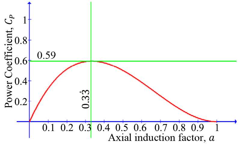
    </mixed-citation>
   </ref>
  </ref-list>
 </back>
</article>