The Corruption Perception Index (CPI) ( Clark, 2018 ; Index, 2018 ) was created in 1995 to gauge public sector corruption perceptions in different countries worldwide. Transparency International (TI) developed a method that involved selecting reliable data sources, standardizing the data, aggregating the re-scaled data, and reporting a measure of uncertainty. Using this approach, TI gathered data from various global sources for 175 countries, categorizing the world into six regions. Data from the World Bank (WB) was also utilized as a credible source for the corruption index ( Kaufmann et al., 2010 ).

In this study of parametric analysis of Corruption Perception Index (CPI) scores, we have established the official mathematical setup and formulation of the probability distribution function (PDF) of the data. Then we have tested the statistical significance for the found PDFs using Kolmogorov-Smirnov test ( Massey Jr., 1951 ), Anderson-Darling ( Anderson & Darling, 1954 ), and χ² goodness-of-fit test ( Cochran, 1952 ) suggested by Prof. Christopher P. Tsokos ( Tsokos, 1972 ) when anyone identifies the PDF of any data-set. The purpose of following this statistical parametric analysis technique is to provide the readers an academic pathway of practicing the process of determination of probability distribution function for special or use case data relevant to the subject matter. In this study, we will be utilizing a data-set gathered by Transparency International, which includes information from 175 countries worldwide. Our goal is to analyze the CPI scores computed by Transparency International and then determine the probability distribution function (PDF) to describe the overall distribution of the CPI scores across the 175 countries. We have identified both the theoretical probability distributions as well as estimated the maximum likelihood estimates of the parameters relevant to each of the identified p.d.f. In this study, we have presented these processes in the following sections in setup where we will present the theoretical p.d.f.s, analytical structures of these p.d.f.s, and then we will present the estimates of the parameters in a table.

We have found that, the best fitted distribution is the “Mixture of 4-Gaussian PDF” data as the initial shape of the histogram showed in Figure 1 . The statistical significance test results given in Table 1 validate our finding as well. Thus, we proceeded with the fitted Mixture of 4-Gaussian p.d.f. of the CPI scores of 175 countries of the world.

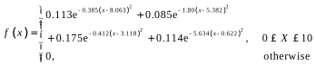
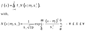
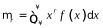
Upon conducting three goodness-of-fit tests, it was determined that the probability distribution of CPI scores conforms to a 4-Mixed Gaussian probability density function (PDF) as shown in Figure 1 . The Gaussian mixture model ( Reynolds, 2009 ) is characterized by two sets of values: the mixture component weights and the component means and variances/covariance. In the case of CPI scores, a Gaussian mixture model with 4 components is utilized, with each component having a mean () and standard deviation () for the univariate case. The analytical structure is represented by Equation (1) for the CPI probability density function.

(1)

Here, .

The r^th moment can be found by

(2)

From Equation (2) anyone can calculate the first four significant moments of the p.d.f.

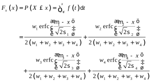
The cumulative distribution function of the CPI scores is given in Equation (3) below:

(3)

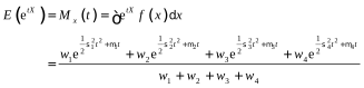
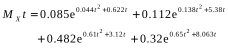
Furthermore, the moment generating function of 1 is given by

(4)

In the following section, we have presented the estimated m.l.e.s of the identified p.d.f either in a table or in an analytical form of the relevant function.

From Table 2 , we see that the mean of the overall CPI scors is 4.73 and median is 4.313 and this data is slightly right skewed with a value of 0.249.

The mean and the variance are 4.75 and 7.34, respectively, with standard deviation of 2.71. For our data, the approximate maximum likelihood estimates (MLEs) of the parameters (, , and , here, ) of 1 are given in the following Table 3 :

Table 3

MLEs of CPI scores
9.18	0.454	5.6	0.67	2.93	1.46	7.54	0.442

Thus, the estimated analytical form of the subject PDF is given by

(5)

In a similar method, we have presented the moment generating function (6) of the identified p.d.f of CPI scores with its estimated parameter values from the data.

(6)

The graph of the p.d.f. give in Equation (5) is given below in Figure 2 .

Suppose a country is chosen randomly from the 175 countries. In this scenario, one can determine the probability of the country falling into one of four corruption categories. Figure 2 displays the Cumulative Distribution Function (c.d.f) of CPI scores. This graph is valuable for calculating the likelihood of a country having a CPI score below a certain threshold. For instance, the probability of a country having a CPI score less than 3.82 is approximately 44%. Furthermore, if we are interested in the probability of a country having a CPI score less than or equal to 7.63, Figure 2 shows that this probability is around 79%. Equation (6) provides the Moment Generating Function (MGF) that can be used to calculate higher order moments and, consequently, the mean and variance of the Mixed Gaussian PDF. When a country is randomly selected from the 175 countries, the expected CPI score is 4.86. The calculated variance is and the standard deviation is . These estimates closely match the basic statistics given in Table 2 , indicating the quality of the fit of the Mixed 4-Gaussian PDF.

In the upcoming sections, we will delve into the procedure for determining the Probability Density Function (PDF) for each of the four categories (represented by the 4 peaks of the histogram of CPI scores shown in Figure 1 ) of the 175 countries in the world.

After performing three goodness-of-fit tests on the current data related to the Least corrupted countries, it has been determined that the data adheres to a distribution called “Mixed of 3-Gaussian PDF.” This distribution has been confirmed by three different methods of goodness-of-fit, as outlined in Table 4 .

Thus, the fitted theoretical PDF of the CPI scores of “Least Corrupted Countries” is given by

(7)

The cumulative distribution function of the CPI scores of Least Corrupted countries of the world is given by

(8)

The estimated m.l.e.s of the parameters that drive the estimated 3-Mixed Gaussian PDF are given in Table 5 below:

Table 5

MLEs of Least Corrupted Countries
8.1	0.32	8.84	0.033	9.51	0.211

With the weights , , and having values 0.43, 0.18, and 0.39 respectively where . So, the analytical structure of the estimated PDF is given by

(9)

The graph of the PDF of Equation (9) is given by Figure 4 below:

The information provided in the graph referenced in Figure 4 can be very helpful for calculating the probability of a randomly selected country from this subset of the population having a score greater than 9. In the graph, the probability of a country having a score more than 9 (i.e. ) is approximately 0.42, as indicated in the same figure.

Figure 5 can be utilized to find the same probability for interested readers and scholars.

This specific portion of the data is somewhat skewed to the left with a value of 0.785, and it has an average of 7.038. The graph displaying the distribution of Fairly Corrupted Countries is shown below in Figure 6 . Based on the graph, it seems like we will need to use a left-skewed probability density function to model this data.

Based on the three goodness-of-fit tests applied to the current data of moderately corrupt countries, it has been determined that the data exhibits probabilistic behavior characterized by the Gumbel PDF. The selection of this model is supported by the results of the three goodness-of-fit methods presented in Table 6 . These results confirm that the most suitable probability density function for the data related to moderately corrupt countries is the Gumbel distribution.

Thus, the fitted theoretical PDF of the subject data is given by

(10)

The c.d.f. of the CPI of Fairly corrupt countries of the world is given by

(11)

The following Table 7 shows the estimated m.l.e.s of the parameters presented in Equation (10). Based on the estimated values of the table, (this is shown in these studies ( Bashar & Tsokos, 2019a, 2019b, 2017 ; Bashar, 2019 )) we have presented the p.d.f. in Equation (12). These values of the m.l.e.s of the parameters of the identified p.d.f. of subset of the CPI scores categorized as Fairly Corrupted countries are given in Table 7 below.

Table 7

MLEs of Fairly Corrupted Countries CPI scores
7.237	0.319

So, the analytical form of the PDF of Fairly corrupted countries of the world is given as follows:

(12)

The graph of the PDF of Equation (12) is given in Figure 7 below.

The mean and standard deviation of the least corrupted data subset are 7.038 and 0.199, respectively. This means that if a country is chosen at random from this subset, we anticipate its CPI score to be around 7.038. Moreover, the likelihood of a country having a CPI score between 6.5 and 7 is 0.283, as indicated in Figure 7 . Its graph of the cumulative distribution function is given in Figure 7 below:

You can use Figure 8 to calculate the probability of a randomly selected country from this population subset scoring between 6.8 and 7.4. This can be computed as the difference between the probabilities of the score being less than or equal to 7.4 and 6.8, which amounts to 0.55.

The analysis of the subset of the overall CPI scores’ categorized as Moderate corrupted countries data using three goodness-of-fit tests indicates that the data exhibits probabilistic behavior described by the Weibull probability density function (PDF). The selection of the Weibull PDF is justified by the results of the three goodness-of-fit tests presented in Table 9 . These results confirm that the Weibull 3-P probability density function is the best fit for the data from Fairly Corrupted countries.

Thus, the fitted theoretical PDF of the subset of the CPI scores data is given by-

(13)

The cumulative distribution function of the Moderately Corrupted Countries of the world is given by

(14)

The MLEs of this PDF of Equation (13) are given in the following Table 10 .

Table 10

MLEs of the Moderately Corrupted Countries
1.938	1.41	3.64

The analytical form of this p.d.f. with estimated parameters is given as follows:

(15)

The cumulative distribution function of the Moderately corrupted country CPI scores with the estimated MLEs of , , and $\hat{\gamma }$ is given below:

$F\left(x\right)=\{\begin{array}{ll}P\left(X\le x\right)=1-{\text{e}}^{-0.544{\left(x-3.65\right)}^{1.82}},\hfill & 3.65<X\hfill \\ 1,\hfill & X>7.62\hfill \end{array}$(16)

The mean and standard deviation of the data subset for moderately corrupted countries are 4.89 and 0.499 respectively. This implies that if a country is chosen randomly from this group, the anticipated CPI score would be around 4.89. Moreover, the likelihood of a country having a CPI score between 4.5 and 5.5 is 0.478, illustrated in Figure 10 . The graph representing the Probability Density Function (PDF) described in Equation (15) can be observed in Figure 10 below.

The method of plotting shown in Figure 11 is especially helpful for calculating the probability of randomly selecting a country from this specific population subset and determining the likelihood of that country scoring between 5 and 5.5 (i.e. $P\left(5\le X\le 5.5\right)$), which is 0.20 according to the subset data.

When applying three goodness-of-fit tests to identify the most suitable candidate for representing the highly corrupted data subset, it was determined that the Johnson SB (4p) ( Parresol, 2003 ) probability density function accurately portrayed the probabilistic characteristics of the highly corrupted data subset. This fact was further confirmed by the goodness-of-fit tests, as shown in Table 12 below:

The analytical structure of the Johnson SB (4p) is given by Equation (17) below:

$f\left(x\right)=\{\begin{array}{ll}\frac{\delta \sigma {\text{e}}^{-\frac{1}{2}{\left(\gamma +\delta \log \left(\frac{x-\mu }{\mu +\sigma -x}\right)\right)}^2}}{\sqrt{2\pi }\left(x-\mu \right)\left(\mu +\sigma -x\right)},\hfill & \mu <x<\mu +\sigma \hfill \\ 0,\hfill & \text{otherwise}\hfill \end{array}$(17)

The estimated MLEs (maximum likelihood estimates) for PDF in Equation (17) are given in the following Table 13 :

The fitted PDF with estimated parameters is given by Equation (18) below:

$f\left(x\right)=\{\begin{array}{ll}\frac{0.82{\text{e}}^{-\frac{1}{2}{\left(0.55\log \left(\frac{x-0.029}{3.741-x}\right)-0.36\right)}^2}}{\left(x-0.029\right)\left(3.741-x\right)},\hfill & \text{if}0<X<3.65\hfill \\ 0,\hfill & \text{Otherwise}\hfill \end{array}$(18)

The cumulative distribution function is given by

$\begin{array}{c}F\left(x\right)=P\left(X\le x\right)\\ =\{\begin{array}{ll}\frac{1}{2}\text{erfc}\left(-\frac{0.552\log \left(\frac{x-0.029}{3.74-x}\right)-0.36}{\sqrt{2}}\right),\hfill & 0.03<x<1.88\hfill \\ \frac{1}{2}\left(\text{erf}\left(\frac{0.552\log \left(\frac{x-0.029}{3.74-x}\right)-0.36}{\sqrt{2}}\right)+1\right),\hfill & 1.88\le x<3.74\hfill \\ 1,\hfill & x\ge 3.74\hfill \end{array}\end{array}$(19)

The graph of the PDF of Equation (18) is given in Figure 13 .

The mean and variance of the subset of country data with high levels of corruption are 2.273 and 1.1648, respectively. This means that if a country is randomly chosen from this group, we anticipate its CPI score to be around 2.3. Moreover, the likelihood of a country having a CPI score between 2 and 3 is 0.273, as illustrated in Figure 14 . The CDF plot of the Equation (19) is given below:

The information presented in Figure 14 can be valuable for determining the likelihood of a randomly selected country from a specific population subset having a score between 2 and 2.5. The probability of this occurrence, represented as $P\left(2\le X\le 3\right)$, is 0.27.