<?xml version="1.0" encoding="UTF-8"?><!DOCTYPE article PUBLIC "-//NLM//DTD Journal Publishing DTD v3.0 20080202//EN" "http://dtd.nlm.nih.gov/publishing/3.0/journalpublishing3.dtd">
<article xmlns:mml="http://www.w3.org/1998/Math/MathML" xmlns:xlink="http://www.w3.org/1999/xlink" dtd-version="3.0" xml:lang="en" article-type="research article">
 <front>
  <journal-meta>
   <journal-id journal-id-type="publisher-id">
    jmp
   </journal-id>
   <journal-title-group>
    <journal-title>
     Journal of Modern Physics
    </journal-title>
   </journal-title-group>
   <issn pub-type="epub">
    2153-1196
   </issn>
   <issn publication-format="print">
    2153-120X
   </issn>
   <publisher>
    <publisher-name>
     Scientific Research Publishing
    </publisher-name>
   </publisher>
  </journal-meta>
  <article-meta>
   <article-id pub-id-type="doi">
    10.4236/jmp.2024.158048
   </article-id>
   <article-id pub-id-type="publisher-id">
    jmp-134528
   </article-id>
   <article-categories>
    <subj-group subj-group-type="heading">
     <subject>
      Articles
     </subject>
    </subj-group>
    <subj-group subj-group-type="Discipline-v2">
     <subject>
      Physics 
     </subject>
     <subject>
       Mathematics
     </subject>
    </subj-group>
   </article-categories>
   <title-group>
    Extinction of Light in the Galactic Halo: First Observational Evidence of the Interaction of Light and Dark Matter
   </title-group>
   <contrib-group>
    <contrib contrib-type="author" xlink:type="simple">
     <name name-style="western">
      <surname>
       Charles H. McGruder
      </surname>
      <given-names>
       III
      </given-names>
     </name>
    </contrib>
   </contrib-group> 
   <aff id="affnull">
    <addr-line>
     aDepartment of Physics and Astronomy, Western Kentucky University, Bowling Green, USA
    </addr-line> 
   </aff> 
   <pub-date pub-type="epub">
    <day>
     11
    </day> 
    <month>
     07
    </month>
    <year>
     2024
    </year>
   </pub-date> 
   <volume>
    15
   </volume> 
   <issue>
    08
   </issue>
   <fpage>
    1144
   </fpage>
   <lpage>
    1198
   </lpage>
   <history>
    <date date-type="received">
     <day>
      22,
     </day>
     <month>
      March
     </month>
     <year>
      2024
     </year>
    </date>
    <date date-type="published">
     <day>
      13,
     </day>
     <month>
      March
     </month>
     <year>
      2024
     </year> 
    </date> 
    <date date-type="accepted">
     <day>
      13,
     </day>
     <month>
      July
     </month>
     <year>
      2024
     </year> 
    </date>
   </history>
   <permissions>
    <copyright-statement>
     © Copyright 2014 by authors and Scientific Research Publishing Inc. 
    </copyright-statement>
    <copyright-year>
     2014
    </copyright-year>
    <license>
     <license-p>
      This work is licensed under the Creative Commons Attribution International License (CC BY). http://creativecommons.org/licenses/by/4.0/
     </license-p>
    </license>
   </permissions>
   <abstract>
    We study the distribution of quasars on the celestial sphere according to ground-based SDSS and space-based WISE and Gaia observations. All distributions as a function of galactic latitude, b, exhibit a decrease in quasar frequency well outside the dust in and near the galactic plane. We prove that the observed decrease in quasar frequency at high galactic latitudes is not accompanied by reddening, meaning that it can not be caused by dust. The scattering of light by the circumgalactic gas is negligible because the Thomson scattering cross section is very small. We conclude the observed scattering of light must be caused by dark matter in the galactic halo. We determine the mass and charge of dark matter particles. If the dark matter particle is a fermion its mass, 
    <math display="inline" xmlns="http://www.w3.org/1998/Math/MathML"> <mrow> 
      <msub> 
       <mi>
        m
       </mi> 
       <mrow> 
        <mi>
         D
        </mi>
        <mi>
         M
        </mi>
       </mrow> 
      </msub> 
     </mrow> 
    </math> and charge 
    <math display="inline" xmlns="http://www.w3.org/1998/Math/MathML"> <mrow> 
      <msub> 
       <mi>
        e
       </mi> 
       <mrow> 
        <mi>
         D
        </mi>
        <mi>
         M
        </mi>
       </mrow> 
      </msub> 
      <mo>
       =
      </mo>
      <mi>
       δ
      </mi>
      <mi>
       e
      </mi>
     </mrow> 
    </math> , where e is the elementary charge are: 
    <math display="inline" xmlns="http://www.w3.org/1998/Math/MathML"> <mrow> 
      <msub> 
       <mi>
        m
       </mi> 
       <mrow> 
        <mi>
         D
        </mi>
        <mi>
         M
        </mi>
       </mrow> 
      </msub> 
      <mo>
       =
      </mo>
      <mn>
       3.2
      </mn>
      <mo>
       ×
      </mo>
      <msup> 
       <mrow> 
        <mn>
         10
        </mn>
       </mrow> 
       <mrow> 
        <mo>
         −
        </mo>
        <mn>
         2
        </mn>
       </mrow> 
      </msup> 
     </mrow> 
    </math> eV and 
    <math display="inline" xmlns="http://www.w3.org/1998/Math/MathML"> <mrow> 
      <mi>
       δ
      </mi>
      <mo>
       =
      </mo>
      <mn>
       3.856
      </mn>
      <mo>
       ×
      </mo>
      <msup> 
       <mrow> 
        <mn>
         10
        </mn>
       </mrow> 
       <mrow> 
        <mo>
         −
        </mo>
        <mn>
         5
        </mn>
       </mrow> 
      </msup> 
     </mrow> 
    </math> . If however the dark matter particle is spinless then: 
    <math display="inline" xmlns="http://www.w3.org/1998/Math/MathML"> <mrow> 
      <msub> 
       <mi>
        m
       </mi> 
       <mrow> 
        <mi>
         D
        </mi>
        <mi>
         M
        </mi>
       </mrow> 
      </msub> 
      <mo>
       =
      </mo>
      <mn>
       0.511
      </mn>
     </mrow> 
    </math> eV and 
    <math display="inline" xmlns="http://www.w3.org/1998/Math/MathML"> <mrow> 
      <mi>
       δ
      </mi>
      <mo>
       =
      </mo>
      <mn>
       2.132
      </mn>
      <mo>
       ×
      </mo>
      <msup> 
       <mrow> 
        <mn>
         10
        </mn>
       </mrow> 
       <mrow> 
        <mo>
         −
        </mo>
        <mn>
         4
        </mn>
       </mrow> 
      </msup> 
     </mrow> 
    </math> . These values for the charge of a dark matter particle are orders of magnitude higher than the upper limit of the neutrino charge according to laboratory experiments. Consequently, dark matter particles are not charged neutrinos. Since dark matter particles are charged, they must emit and absorb electromagnetic radiation. However, 
    <math display="inline" xmlns="http://www.w3.org/1998/Math/MathML"> <mrow> 
      <msub> 
       <mi>
        P
       </mi> 
       <mrow> 
        <mi>
         D
        </mi>
        <mi>
         M
        </mi>
       </mrow> 
      </msub> 
      <mo>
       ~
      </mo>
      <msup> 
       <mi>
        δ
       </mi> 
       <mn>
        2
       </mn> 
      </msup> 
     </mrow> 
    </math> , or: 
    <math display="inline" xmlns="http://www.w3.org/1998/Math/MathML"> <mrow> 
      <msub> 
       <mi>
        P
       </mi> 
       <mrow> 
        <mi>
         D
        </mi>
        <mi>
         M
        </mi>
       </mrow> 
      </msub> 
      <mo>
       ~
      </mo>
      <mn>
       1.487
      </mn>
      <mo>
       ×
      </mo>
      <msup> 
       <mrow> 
        <mn>
         10
        </mn>
       </mrow> 
       <mrow> 
        <mo>
         −
        </mo>
        <mn>
         9
        </mn>
       </mrow> 
      </msup> 
      <msub> 
       <mi>
        P
       </mi> 
       <mi>
        e
       </mi> 
      </msub> 
     </mrow> 
    </math> , where 
    <math display="inline" xmlns="http://www.w3.org/1998/Math/MathML"> <mrow> 
      <msub> 
       <mi>
        P
       </mi> 
       <mi>
        e
       </mi> 
      </msub> 
     </mrow> 
    </math> is the power output of a single electron.
   </abstract>
   <kwd-group> 
    <kwd>
     Milky Way Dark Matter Halo (1049)
    </kwd>
   </kwd-group>
  </article-meta>
 </front>
 <body>
  <sec id="s1">
   <title>1. Introduction</title>
   <p>This work has three primary objectives: 1) to determine why the observed distribution of quasars on the celestial sphere is highly anisotropic, 2) to demonstrate that the extinction of light is taking place in the halo of the Milky Way, and 3) to ascertain what component of the galactic halo is the cause of the observed extinction.</p>
   <p>Our results are based on the following observations and assumptions: 1) the observed distribution of quasars as a function of galactic latitude, b. 2) The assumption that quasars are distributed homogeneously in space. 3) The galactic halo contains only stars, hot plasma, dark matter and dust. 4) We provisionally assume that dark matter neither absorbs nor emits light.</p>
   <p>Our approach to accomplish our three primary objectives is to first develop a theoretical expression, which allows us to compute the expected isotropic distribution of quasars. We then compare the theoretical isotropic distributions with observations of the distribution of quasars on the celestial sphere, which are highly anisotropic. We conclude that the discrepancy between theory and observation is caused by the extinction of quasar light. We then investigate a number of circumstances, which could possibly cause the extinction.</p>
   <p>Extinction consists of absorption plus scattering of light. All observational evidence to date, suggests that dark matter neither absorbs nor emits light. So what happens when visible photons collide with dark matter particles? Below we present evidence that the light is scattered, that is, it is responsible for the observed extinction of quasar light.</p>
   <p>It is known that matter in local spaces of the universe is not homogeneously distributed. It occurs in spatially limited structural units—galaxies, clusters of galaxies and superclusters, which are separated by voids. It is however thought that if one considers large spaces with redshift, 
    <math display="inline" xmlns="http://www.w3.org/1998/Math/MathML"> <mrow> 
      <mi>
        z 
      </mi> 
      <mo>
        &gt; 
      </mo> 
      <mn>
        0.2 
      </mn> 
     </mrow> 
    </math>, then the matter in the universe is homogeneously distributed. However, it is difficult to confirm homogeneity because there are very few types of celestial sources that can be detected at such distances. One type that can be is quasars.</p>
   <p>Gattano et al. <xref ref-type="bibr" rid="scirp.134528-1">
     [1]
    </xref> found that quasars appear not to be isotropically distributed on the celestial sphere. This result was obtained by dividing their data into rather large intervals of 10˚. They explicitly noted that their results were chiefly based on ground-based data that are severely limited by the lack of observations from the southern hemisphere. In our study of the distribution of quasars on the celestial sphere, we use much larger data sets, which allows us to divide the data into intervals of 0.1˚. In addition to ground-based observations from SDSS we also analyze space-based observations from both the WISE and Gaia spacecraft. The space-based data shows that the observed distribution of quasars on the celestial sphere is highly anisotropic.</p>
   <p>However, one of the basic assumptions that standard cosmological theory is based on is: The matter in the universe is homogeneously distributed. If this assumption can be shown to be incorrect, then the current widely accepted theory of cosmology must be revised or even discarded. Thus, it is crucially important that it be demonstrated that this assumption is indeed correct.</p>
   <p>We see that theory demands that quasars be distributed is otropically on the celestial sphere, whereas observations show they are not. How are we going to resolve this discrepancy between theory and observations? To make clear our answer to this question, we present a well known historical analogy. In the geocentric theory the assumption is made that the observed daily solar motion across the sky is real. Aristarchus of Samos however maintained in his heliocentric theory that the observed diurnal solar motion is apparent motion caused by the rotation of the earth. Similarly, we show below that the observed anisotropic distribution of quasars on the celestial sphere is apparent and does not correspond to the real homogeneous distribution that one would observe from intergalactic space. What then is the cause of the apparent anisotropic distribution of quasars that is actually observed? The extinction of quasar light in the galactic halo, which distorts the original isotropic distribution.</p>
   <p>The above shows that the main topics touched on in our investigation are: Galactic extinction, the spatial distribution of quasars and the cosmological principle, which asserts that the matter in the universe is homogeneously and isotropically distributed on large scales. In addition our investigation will involve the question of whether alternate gravitational theories, that are employed to explain many of the phenomenon associated with dark matter, are tenable. Finally, our work concerns dark matter particles, specifically the scattering of light by dark matter particles.</p>
   <p>Extinction in the Milky Way has been studied extensively by Green et al. <xref ref-type="bibr" rid="scirp.134528-2">
     [2]
    </xref>. Previously, Schlegel et al. <xref ref-type="bibr" rid="scirp.134528-3">
     [3]
    </xref> created two-dimensional maps of reddening due to dust. Their work was followed by a number of authors, who improved the high galactic latitude portion, namely: York et al. <xref ref-type="bibr" rid="scirp.134528-4">
     [4]
    </xref>, Schlafly et al. <xref ref-type="bibr" rid="scirp.134528-5">
     [5]
    </xref>, Peek &amp; Graves <xref ref-type="bibr" rid="scirp.134528-6">
     [6]
    </xref>, Jones et al. <xref ref-type="bibr" rid="scirp.134528-7">
     [7]
    </xref>, Schlafly &amp; Finkbeiner <xref ref-type="bibr" rid="scirp.134528-8">
     [8]
    </xref>, Peek &amp; Schiminovich <xref ref-type="bibr" rid="scirp.134528-9">
     [9]
    </xref>, Yuan et al. <xref ref-type="bibr" rid="scirp.134528-10">
     [10]
    </xref> and Wang &amp; Jiang <xref ref-type="bibr" rid="scirp.134528-11">
     [11]
    </xref>. In addition Pelgrims <xref ref-type="bibr" rid="scirp.134528-12">
     [12]
    </xref> has investigated the influence of Galactic dust on the polarization of quasar radiation. The extinction considered by these authors is caused by Galactic dust, which is always accompanied by reddening. Below we show that the observed extinction of quasar light is not caused by dust.</p>
   <p>The spatial distribution of quasars has been investigated by Pâris et al. <xref ref-type="bibr" rid="scirp.134528-13">
     [13]
    </xref>, Gattano et al. <xref ref-type="bibr" rid="scirp.134528-1">
     [1]
    </xref>, Pilipenko <xref ref-type="bibr" rid="scirp.134528-14">
     [14]
    </xref> and Dravskikh &amp; Dravskikh <xref ref-type="bibr" rid="scirp.134528-15">
     [15]
    </xref>. Hartwick &amp; Schade <xref ref-type="bibr" rid="scirp.134528-16">
     [16]
    </xref> reviewed the space distribution of quasars and Arp <xref ref-type="bibr" rid="scirp.134528-17">
     [17]
    </xref> pointed out that bright quasars are concentrated in the direction of the local group.</p>
   <p>The cosmological principle has been discussed by Zhao &amp; Santo <xref ref-type="bibr" rid="scirp.134528-18">
     [18]
    </xref>, who found that angular anomalies in cosmological data are not due to a violation of the cosmological principle, but appear to be associated with the motion of our local group of galaxies relative to the cosmic microwave background. Marocco &amp; Eisenhardt <xref ref-type="bibr" rid="scirp.134528-19">
     [19]
    </xref> found that the galaxy distribution, as traced by luminous red galaxies, appears to be isotropic to every comoving observer in the universe if the averaging scale is larger than a specific value. Maartens <xref ref-type="bibr" rid="scirp.134528-20">
     [20]
    </xref> emphasizes that homogeneity cannot be confirmed via observations because all astronomical data is light-cone based, whereas isotropy can be confirmed by observations. Observationally, Pelgrims <xref ref-type="bibr" rid="scirp.134528-21">
     [21]
    </xref> argues that the polarization of quasar radiation can be employed to explore the validity of the isotropic principle. In our investigation we do not contribute to the discussion of the cosmological principle, homogeneity and isotropy rather instead we assume their validity.</p>
   <p>The existence or reality of dark matter has been debated for many decades. For a review see: Bertone &amp; Tait <xref ref-type="bibr" rid="scirp.134528-22">
     [22]
    </xref>. Alternative gravitational theories, which do not invoke the existence of dark matter, have successfully explained many of the gravitational effects commonly associated with dark matter (Milgrom <xref ref-type="bibr" rid="scirp.134528-23">
     [23]
    </xref>, Miller &amp; Bregman <xref ref-type="bibr" rid="scirp.134528-24">
     [24]
    </xref>, Moffat <xref ref-type="bibr" rid="scirp.134528-25">
     [25]
    </xref>, Brownstein &amp; Moffat <xref ref-type="bibr" rid="scirp.134528-26">
     [26]
    </xref>, Ghaffarnejad &amp; Dehghani <xref ref-type="bibr" rid="scirp.134528-27">
     [27]
    </xref>, Milgrom <xref ref-type="bibr" rid="scirp.134528-23">
     [23]
    </xref> <xref ref-type="bibr" rid="scirp.134528-28">
     [28]
    </xref>). In particular they explain the rotational curves of hundreds of spiral galaxies and the Tully-Fisher relationship between the luminosity and rotational velocity of spiral galaxies. The most successful relativistic alternative gravitational theory was published by Bekenstein <xref ref-type="bibr" rid="scirp.134528-29">
     [29]
    </xref>. It is commonly referred to as the Tensor-Vector-Scalar (TeVeS) theory. TeVeS appears to successfully explain gravitational lensing and specific cosmological problems such as structure formation and the cosmological microwave background.</p>
   <p>Kroupa <xref ref-type="bibr" rid="scirp.134528-30">
     [30]
    </xref> <xref ref-type="bibr" rid="scirp.134528-31">
     [31]
    </xref> and Kroupa et al. <xref ref-type="bibr" rid="scirp.134528-32">
     [32]
    </xref> pointed out that a number of observational tests contradict the standard cosmological model, which assumes the existence of dark matter. In 2016 two papers were published which gave strong support to alternative gravitational theories. López-Corredoira &amp; Kroupa <xref ref-type="bibr" rid="scirp.134528-33">
     [33]
    </xref> found a correlation between the number of tidal dwarf satellite galaxies as a function of the bulge index in agreement with alternative gravitational theories and in disagreement with the prediction of dark matter theory. McGaugh et al. <xref ref-type="bibr" rid="scirp.134528-34">
     [34]
    </xref> found a strong correlation between the radial acceleration associated with rotation curves and the observed distribution of baryonic mass without invoking the existence of dark matter.</p>
   <p>In general alternative gravitational theories are chiefly viable because of the failure to detect dark matter particles in the laboratory despite decades of effort with over twenty experiments (Bekenstein <xref ref-type="bibr" rid="scirp.134528-29">
     [29]
    </xref>, Graham et al. <xref ref-type="bibr" rid="scirp.134528-35">
     [35]
    </xref>, Kamaha <xref ref-type="bibr" rid="scirp.134528-36">
     [36]
    </xref>, Undagoitia &amp; Rauch <xref ref-type="bibr" rid="scirp.134528-37">
     [37]
    </xref>, Irastorza &amp; Redondo <xref ref-type="bibr" rid="scirp.134528-38">
     [38]
    </xref>, Schumann <xref ref-type="bibr" rid="scirp.134528-39">
     [39]
    </xref>, Heros <xref ref-type="bibr" rid="scirp.134528-40">
     [40]
    </xref>). Alternative gravitational theories explain this failure by simply maintaining that dark matter does not exist. Our investigation contributes to this debate in that it presents observational data, which indicates that dark matter scatters light.</p>
   <p>In the literature Bertone et al. <xref ref-type="bibr" rid="scirp.134528-41">
     [41]
    </xref>, Bertone &amp; Hooper <xref ref-type="bibr" rid="scirp.134528-42">
     [42]
    </xref>, Bertone &amp; Tait <xref ref-type="bibr" rid="scirp.134528-22">
     [22]
    </xref> many non-baryonic dark matter candidates are being or have been discussed: Standard model axions (Safarzadeh &amp; Spergel <xref ref-type="bibr" rid="scirp.134528-43">
     [43]
    </xref>, Glennon et al. <xref ref-type="bibr" rid="scirp.134528-44">
     [44]
    </xref>), neutrinos and sterile neutrinos. In addition there are the supersymmetric candidates: Neutralinos, Sneutrinos, Gravitinos and Axinos. We have mentioned only some of the most popular candidates. There are many more candidates. Today, however, the leading class of dark matter candidates is weakly interacting massive particles, WIMPs, Arcadi et al. <xref ref-type="bibr" rid="scirp.134528-45">
     [45]
    </xref>. Most of these dark matter candidates have in common is that they do not participate in the electromagnetic interaction. However, it has been suggested that they may be mini-charged dark matter (Alexander et al. <xref ref-type="bibr" rid="scirp.134528-46">
     [46]
    </xref>, Cline et al. <xref ref-type="bibr" rid="scirp.134528-47">
     [47]
    </xref>, Munoz &amp; Loeb <xref ref-type="bibr" rid="scirp.134528-48">
     [48]
    </xref>). In this work we attempt to answer some of the fundamental questions associated with dark matter particles: What are their charge, mass and spin?</p>
   <p>Even though to date the scattering of light by dark matter particles has not been demonstrated, nevertheless the hypothetical non-zero photon-dark matter cross section has been discussed by Cline et al. <xref ref-type="bibr" rid="scirp.134528-47">
     [47]
    </xref>, Davis &amp; Silk <xref ref-type="bibr" rid="scirp.134528-49">
     [49]
    </xref>, Wilkinson et al. <xref ref-type="bibr" rid="scirp.134528-50">
     [50]
    </xref>, McDermott et al. <xref ref-type="bibr" rid="scirp.134528-51">
     [51]
    </xref> and Foot &amp; Volkas <xref ref-type="bibr" rid="scirp.134528-52">
     [52]
    </xref>. Below we present the first observational evidence of the interaction of dark matter and light.</p>
  </sec><sec id="s2">
   <title>2. Theory</title>
   <p>The assumption that matter in the universe is distributed homogeneously means that it must also be isotropically distributed. Thus, independent of the direction we observe, we should see the same number of quasars/deg<sup>2</sup>. We will derive a mathematical expression in spherical coordinates, which expresses this circumstance. But, first we start with a more general expression, which assumes that quasars are anisotropically distributed on the celestial sphere. From the well-known expression for the differential surface area on a sphere it is clear that the differential number of quasars, dn, on the celestial sphere is given by:</p>
   <p>
    <math display="inline" xmlns="http://www.w3.org/1998/Math/MathML"> <mrow> 
      <mtext>
        d 
      </mtext> 
      <mi>
        n 
      </mi> 
      <mo>
        = 
      </mo> 
      <mi>
        ζ 
      </mi> 
      <mrow> 
       <mo>
         ( 
       </mo> 
       <mrow> 
        <mi>
          μ 
        </mi> 
        <mo>
          , 
        </mo> 
        <mi>
          ν 
        </mi> 
       </mrow> 
       <mo>
         ) 
       </mo> 
      </mrow> 
      <mfrac> 
       <mi>
         n 
       </mi> 
       <mrow> 
        <mn>
          4 
        </mn> 
        <mi>
          π 
        </mi> 
       </mrow> 
      </mfrac> 
      <mi>
        sin 
      </mi> 
      <mrow> 
       <mo>
         ( 
       </mo> 
       <mi>
         μ 
       </mi> 
       <mo>
         ) 
       </mo> 
      </mrow> 
      <mtext>
        d 
      </mtext> 
      <mi>
        μ 
      </mi> 
      <mtext>
        d 
      </mtext> 
      <mi>
        ν 
      </mi> 
      <mo>
        , 
      </mo> 
     </mrow> 
    </math>(1)</p>
   <p>where μ is the polar angle and ν, the azimuthal angle. Integration over the entire sphere gives n, which is the total number of quasars in the sample. Equation (1) applies to the general case of an anisotropic distribution. The anisotropy is described mathematically via the function, 
    <math display="inline" xmlns="http://www.w3.org/1998/Math/MathML"> <mrow> 
      <mi>
        ζ 
      </mi> 
      <mrow> 
       <mo>
         ( 
       </mo> 
       <mrow> 
        <mi>
          μ 
        </mi> 
        <mo>
          , 
        </mo> 
        <mi>
          ν 
        </mi> 
       </mrow> 
       <mo>
         ) 
       </mo> 
      </mrow> 
     </mrow> 
    </math>. The special case of a homogeneous distribution is given when 
    <math display="inline" xmlns="http://www.w3.org/1998/Math/MathML"> <mrow> 
      <mi>
        ζ 
      </mi> 
      <mrow> 
       <mo>
         ( 
       </mo> 
       <mrow> 
        <mi>
          μ 
        </mi> 
        <mn>
          , 
        </mn> 
        <mi>
          ν 
        </mi> 
       </mrow> 
       <mo>
         ) 
       </mo> 
      </mrow> 
      <mo>
        = 
      </mo> 
      <mn>
        1 
      </mn> 
     </mrow> 
    </math>. In this case Equation (1) becomes:</p>
   <p>
    <math display="inline" xmlns="http://www.w3.org/1998/Math/MathML"> <mrow> 
      <mtext>
        d 
      </mtext> 
      <mi>
        n 
      </mi> 
      <mo>
        = 
      </mo> 
      <mfrac> 
       <mi>
         n 
       </mi> 
       <mrow> 
        <mn>
          4 
        </mn> 
        <mi>
          π 
        </mi> 
       </mrow> 
      </mfrac> 
      <mi>
        sin 
      </mi> 
      <mrow> 
       <mo>
         ( 
       </mo> 
       <mi>
         μ 
       </mi> 
       <mo>
         ) 
       </mo> 
      </mrow> 
      <mtext>
        d 
      </mtext> 
      <mi>
        μ 
      </mi> 
      <mtext>
        d 
      </mtext> 
      <mi>
        ν 
      </mi> 
      <mo>
        . 
      </mo> 
     </mrow> 
    </math>(2)</p>
   <p>We want to compare this differential equation with observations, which are expressed in finite intervals. So we must integrate Equation (2). To facilitate this we introduce two auxiliary quantities, ∆ and m. The first quantity, ∆, is the size of the finite interval, which we set at 0.1˚. The second quantity, m, is an integer. It represents the finite interval under consideration. The polar coordinate possesses the range: 
    <math display="inline" xmlns="http://www.w3.org/1998/Math/MathML"> <mrow> 
      <mo>
        − 
      </mo> 
      <msup> 
       <mrow> 
        <mn>
          90 
        </mn> 
       </mrow> 
       <mo>
         ∘ 
       </mo> 
      </msup> 
      <mo>
        ≤ 
      </mo> 
      <mi>
        μ 
      </mi> 
      <mo>
        ≤ 
      </mo> 
      <msup> 
       <mrow> 
        <mn>
          90 
        </mn> 
       </mrow> 
       <mo>
         ∘ 
       </mo> 
      </msup> 
     </mrow> 
    </math>, so 
    <math display="inline" xmlns="http://www.w3.org/1998/Math/MathML"> <mrow> 
      <mn>
        1 
      </mn> 
      <mo>
        ≤ 
      </mo> 
      <mi>
        m 
      </mi> 
      <mo>
        ≤ 
      </mo> 
      <mn>
        1800 
      </mn> 
     </mrow> 
    </math>. Integration of Equation (2) for the distribution in polar coordinate, μ, yields:</p>
   <p>
    <math display="inline" xmlns="http://www.w3.org/1998/Math/MathML"> <mrow> 
      <mfrac> 
       <mi>
         n 
       </mi> 
       <mrow> 
        <mn>
          4 
        </mn> 
        <mi>
          π 
        </mi> 
       </mrow> 
      </mfrac> 
      <mstyle displaystyle="true"> 
       <mrow> 
        <msubsup> 
         <mo>
           ∫ 
         </mo> 
         <mn>
           0 
         </mn> 
         <mrow> 
          <mn>
            2 
          </mn> 
          <mi>
            π 
          </mi> 
         </mrow> 
        </msubsup> 
       </mrow> 
      </mstyle> 
      <mstyle displaystyle="true"> 
       <mrow> 
        <msubsup> 
         <mo>
           ∫ 
         </mo> 
         <mrow> 
          <mi>
            m 
          </mi> 
          <mi>
            Δ 
          </mi> 
         </mrow> 
         <mrow> 
          <mi>
            m 
          </mi> 
          <mi>
            Δ 
          </mi> 
          <mo>
            + 
          </mo> 
          <mi>
            Δ 
          </mi> 
         </mrow> 
        </msubsup> 
       </mrow> 
      </mstyle> 
      <mi>
        sin 
      </mi> 
      <mrow> 
       <mo>
         ( 
       </mo> 
       <mi>
         μ 
       </mi> 
       <mo>
         ) 
       </mo> 
      </mrow> 
      <mtext>
        d 
      </mtext> 
      <mi>
        μ 
      </mi> 
      <mtext>
        d 
      </mtext> 
      <mi>
        ν 
      </mi> 
      <mo>
        = 
      </mo> 
      <mfrac> 
       <mi>
         n 
       </mi> 
       <mn>
         2 
       </mn> 
      </mfrac> 
      <mi>
        cos 
      </mi> 
      <mrow> 
       <mo>
         ( 
       </mo> 
       <mrow> 
        <mi>
          m 
        </mi> 
        <mi>
          Δ 
        </mi> 
       </mrow> 
       <mo>
         ) 
       </mo> 
      </mrow> 
      <mo>
        − 
      </mo> 
      <mfrac> 
       <mi>
         n 
       </mi> 
       <mn>
         2 
       </mn> 
      </mfrac> 
      <mi>
        cos 
      </mi> 
      <mrow> 
       <mo>
         [ 
       </mo> 
       <mrow> 
        <mrow> 
         <mo>
           ( 
         </mo> 
         <mrow> 
          <mn>
            1 
          </mn> 
          <mo>
            + 
          </mo> 
          <mi>
            m 
          </mi> 
         </mrow> 
         <mo>
           ) 
         </mo> 
        </mrow> 
        <mi>
          Δ 
        </mi> 
       </mrow> 
       <mo>
         ] 
       </mo> 
      </mrow> 
      <mn>
        . 
      </mn> 
     </mrow> 
    </math>(3)</p>
   <p>Summing over all intervals leads to the total number of sources in the dataset:</p>
   <p>
    <math display="inline" xmlns="http://www.w3.org/1998/Math/MathML"> <mrow> 
      <mstyle displaystyle="true"> 
       <munderover> 
        <mo>
          ∑ 
        </mo> 
        <mn>
          1 
        </mn> 
        <mrow> 
         <mn>
           1800 
         </mn> 
        </mrow> 
       </munderover> 
      </mstyle> 
      <mfrac> 
       <mi>
         n 
       </mi> 
       <mn>
         2 
       </mn> 
      </mfrac> 
      <mi>
        cos 
      </mi> 
      <mrow> 
       <mo>
         ( 
       </mo> 
       <mrow> 
        <mi>
          m 
        </mi> 
        <mi>
          Δ 
        </mi> 
       </mrow> 
       <mo>
         ) 
       </mo> 
      </mrow> 
      <mo>
        − 
      </mo> 
      <mfrac> 
       <mi>
         n 
       </mi> 
       <mn>
         2 
       </mn> 
      </mfrac> 
      <mi>
        cos 
      </mi> 
      <mrow> 
       <mo>
         [ 
       </mo> 
       <mrow> 
        <mrow> 
         <mo>
           ( 
         </mo> 
         <mrow> 
          <mn>
            1 
          </mn> 
          <mo>
            + 
          </mo> 
          <mi>
            m 
          </mi> 
         </mrow> 
         <mo>
           ) 
         </mo> 
        </mrow> 
        <mi>
          Δ 
        </mi> 
       </mrow> 
       <mo>
         ] 
       </mo> 
      </mrow> 
      <mo>
        = 
      </mo> 
      <mi>
        n 
      </mi> 
      <mn>
        . 
      </mn> 
     </mrow> 
    </math>(4)</p>
   <p>As an example, the right side of Equation (3) is plotted in <xref ref-type="fig" rid="fig1">
     Figure 1
    </xref> for the</p>
   <fig id="fig1" position="float">
    <label>Figure 1</label>
    <caption>
     <title>Figure 1. Theoretical Quasar Distribution Assuming Homogeneity.</title>
    </caption>
    <graphic mimetype="image" position="float" xlink:type="simple" xlink:href="https://html.scirp.org/file/7505280-rId49.jpeg?20240716105750" />
   </fig>
   <p>case of 
    <math display="inline" xmlns="http://www.w3.org/1998/Math/MathML"> <mrow> 
      <mi>
        n 
      </mi> 
      <mo>
        = 
      </mo> 
      <mn>
        100000 
      </mn> 
     </mrow> 
    </math>. This plot represents the theoretical distribution assuming isotropy and it is independent of the spherical coordinate system employed. If we do not have isotropy, 
    <math display="inline" xmlns="http://www.w3.org/1998/Math/MathML"> <mrow> 
      <mi>
        ζ 
      </mi> 
      <mrow> 
       <mo>
         ( 
       </mo> 
       <mrow> 
        <mi>
          μ 
        </mi> 
        <mn>
          , 
        </mn> 
        <mi>
          ν 
        </mi> 
       </mrow> 
       <mo>
         ) 
       </mo> 
      </mrow> 
      <mo>
        ≠ 
      </mo> 
      <mn>
        1 
      </mn> 
     </mrow> 
    </math>, then 
    <math display="inline" xmlns="http://www.w3.org/1998/Math/MathML"> <mi>
       ζ 
     </mi> 
    </math> will be different in the various spherical coordinate systems. Most importantly, <xref ref-type="fig" rid="fig1">
     Figure 1
    </xref> shows that the beginning and end of the distribution is practically a straight line. We will use this circumstance below to compute the expected theoretical isotropic distributions for the SDSS, WISE and Gaia datasets.</p>
  </sec><sec id="s3">
   <title>3. Observations</title>
   <p>The black filled circles in <xref ref-type="fig" rid="fig2">
     Figure 2
    </xref> show the distribution of the quasars from the Sloan Digital Sky Survey (SDSS) as a function of galactic latitude, b. 
    <math display="inline" xmlns="http://www.w3.org/1998/Math/MathML"> <mrow> 
      <mi>
        n 
      </mi> 
      <mo>
        = 
      </mo> 
      <mn>
        1373629 
      </mn> 
     </mrow> 
    </math> ground-based observations of quasars from SDSS, as compiled in the MILLIQUAS—Million Quasars Catalog, Version 6.2, Flesch <xref ref-type="bibr" rid="scirp.134528-53">
     [53]
    </xref>, which includes SDSS-DR15 (Aguado et al. <xref ref-type="bibr" rid="scirp.134528-54">
     [54]
    </xref>) were used in <xref ref-type="fig" rid="fig2">
     Figure 2
    </xref>. Striking is the lack of quasars around 
    <math display="inline" xmlns="http://www.w3.org/1998/Math/MathML"> <mrow> 
      <mi>
        b 
      </mi> 
      <mo>
        ≈ 
      </mo> 
      <msup> 
       <mn>
         0 
       </mn> 
       <mo>
         ∘ 
       </mo> 
      </msup> 
     </mrow> 
    </math>. This is due to galactic extinction and to the lack of observations in the southern sky. In addition we note that the figure is highly asymmetric relative to 
    <math display="inline" xmlns="http://www.w3.org/1998/Math/MathML"> <mrow> 
      <mi>
        b 
      </mi> 
      <mo>
        = 
      </mo> 
      <msup> 
       <mn>
         0 
       </mn> 
       <mo>
         ∘ 
       </mo> 
      </msup> 
     </mrow> 
    </math>. This is due to the paucity of observations in the southern sky. Finally, we note that the number of quasars starts decreasing at a galactic latitude much larger than 
    <math display="inline" xmlns="http://www.w3.org/1998/Math/MathML"> <mrow> 
      <mi>
        b 
      </mi> 
      <mo>
        = 
      </mo> 
      <msup> 
       <mrow> 
        <mn>
          15 
        </mn> 
       </mrow> 
       <mo>
         ∘ 
       </mo> 
      </msup> 
     </mrow> 
    </math>, which is the limit of extinction caused by dust.</p>
   <p>Depicted in <xref ref-type="fig" rid="fig3">
     Figure 3
    </xref> is the quasar distribution as a function of galactic latitude, b, according to Gaia observations. The black filled circles in <xref ref-type="fig" rid="fig3">
     Figure 3
    </xref> show the distribution of 555,934 quasars from DR-2 (Brown et al. <xref ref-type="bibr" rid="scirp.134528-55">
     [55]
    </xref>, Andrae et al. <xref ref-type="bibr" rid="scirp.134528-45">
     [45]
    </xref>, Arenou et al. <xref ref-type="bibr" rid="scirp.134528-56">
     [56]
    </xref>). Dominant is galactic extinction, which leads to no quasars on the galactic equator. Thus, the theoretical curve will not match observations,</p>
   <fig id="fig2" position="float">
    <label>Figure 2</label>
    <caption>
     <title>Figure 2. Quasars in SDSS DR-15 Catalog vs. Galactic Latitude.</title>
    </caption>
    <graphic mimetype="image" position="float" xlink:type="simple" xlink:href="https://html.scirp.org/file/7505280-rId64.jpeg?20240716105752" />
   </fig>
   <fig id="fig3" position="float">
    <label>Figure 3</label>
    <caption>
     <title>Figure 3. Quasars in Gaia DR-2 Catalog vs. Galactic Latitude.</title>
    </caption>
    <graphic mimetype="image" position="float" xlink:type="simple" xlink:href="https://html.scirp.org/file/7505280-rId65.jpeg?20240716105751" />
   </fig>
   <p>as <xref ref-type="fig" rid="fig3">
     Figure 3
    </xref> makes clear. Finally, just like SDSS observations we note that number of quasars starts decreasing at a galactic latitude, which is far beyond the limit of the extinction caused by dust at 
    <math display="inline" xmlns="http://www.w3.org/1998/Math/MathML"> <mrow> 
      <mi>
        b 
      </mi> 
      <mo>
        ≈ 
      </mo> 
      <msup> 
       <mrow> 
        <mn>
          15 
        </mn> 
       </mrow> 
       <mo>
         ∘ 
       </mo> 
      </msup> 
     </mrow> 
    </math>. We also note that for 
    <math display="inline" xmlns="http://www.w3.org/1998/Math/MathML"> <mrow> 
      <mi>
        b 
      </mi> 
      <mo>
        &lt; 
      </mo> 
      <msup> 
       <mn>
         0 
       </mn> 
       <mo>
         ∘ 
       </mo> 
      </msup> 
     </mrow> 
    </math>, the number of quasars starts decreasing at much smaller values in galactic latitude than 
    <math display="inline" xmlns="http://www.w3.org/1998/Math/MathML"> <mrow> 
      <mi>
        b 
      </mi> 
      <mo>
        ≈ 
      </mo> 
      <mo>
        − 
      </mo> 
      <msup> 
       <mrow> 
        <mn>
          15 
        </mn> 
       </mrow> 
       <mo>
         ∘ 
       </mo> 
      </msup> 
     </mrow> 
    </math>.</p>
   <p>Assef et al. <xref ref-type="bibr" rid="scirp.134528-57">
     [57]
    </xref> have composed two AGN catalogs from the Wide-field Infrared Survey (WISE) Explorer’s AllWISE Data Release. Their R90 catalog is estimated to be 90% reliable and their C75 catalog 75% complete. The original datasets along with their extensions contain a large number of quasars, 
    <math display="inline" xmlns="http://www.w3.org/1998/Math/MathML"> <mrow> 
      <mi>
        n 
      </mi> 
      <mo>
        = 
      </mo> 
      <mn>
        4543530 
      </mn> 
     </mrow> 
    </math> in R90 and 
    <math display="inline" xmlns="http://www.w3.org/1998/Math/MathML"> <mrow> 
      <mi>
        n 
      </mi> 
      <mo>
        = 
      </mo> 
      <mn>
        20907127 
      </mn> 
     </mrow> 
    </math> in C75. We do not find any significant differences in the quasar distributions from these catalogs as a function of galactic latitude, so we will only present results for the larger C75 catalog.</p>
   <p>In <xref ref-type="fig" rid="fig4">
     Figure 4
    </xref> we see the data (filled black circles) from the C75 catalog as a function of galactic latitude, b. As we look toward the galactic center at 
    <math display="inline" xmlns="http://www.w3.org/1998/Math/MathML"> <mrow> 
      <mi>
        b 
      </mi> 
      <mo>
        = 
      </mo> 
      <msup> 
       <mn>
         0 
       </mn> 
       <mo>
         ∘ 
       </mo> 
      </msup> 
     </mrow> 
    </math>, the number of quasars decreases, whereby in the region 
    <math display="inline" xmlns="http://www.w3.org/1998/Math/MathML"> <mrow> 
      <mo>
        − 
      </mo> 
      <msup> 
       <mrow> 
        <mn>
          10 
        </mn> 
       </mrow> 
       <mo>
         ∘ 
       </mo> 
      </msup> 
      <mo>
        ≤ 
      </mo> 
      <mi>
        b 
      </mi> 
      <mo>
        ≤ 
      </mo> 
      <msup> 
       <mrow> 
        <mn>
          10 
        </mn> 
       </mrow> 
       <mo>
         ∘ 
       </mo> 
      </msup> 
     </mrow> 
    </math> has no quasars whatsoever. This is not caused by galactic extinction. Instead the cause is the method employed to identify quasars, Assef et al. <xref ref-type="bibr" rid="scirp.134528-58">
     [58]
    </xref>, which can not distinguish between quasars and brown dwarfs, which are galactic objects. This is a major reason, why the C75 catalog is only 75% complete. We see clearly in <xref ref-type="fig" rid="fig4">
     Figure 4
    </xref> that for 
    <math display="inline" xmlns="http://www.w3.org/1998/Math/MathML"> <mrow> 
      <mi>
        b 
      </mi> 
      <mo>
        &lt; 
      </mo> 
      <msup> 
       <mn>
         0 
       </mn> 
       <mo>
         ∘ 
       </mo> 
      </msup> 
     </mrow> 
    </math>, the number of quasars observed starts to decrease at 
    <math display="inline" xmlns="http://www.w3.org/1998/Math/MathML"> <mrow> 
      <mi>
        b 
      </mi> 
      <mo>
        ≪ 
      </mo> 
      <mo>
        − 
      </mo> 
      <msup> 
       <mrow> 
        <mn>
          15 
        </mn> 
       </mrow> 
       <mo>
         ∘ 
       </mo> 
      </msup> 
     </mrow> 
    </math>. For 
    <math display="inline" xmlns="http://www.w3.org/1998/Math/MathML"> <mrow> 
      <mi>
        b 
      </mi> 
      <mo>
        &gt; 
      </mo> 
      <msup> 
       <mn>
         0 
       </mn> 
       <mo>
         ∘ 
       </mo> 
      </msup> 
     </mrow> 
    </math> we also see that the number of quasars decreases starting at 
    <math display="inline" xmlns="http://www.w3.org/1998/Math/MathML"> <mrow> 
      <mi>
        b 
      </mi> 
      <mo>
        ≫ 
      </mo> 
      <msup> 
       <mrow> 
        <mn>
          15 
        </mn> 
       </mrow> 
       <mo>
         ∘ 
       </mo> 
      </msup> 
     </mrow> 
    </math>.</p>
   <p>We summarize this section by noting that in all three datasets—SDSS, Gaia and WISE, the number of quasars observed starts to decrease for 
    <math display="inline" xmlns="http://www.w3.org/1998/Math/MathML"> <mrow> 
      <mi>
        b 
      </mi> 
      <mo>
        &gt; 
      </mo> 
      <msup> 
       <mn>
         0 
       </mn> 
       <mo>
         ∘ 
       </mo> 
      </msup> 
     </mrow> 
    </math> at values far beyond 
    <math display="inline" xmlns="http://www.w3.org/1998/Math/MathML"> <mrow> 
      <mi>
        b 
      </mi> 
      <mo>
        ≈ 
      </mo> 
      <msup> 
       <mrow> 
        <mn>
          15 
        </mn> 
       </mrow> 
       <mo>
         ∘ 
       </mo> 
      </msup> 
     </mrow> 
    </math> and continues to do so until low galactic latitudes, whereas for 
    <math display="inline" xmlns="http://www.w3.org/1998/Math/MathML"> <mrow> 
      <mi>
        b 
      </mi> 
      <mo>
        &lt; 
      </mo> 
      <msup> 
       <mn>
         0 
       </mn> 
       <mo>
         ∘ 
       </mo> 
      </msup> 
     </mrow> 
    </math> the number of quasars starts decreasing in both the Gaia and WISE datasets at much smaller values than 
    <math display="inline" xmlns="http://www.w3.org/1998/Math/MathML"> <mrow> 
      <mi>
        b 
      </mi> 
      <mo>
        ≈ 
      </mo> 
      <mo>
        − 
      </mo> 
      <msup> 
       <mrow> 
        <mn>
          15 
        </mn> 
       </mrow> 
       <mo>
         ∘ 
       </mo> 
      </msup> 
     </mrow> 
    </math>, where the extinction</p>
   <fig id="fig4" position="float">
    <label>Figure 4</label>
    <caption>
     <title>Figure 4. Quasars in WISE C75 Catalog vs. Galactic Latitude.</title>
    </caption>
    <graphic mimetype="image" position="float" xlink:type="simple" xlink:href="https://html.scirp.org/file/7505280-rId96.jpeg?20240716105752" />
   </fig>
   <p>caused by dust initiates. Accurate values of these peaks taking into account the dependency on bin size are computed in Appendix A. This latter behavior is not exhibited in the SDSS dataset due to the lack of observations in the southern hemisphere. These features of the observed distributions of quasars on the celestial sphere are crucial because they will lead us to the conclusions drawn in the final section of this publication.</p>
  </sec><sec id="s4">
   <title>4. Comparison of Theory with Observations</title>
   <p>In section 2 we derived an equation for the distribution of quasars assuming that they are isotropically distributed on the celestial sphere. In this section we compare the theoretical distributions with ground-based SDSS observations (<xref ref-type="fig" rid="fig2">
     Figure 2
    </xref>) and with space-based Gaia (<xref ref-type="fig" rid="fig3">
     Figure 3
    </xref>) and WISE (<xref ref-type="fig" rid="fig4">
     Figure 4
    </xref>) observations.</p>
   <p>To obtain the theoretical curves based on the assumption of isotropy in <xref ref-type="fig" rid="figFigures 2">
     Figures 2
    </xref>-<xref ref-type="bibr" rid="scirp.134528-#f4">
     4
    </xref>, we note that both the beginning ( 
    <math display="inline" xmlns="http://www.w3.org/1998/Math/MathML"> <mrow> 
      <mi>
        b 
      </mi> 
      <mo>
        &gt; 
      </mo> 
      <mo>
        − 
      </mo> 
      <msup> 
       <mrow> 
        <mn>
          90 
        </mn> 
       </mrow> 
       <mo>
         ∘ 
       </mo> 
      </msup> 
     </mrow> 
    </math>) and the end ( 
    <math display="inline" xmlns="http://www.w3.org/1998/Math/MathML"> <mrow> 
      <mi>
        b 
      </mi> 
      <mo>
        &lt; 
      </mo> 
      <msup> 
       <mrow> 
        <mn>
          90 
        </mn> 
       </mrow> 
       <mo>
         ∘ 
       </mo> 
      </msup> 
     </mrow> 
    </math>) of the observed distributions are practically straight lines in agreement with the theoretical distribution of <xref ref-type="fig" rid="fig1">
     Figure 1
    </xref>. In <xref ref-type="fig" rid="figFigures 5">
     Figures 5
    </xref>-<xref ref-type="bibr" rid="scirp.134528-#f7">
     7
    </xref> we plot the data from the end of the observed distributions for SDSS, Gaia and WISE observations respectively. Now we employ the right side of Equation (3) to the data in <xref ref-type="fig" rid="figFigures 5">
     Figures 5
    </xref>-<xref ref-type="bibr" rid="scirp.134528-#f7">
     7
    </xref> to find the values of n, the total number of sources assuming an isotropic distribution for SDSS, Gaia and WISE observations respectively. These theoretical isotropic distributions are plotted in <xref ref-type="fig" rid="figFigures 2">
     Figures 2
    </xref>-<xref ref-type="bibr" rid="scirp.134528-#f7">
     7
    </xref> as red lines. Note how well the isotropic distributions fit the beginning of the observed distributions for both the Gaia and WISE observations (<xref ref-type="fig" rid="fig3">
     Figure 3
    </xref> and <xref ref-type="fig" rid="fig4">
     Figure 4
    </xref>) even though they were</p>
   <fig id="fig5" position="float">
    <label>Figure 5</label>
    <caption>
     <title>Figure 5. End of SDSS Quasar Distribution vs. Galactic Latitude.</title>
    </caption>
    <graphic mimetype="image" position="float" xlink:type="simple" xlink:href="https://html.scirp.org/file/7505280-rId101.jpeg?20240716105753" />
   </fig>
   <fig id="fig6" position="float">
    <label>Figure 6</label>
    <caption>
     <title>Figure 6. End of Gaia Quasar Distribution vs. Galactic Latitude.</title>
    </caption>
    <graphic mimetype="image" position="float" xlink:type="simple" xlink:href="https://html.scirp.org/file/7505280-rId102.jpeg?20240716105753" />
   </fig>
   <fig id="fig7" position="float">
    <label>Figure 7</label>
    <caption>
     <title>Figure 7. End of WISE Quasar Distribution vs. Galactic Latitude.</title>
    </caption>
    <graphic mimetype="image" position="float" xlink:type="simple" xlink:href="https://html.scirp.org/file/7505280-rId103.jpeg?20240716105753" />
   </fig>
   <p>not employed in the calculation of the theoretical distributions. This agreement confirms that the calculated theoretical distributions are indeed correct. For the SDSS data however, the beginning of the distribution does not fit the observed distribution. This is due to the paucity of observations in the southern sky.</p>
   <p>We now consider the space-based observations from Gaia and WISE in <xref ref-type="fig" rid="fig3">
     Figure 3
    </xref> and <xref ref-type="fig" rid="fig4">
     Figure 4
    </xref> in comparison to the theoretical distributions, which are calculated based on the assumption of isotropy. Striking is the decrease in the number of observed quasars compared to that expected from the theoretical distribution in both <xref ref-type="fig" rid="fig3">
     Figure 3
    </xref> and <xref ref-type="fig" rid="fig4">
     Figure 4
    </xref>. This decrease in the number of quasars as a function of galactic latitude, b, is depicted in <xref ref-type="fig" rid="fig8">
     Figure 8
    </xref> ( 
    <math display="inline" xmlns="http://www.w3.org/1998/Math/MathML"> <mrow> 
      <mi>
        b 
      </mi> 
      <mo>
        &lt; 
      </mo> 
      <msup> 
       <mn>
         0 
       </mn> 
       <mo>
         ∘ 
       </mo> 
      </msup> 
     </mrow> 
    </math>) and <xref ref-type="fig" rid="fig9">
     Figure 9
    </xref> ( 
    <math display="inline" xmlns="http://www.w3.org/1998/Math/MathML"> <mrow> 
      <mi>
        b 
      </mi> 
      <mo>
        &gt; 
      </mo> 
      <msup> 
       <mn>
         0 
       </mn> 
       <mo>
         ∘ 
       </mo> 
      </msup> 
     </mrow> 
    </math>) for the quasars in the Gaia catalog and in <xref ref-type="fig" rid="fig10">
     Figure 10
    </xref> ( 
    <math display="inline" xmlns="http://www.w3.org/1998/Math/MathML"> <mrow> 
      <mi>
        b 
      </mi> 
      <mo>
        &lt; 
      </mo> 
      <msup> 
       <mn>
         0 
       </mn> 
       <mo>
         ∘ 
       </mo> 
      </msup> 
     </mrow> 
    </math>) and <xref ref-type="fig" rid="fig11">
     Figure 11
    </xref> ( 
    <math display="inline" xmlns="http://www.w3.org/1998/Math/MathML"> <mrow> 
      <mi>
        b 
      </mi> 
      <mo>
        &gt; 
      </mo> 
      <msup> 
       <mn>
         0 
       </mn> 
       <mo>
         ∘ 
       </mo> 
      </msup> 
     </mrow> 
    </math>) for the quasars in the WISE C75 catalog. The black data points in the figures were computed by taking the difference between the theoretical values based on the assumption of isotropy and the observed number of quasars as depicted in <xref ref-type="fig" rid="fig3">
     Figure 3
    </xref> and <xref ref-type="fig" rid="fig4">
     Figure 4
    </xref>. The loss of quasars in <xref ref-type="fig" rid="figFigures 8">
     Figures 8
    </xref>-<xref ref-type="bibr" rid="scirp.134528-#f11">
     11
    </xref> is exponential.</p>
   <p>We do not present the loss of quasars, L, in <xref ref-type="fig" rid="fig8">
     Figure 8
    </xref> for 
    <math display="inline" xmlns="http://www.w3.org/1998/Math/MathML"> <mrow> 
      <mi>
        b 
      </mi> 
      <mo>
        &lt; 
      </mo> 
      <mo>
        − 
      </mo> 
      <msup> 
       <mrow> 
        <mn>
          50 
        </mn> 
       </mrow> 
       <mo>
         ∘ 
       </mo> 
      </msup> 
     </mrow> 
    </math>, in <xref ref-type="fig" rid="fig9">
     Figure 9
    </xref> for 
    <math display="inline" xmlns="http://www.w3.org/1998/Math/MathML"> <mrow> 
      <mi>
        b 
      </mi> 
      <mo>
        &gt; 
      </mo> 
      <msup> 
       <mrow> 
        <mn>
          45 
        </mn> 
       </mrow> 
       <mo>
         ∘ 
       </mo> 
      </msup> 
     </mrow> 
    </math>, in <xref ref-type="fig" rid="fig10">
     Figure 10
    </xref> for 
    <math display="inline" xmlns="http://www.w3.org/1998/Math/MathML"> <mrow> 
      <mi>
        b 
      </mi> 
      <mo>
        &lt; 
      </mo> 
      <mo>
        − 
      </mo> 
      <msup> 
       <mrow> 
        <mn>
          50 
        </mn> 
       </mrow> 
       <mo>
         ∘ 
       </mo> 
      </msup> 
     </mrow> 
    </math> and in <xref ref-type="fig" rid="fig11">
     Figure 11
    </xref> for 
    <math display="inline" xmlns="http://www.w3.org/1998/Math/MathML"> <mrow> 
      <mi>
        b 
      </mi> 
      <mo>
        &gt; 
      </mo> 
      <msup> 
       <mrow> 
        <mn>
          42.9 
        </mn> 
       </mrow> 
       <mo>
         ∘ 
       </mo> 
      </msup> 
     </mrow> 
    </math> because 
    <math display="inline" xmlns="http://www.w3.org/1998/Math/MathML"> <mrow> 
      <mi>
        L 
      </mi> 
      <mo>
        ≈ 
      </mo> 
      <mn>
        0 
      </mn> 
     </mrow> 
    </math>. Mathematical details of the exponential curves are in Appendix C.</p>
   <p>For SDSS data the analysis is more complicated because of the loss of quasars due to interstellar extinction and a lack of observations from the southern celestial sphere. For this reason we consider only 
    <math display="inline" xmlns="http://www.w3.org/1998/Math/MathML"> <mrow> 
      <mi>
        b 
      </mi> 
      <mo>
        &gt; 
      </mo> 
      <msup> 
       <mn>
         0 
       </mn> 
       <mo>
         ∘ 
       </mo> 
      </msup> 
     </mrow> 
    </math>. Interstellar extinction also influences galactic latitudes with 
    <math display="inline" xmlns="http://www.w3.org/1998/Math/MathML"> <mrow> 
      <mi>
        b 
      </mi> 
      <mo>
        &gt; 
      </mo> 
      <msup> 
       <mn>
         0 
       </mn> 
       <mo>
         ∘ 
       </mo> 
      </msup> 
     </mrow> 
    </math>. We can however clearly delineate, where this occurs. <xref ref-type="fig" rid="fig12">
     Figure 12
    </xref> shows the (Theory - Observation) diagram for SDSS observations in the range, 
    <math display="inline" xmlns="http://www.w3.org/1998/Math/MathML"> <mrow> 
      <msup> 
       <mn>
         0 
       </mn> 
       <mo>
         ∘ 
       </mo> 
      </msup> 
      <mo>
        ≤ 
      </mo> 
      <mi>
        b 
      </mi> 
      <mo>
        ≤ 
      </mo> 
      <msup> 
       <mrow> 
        <mn>
          20 
        </mn> 
       </mrow> 
       <mo>
         ∘ 
       </mo> 
      </msup> 
     </mrow> 
    </math>. A careful analysis shows that at 
    <math display="inline" xmlns="http://www.w3.org/1998/Math/MathML"> <mrow> 
      <mi>
        b 
      </mi> 
      <mo>
        &lt; 
      </mo> 
      <msup> 
       <mrow> 
        <mn>
          14.8 
        </mn> 
       </mrow> 
       <mo>
         ∘ 
       </mo> 
      </msup> 
     </mrow> 
    </math>, the slope changes abruptly in <xref ref-type="fig" rid="fig12">
     Figure 12
    </xref>, where interstellar extinction is known to be effective in the region: 
    <math display="inline" xmlns="http://www.w3.org/1998/Math/MathML"> <mrow> 
      <mi>
        b 
      </mi> 
      <mo>
        ≲ 
      </mo> 
      <msup> 
       <mrow> 
        <mn>
          15 
        </mn> 
       </mrow> 
       <mo>
         ∘ 
       </mo> 
      </msup> 
     </mrow> 
    </math>. The red line in <xref ref-type="fig" rid="fig12">
     Figure 12
    </xref> is the linear regression computed from the range: 
    <math display="inline" xmlns="http://www.w3.org/1998/Math/MathML"> <mrow> 
      <msup> 
       <mrow> 
        <mn>
          14.8 
        </mn> 
       </mrow> 
       <mo>
         ∘ 
       </mo> 
      </msup> 
      <mo>
        ≤ 
      </mo> 
      <mi>
        b 
      </mi> 
      <mo>
        ≤ 
      </mo> 
      <msup> 
       <mrow> 
        <mn>
          20 
        </mn> 
       </mrow> 
       <mo>
         ∘ 
       </mo> 
      </msup> 
     </mrow> 
    </math>. We conclude: at 
    <math display="inline" xmlns="http://www.w3.org/1998/Math/MathML"> <mrow> 
      <mi>
        b 
      </mi> 
      <mo>
        &lt; 
      </mo> 
      <msup> 
       <mrow> 
        <mn>
          14.8 
        </mn> 
       </mrow> 
       <mo>
         ∘ 
       </mo> 
      </msup> 
     </mrow> 
    </math> interstellar extinction dominates.</p>
   <fig id="fig8" position="float">
    <label>Figure 8</label>
    <caption>
     <title>Figure 8. Loss of Gaia Quasars vs. Galactic Latitude, 0˚ &lt; b ≥ −50˚.</title>
    </caption>
    <graphic mimetype="image" position="float" xlink:type="simple" xlink:href="https://html.scirp.org/file/7505280-rId136.jpeg?20240716105753" />
   </fig>
   <fig id="fig9" position="float">
    <label>Figure 9</label>
    <caption>
     <title>Figure 9. Loss of Gaia Quasars vs. Galactic Latitude, 0˚ &lt; b &lt; 45˚.</title>
    </caption>
    <graphic mimetype="image" position="float" xlink:type="simple" xlink:href="https://html.scirp.org/file/7505280-rId137.jpeg?20240716105754" />
   </fig>
   <fig id="fig10" position="float">
    <label>Figure 10</label>
    <caption>
     <title>Figure 10. Loss of WISE Quasars vs. Galactic Latitude, b &gt; −50˚.</title>
    </caption>
    <graphic mimetype="image" position="float" xlink:type="simple" xlink:href="https://html.scirp.org/file/7505280-rId138.jpeg?20240716105753" />
   </fig>
   <p>
    <xref ref-type="fig" rid="fig13">
     Figure 13
    </xref> shows the loss of quasars in the range: 
    <math display="inline" xmlns="http://www.w3.org/1998/Math/MathML"> <mrow> 
      <msup> 
       <mrow> 
        <mn>
          14.8 
        </mn> 
       </mrow> 
       <mo>
         ∘ 
       </mo> 
      </msup> 
      <mo>
        ≤ 
      </mo> 
      <mi>
        b 
      </mi> 
      <mo>
        ≤ 
      </mo> 
      <msup> 
       <mrow> 
        <mn>
          65 
        </mn> 
       </mrow> 
       <mo>
         ∘ 
       </mo> 
      </msup> 
     </mrow> 
    </math> for SDSS data. We do not present the loss of quasars in <xref ref-type="fig" rid="fig13">
     Figure 13
    </xref> for 
    <math display="inline" xmlns="http://www.w3.org/1998/Math/MathML"> <mrow> 
      <mi>
        b 
      </mi> 
      <mo>
        &gt; 
      </mo> 
      <msup> 
       <mrow> 
        <mn>
          65 
        </mn> 
       </mrow> 
       <mo>
         ∘ 
       </mo> 
      </msup> 
     </mrow> 
    </math>, because 
    <math display="inline" xmlns="http://www.w3.org/1998/Math/MathML"> <mrow> 
      <mi>
        L 
      </mi> 
      <mo>
        ≈ 
      </mo> 
      <mn>
        0 
      </mn> 
     </mrow> 
    </math>.</p>
  </sec><sec id="s5">
   <title>5. Possible Causes of the Lost of Quasars</title>
   <p>Our comparison of theory and observations has lead us to conclude that the number of quasars observed on the celestial sphere is less than that expected from an isotropic distribution of quasars. In this section we explore a number of</p>
   <fig id="fig11" position="float">
    <label>Figure 11</label>
    <caption>
     <title>Figure 11. Loss of WISE Quasars vs. Galactic Latitude, 10˚ &lt; b &lt; 42.9˚.</title>
    </caption>
    <graphic mimetype="image" position="float" xlink:type="simple" xlink:href="https://html.scirp.org/file/7505280-rId145.jpeg?20240716105755" />
   </fig>
   <fig id="fig12" position="float">
    <label>Figure 12</label>
    <caption>
     <title>Figure 12. Loss of SDSS Quasars vs. Galactic Latitude (0˚ &lt; b &lt; 20˚).</title>
    </caption>
    <graphic mimetype="image" position="float" xlink:type="simple" xlink:href="https://html.scirp.org/file/7505280-rId146.jpeg?20240716105755" />
   </fig>
   <p>possible causes for the decrease in the number of quasars observed.</p>
   <p>First we consider the fundamental question: Is just subtracting the observed quasar distribution from the expected theoretical isotropic distribution statistically justified? The answer to this question is “yes’’. We prove this in Appendix D.</p>
   <p>Is the observed decrease in the number of quasars caused by selection effects pertinent to spacecraft? For example the WISE spacecraft is known to have higher coverage at high values of ecliptic latitude and high density regions at the</p>
   <fig id="fig13" position="float">
    <label>Figure 13</label>
    <caption>
     <title>Figure 13. Loss of Quasars in SDSS Catalog vs. Galactic Latitude (0˚ &lt; b &lt; 65˚).</title>
    </caption>
    <graphic mimetype="image" position="float" xlink:type="simple" xlink:href="https://html.scirp.org/file/7505280-rId147.jpeg?20240716105755" />
   </fig>
   <p>South Atlantic Anomaly declinations (Assef et al. <xref ref-type="bibr" rid="scirp.134528-58">
     [58]
    </xref>, Wright et al. <xref ref-type="bibr" rid="scirp.134528-59">
     [59]
    </xref>). Assef et al. <xref ref-type="bibr" rid="scirp.134528-57">
     [57]
    </xref> attributed source crowding as the cause of the decrease in quasar frequency in the WISE data. To answer this question we consider <xref ref-type="fig" rid="fig2">
     Figure 2
    </xref>, which is constructed from ground-based SDSS observations. In <xref ref-type="fig" rid="fig2">
     Figure 2
    </xref>, we see the same decrease in the number of quasars relative to that expected from an isotropic distribution. Thus, this feature does not appear to be caused by selection effects associated with spacecraft.</p>
   <p>Is the observed decrease in the number of quasars caused by inhomogeneities in the distribution of quasars in intergalactic space and therefore not associated with our galaxy? To answer this question we consider the distributions in supergalactic latitude. The black filled circles in <xref ref-type="fig" rid="figFigures 14">
     Figures 14
    </xref>-<xref ref-type="bibr" rid="scirp.134528-#f16">
     16
    </xref>present these distributions for SDSS, Gaia and WISE observations respectively and for comparison along with the isotropic theoretical distributions (red) for the corresponding galactic coordinates. In section 2 we pointed out that isotropic distributions are independent of the spherical coordinate system employed.</p>
   <p>None of these figures show any decrease in the number of quasars like that seen in <xref ref-type="fig" rid="figFigures 2">
     Figures 2
    </xref>-<xref ref-type="bibr" rid="scirp.134528-#f4">
     4
    </xref>. In addition in the space-based distributions in <xref ref-type="fig" rid="fig15">
     Figure 15
    </xref> and <xref ref-type="fig" rid="fig16">
     Figure 16
    </xref> we see that the galactic theoretical distributions possess the same shape as the observed distributions in supergalactic coordinates. For the SDSS data in <xref ref-type="fig" rid="fig14">
     Figure 14
    </xref> this is not the case because of the dearth of observations in the southern sky.</p>
   <p>We conclude: the observed decrease in the number of quasars is associated with our galaxy and not with any inhomogeneities in the distribution of quasars in intergalactic space. Consequently, extinction of quasar light must be taking place in our galaxy.</p>
   <p>Since quasars are extragalactic sources, it is clear that the extinction of quasar</p>
   <fig id="fig14" position="float">
    <label>Figure 14</label>
    <caption>
     <title>Figure 14. Quasars in SDSS DR-15 vs. Supergalactic Latitude.</title>
    </caption>
    <graphic mimetype="image" position="float" xlink:type="simple" xlink:href="https://html.scirp.org/file/7505280-rId148.jpeg?20240716105755" />
   </fig>
   <fig id="fig15" position="float">
    <label>Figure 15</label>
    <caption>
     <title>Figure 15. Quasars in Gaia DR-2 vs. Supergalactic Latitude.</title>
    </caption>
    <graphic mimetype="image" position="float" xlink:type="simple" xlink:href="https://html.scirp.org/file/7505280-rId149.jpeg?20240716105754" />
   </fig>
   <fig id="fig16" position="float">
    <label>Figure 16</label>
    <caption>
     <title>Figure 16. Quasars in WISE C75 vs. Supergalactic Latitude.</title>
    </caption>
    <graphic mimetype="image" position="float" xlink:type="simple" xlink:href="https://html.scirp.org/file/7505280-rId150.jpeg?20240716105756" />
   </fig>
   <p>light by matter takes place in intergalactic space. However, this matter is homogeneously distributed, (Gonalves et al. <xref ref-type="bibr" rid="scirp.134528-60">
     [60]
    </xref>, Alonso et al. <xref ref-type="bibr" rid="scirp.134528-61">
     [61]
    </xref>, Scrimgeour et al. <xref ref-type="bibr" rid="scirp.134528-62">
     [62]
    </xref>) and therefore does not change the spatial distribution of quasars.</p>
   <p>Having established that the observed decrease in quasar frequency in <xref ref-type="fig" rid="figFigures 2">
     Figures 2
    </xref>-<xref ref-type="bibr" rid="scirp.134528-#f4">
     4
    </xref> is associated with our galaxy, we ask: What component of our galaxy is responsible for the observed extinction of quasar light at 
    <math display="inline" xmlns="http://www.w3.org/1998/Math/MathML"> <mrow> 
      <mi>
        b 
      </mi> 
      <mo>
        &lt; 
      </mo> 
      <mo>
        − 
      </mo> 
      <msup> 
       <mrow> 
        <mn>
          15 
        </mn> 
       </mrow> 
       <mo>
         ∘ 
       </mo> 
      </msup> 
     </mrow> 
    </math> and 
    <math display="inline" xmlns="http://www.w3.org/1998/Math/MathML"> <mrow> 
      <mi>
        b 
      </mi> 
      <mo>
        &gt; 
      </mo> 
      <msup> 
       <mrow> 
        <mn>
          15 
        </mn> 
       </mrow> 
       <mo>
         ∘ 
       </mo> 
      </msup> 
     </mrow> 
    </math>? Clearly, at these galactic latitudes only a component of the galactic halo can be the cause of the observed extinction.</p>
   <p>There is evidence that the Milky Way possesses circumgalactic gas in the form of hot plasma. The idea of a hot galactic corona was first proposed by Spitzer <xref ref-type="bibr" rid="scirp.134528-63">
     [63]
    </xref> whereby Spitzer <xref ref-type="bibr" rid="scirp.134528-63">
     [63]
    </xref>, Weisheit &amp; Collins <xref ref-type="bibr" rid="scirp.134528-64">
     [64]
    </xref>, Chevalier &amp; Oegerle <xref ref-type="bibr" rid="scirp.134528-65">
     [65]
    </xref>, Sturrock &amp; Stern <xref ref-type="bibr" rid="scirp.134528-66">
     [66]
    </xref> followed up with theoretical work. Observationally however, it was not conclusively detected until decades later by Marshall &amp; Clark <xref ref-type="bibr" rid="scirp.134528-67">
     [67]
    </xref>, Sembach &amp; Savage <xref ref-type="bibr" rid="scirp.134528-68">
     [68]
    </xref>, Savage <xref ref-type="bibr" rid="scirp.134528-69">
     [69]
    </xref>, Shull &amp; Slavin <xref ref-type="bibr" rid="scirp.134528-70">
     [70]
    </xref>, Lehner &amp; Howk <xref ref-type="bibr" rid="scirp.134528-71">
     [71]
    </xref>, Miller &amp; Bregman <xref ref-type="bibr" rid="scirp.134528-72">
     [72]
    </xref> <xref ref-type="bibr" rid="scirp.134528-24">
     [24]
    </xref>, Nakashima et al. <xref ref-type="bibr" rid="scirp.134528-73">
     [73]
    </xref>. See Putman et al. <xref ref-type="bibr" rid="scirp.134528-74">
     [74]
    </xref> for a review.</p>
   <p>Could the hot plasma of the galactic halo be responsible for the observed extinction of quasar light? Since the energy of an optical photon is much less than the electron rest mass, Thomson scattering (Sheffield <xref ref-type="bibr" rid="scirp.134528-75">
     [75]
    </xref>) is responsible for the extinction of quasar light in the plasma in the Milky Way halo. It is well known that a beam of light traversing plasma of length, l, suffers a fractional loss, f, of incident photons given by:</p>
   <p>
    <math display="inline" xmlns="http://www.w3.org/1998/Math/MathML"> <mrow> 
      <mi>
        f 
      </mi> 
      <mo>
        = 
      </mo> 
      <msub> 
       <mi>
         σ 
       </mi> 
       <mi>
         t 
       </mi> 
      </msub> 
      <msub> 
       <mi>
         n 
       </mi> 
       <mi>
         e 
       </mi> 
      </msub> 
      <mi>
        l 
      </mi> 
     </mrow> 
    </math>(5)</p>
   <p>where 
    <math display="inline" xmlns="http://www.w3.org/1998/Math/MathML"> <mrow> 
      <msub> 
       <mi>
         σ 
       </mi> 
       <mi>
         t 
       </mi> 
      </msub> 
      <mo>
        = 
      </mo> 
      <mn>
        6.65 
      </mn> 
      <mo>
        × 
      </mo> 
      <msup> 
       <mrow> 
        <mn>
          10 
        </mn> 
       </mrow> 
       <mrow> 
        <mo>
          − 
        </mo> 
        <mn>
          25 
        </mn> 
       </mrow> 
      </msup> 
     </mrow> 
    </math> cm<sup>2</sup> is the Thomson scattering cross section and 
    <math display="inline" xmlns="http://www.w3.org/1998/Math/MathML"> <mrow> 
      <msub> 
       <mi>
         n 
       </mi> 
       <mi>
         e 
       </mi> 
      </msub> 
     </mrow> 
    </math> is the electron density.</p>
   <p>Different approaches (Troitsky <xref ref-type="bibr" rid="scirp.134528-76">
     [76]
    </xref>) lead to an estimate of the halo electron density, 
    <math display="inline" xmlns="http://www.w3.org/1998/Math/MathML"> <mrow> 
      <msub> 
       <mi>
         n 
       </mi> 
       <mi>
         e 
       </mi> 
      </msub> 
      <mo>
        ≈ 
      </mo> 
      <msup> 
       <mrow> 
        <mn>
          10 
        </mn> 
       </mrow> 
       <mrow> 
        <mo>
          − 
        </mo> 
        <mn>
          4 
        </mn> 
       </mrow> 
      </msup> 
     </mrow> 
    </math> cm<sup>−</sup><sup>3</sup>. If we along with Fang et al. <xref ref-type="bibr" rid="scirp.134528-77">
     [77]
    </xref> assume that the viral radius of the Milky Way is 
    <math display="inline" xmlns="http://www.w3.org/1998/Math/MathML"> <mrow> 
      <mi>
        l 
      </mi> 
      <mo>
        = 
      </mo> 
      <mn>
        260 
      </mn> 
     </mrow> 
    </math> kpc, then the above equation gives the fractional loss of incident photons of 
    <math display="inline" xmlns="http://www.w3.org/1998/Math/MathML"> <mrow> 
      <mi>
        f 
      </mi> 
      <mo>
        ~ 
      </mo> 
      <msup> 
       <mrow> 
        <mn>
          10 
        </mn> 
       </mrow> 
       <mrow> 
        <mo>
          − 
        </mo> 
        <mn>
          4 
        </mn> 
       </mrow> 
      </msup> 
     </mrow> 
    </math>, which is much too small to explain the observed decrease in the number of quasars. In our calculation of f, we have not taken into account the density profile in the halo Einasto <xref ref-type="bibr" rid="scirp.134528-78">
     [78]
    </xref>, Burkert <xref ref-type="bibr" rid="scirp.134528-79">
     [79]
    </xref>, Navarro et al. <xref ref-type="bibr" rid="scirp.134528-80">
     [80]
    </xref>, possible dark matter substructures Blumenthal et al. <xref ref-type="bibr" rid="scirp.134528-81">
     [81]
    </xref>, Alexander et al. <xref ref-type="bibr" rid="scirp.134528-83">
     [83]
    </xref>, the ellipsoidal shape of the halo Smith et al. <xref ref-type="bibr" rid="scirp.134528-84">
     [84]
    </xref>, Ibata et al. <xref ref-type="bibr" rid="scirp.134528-85">
     [85]
    </xref>, Vera-Ciro et al. <xref ref-type="bibr" rid="scirp.134528-86">
     [86]
    </xref>, Wegg et al. <xref ref-type="bibr" rid="scirp.134528-86">
     [86]
    </xref> or the fact that a number of authors estimate the extent of the circumgalactic gas in the Milky Way halo to be much smaller than 260 kpc (Yao et al. <xref ref-type="bibr" rid="scirp.134528-87">
     [87]
    </xref>, Hagihara et al. <xref ref-type="bibr" rid="scirp.134528-88">
     [88]
    </xref>, Gupta et al. <xref ref-type="bibr" rid="scirp.134528-89">
     [89]
    </xref>). This later point means that. This later point means that we may have overestimated f by as much an order of magnitude. We therefore consider our estimate of f to be conservative.</p>
  </sec><sec id="s6">
   <title>6. Dust</title>
   <p>Is halo dust responsible for the observed decrease in quasar frequency? In this section we present arguments that make clear that dust can not be the source of the observed extinction at high galactic latitudes.</p>
   <p>It is known that dust is responsible for the extinction of light not far from the galactic plane in the galactic range, 
    <math display="inline" xmlns="http://www.w3.org/1998/Math/MathML"> <mrow> 
      <mo>
        − 
      </mo> 
      <msup> 
       <mrow> 
        <mn>
          15 
        </mn> 
       </mrow> 
       <mo>
         ∘ 
       </mo> 
      </msup> 
      <mo>
        ≲ 
      </mo> 
      <mi>
        b 
      </mi> 
      <mo>
        ≲ 
      </mo> 
      <msup> 
       <mrow> 
        <mn>
          15 
        </mn> 
       </mrow> 
       <mo>
         ∘ 
       </mo> 
      </msup> 
     </mrow> 
    </math>. Greenberg et al. <xref ref-type="bibr" rid="scirp.134528-90">
     [90]
    </xref> predicted that dust should be present in galactic halos too. Dust has been detected in the halo of other galaxies and analyzed by: Zaritsky <xref ref-type="bibr" rid="scirp.134528-91">
     [91]
    </xref>, Holwerda et al. <xref ref-type="bibr" rid="scirp.134528-92">
     [92]
    </xref>, Roussel et al. <xref ref-type="bibr" rid="scirp.134528-93">
     [93]
    </xref>, Fukugita <xref ref-type="bibr" rid="scirp.134528-94">
     [94]
    </xref>, Peek &amp; Schiminovich <xref ref-type="bibr" rid="scirp.134528-9">
     [9]
    </xref>, Hodges-Kluck &amp; Bregman <xref ref-type="bibr" rid="scirp.134528-95">
     [95]
    </xref> and Mnard <xref ref-type="bibr" rid="scirp.134528-96">
     [96]
    </xref>. Extinction due to dust in the Milky Way has been studied extensively by Green et al. <xref ref-type="bibr" rid="scirp.134528-2">
     [2]
    </xref>, Schlafly &amp; Finkbeiner <xref ref-type="bibr" rid="scirp.134528-8">
     [8]
    </xref> and Schlegel et al. <xref ref-type="bibr" rid="scirp.134528-3">
     [3]
    </xref>.</p>
   <p>Is dust responsible for the observed extinction in the galactic halo? Below we present a number of arguments showing that dust, which is indeed present in the galactic halo, can not explain the observed extinction of quasar light.</p>
   <p>First, we consider infrared observations of the number of quasars as a function of galactic latitude. If we assume that the dust particles in the galactic halo are smaller than the wavelength of scattered light, then the wavelength dependency of scattered light is given by the Rayleigh scattering cross section, 
    <math display="inline" xmlns="http://www.w3.org/1998/Math/MathML"> <mrow> 
      <msub> 
       <mi>
         σ 
       </mi> 
       <mi>
         R 
       </mi> 
      </msub> 
      <mo>
        ~ 
      </mo> 
      <msup> 
       <mi>
         λ 
       </mi> 
       <mrow> 
        <mo>
          − 
        </mo> 
        <mn>
          4 
        </mn> 
       </mrow> 
      </msup> 
     </mrow> 
    </math>. Consequently, infrared is scattered much less than light. The WISE infrared data, <xref ref-type="fig" rid="fig4">
     Figure 4
    </xref>, however exhibits a similar decrease in the quasar frequency at high galactic latitudes as is observed in the optical (Gaia and SDSS, <xref ref-type="fig" rid="fig2">
     Figure 2
    </xref> and <xref ref-type="fig" rid="fig3">
     Figure 3
    </xref>). Just from this fact alone, we would normally conclude that dust can not be responsible for the observed extinction at 
    <math display="inline" xmlns="http://www.w3.org/1998/Math/MathML"> <mrow> 
      <mi>
        b 
      </mi> 
      <mo>
        &lt; 
      </mo> 
      <mo>
        − 
      </mo> 
      <msup> 
       <mrow> 
        <mn>
          15 
        </mn> 
       </mrow> 
       <mo>
         ∘ 
       </mo> 
      </msup> 
     </mrow> 
    </math> and 
    <math display="inline" xmlns="http://www.w3.org/1998/Math/MathML"> <mrow> 
      <mi>
        b 
      </mi> 
      <mo>
        &gt; 
      </mo> 
      <msup> 
       <mrow> 
        <mn>
          15 
        </mn> 
       </mrow> 
       <mo>
         ∘ 
       </mo> 
      </msup> 
     </mrow> 
    </math>.</p>
   <p>The C75 catalog is based on the ALLWISE data, which contains 747,634,026 sources. The number of C75 quasars candidates in the catalog is 20,907,127 or 2.3%. Source crowding is now recognized to play a major role in the number of sources detected in the ALLWISE data. According to Assef et al. <xref ref-type="bibr" rid="scirp.134528-57">
     [57]
    </xref> the decrease in quasar frequency is not due to extinction rather to the fact that C75 captures only a fraction of the quasars that are actually in the WISE data set. This circumstance is ameliorated in the CatWISE2020 catalog Marocco et al. <xref ref-type="bibr" rid="scirp.134528-19">
     [19]
    </xref>, which contains 1,890,715,640 sources. There is no equivalent to the C75 catalog constructed from the CatWISE2020 catalog. So we created a quasar catalog from the CatWISE2020 catalog by employing the Assef et al. <xref ref-type="bibr" rid="scirp.134528-57">
     [57]
    </xref> quasar criteria:</p>
   <p>
    <math display="inline" xmlns="http://www.w3.org/1998/Math/MathML"> <mrow> 
      <msub> 
       <mi>
         W 
       </mi> 
       <mn>
         1 
       </mn> 
      </msub> 
      <mo>
        − 
      </mo> 
      <msub> 
       <mi>
         W 
       </mi> 
       <mn>
         2 
       </mn> 
      </msub> 
      <mo>
        &gt; 
      </mo> 
      <mn>
        0.71 
      </mn> 
     </mrow> 
    </math>(6)</p>
   <p>where W<sub>1</sub> is the magnitude centered at 3.1 μm and W<sub>2</sub> is the magnitude centered at 4.6 μm. We found 194,333,306 quasars candidates in the CatWISE2020 catalog or 10.3%. Sources that fulfill Equation (6) and lie in the range 
    <math display="inline" xmlns="http://www.w3.org/1998/Math/MathML"> <mrow> 
      <msup> 
       <mrow> 
        <mn>
          10 
        </mn> 
       </mrow> 
       <mo>
         ∘ 
       </mo> 
      </msup> 
      <mo>
        ≤ 
      </mo> 
      <mi>
        b 
      </mi> 
      <mo>
        ≤ 
      </mo> 
      <msup> 
       <mrow> 
        <mn>
          10 
        </mn> 
       </mrow> 
       <mo>
         ∘ 
       </mo> 
      </msup> 
     </mrow> 
    </math> are not included because they may be brown dwarfs.</p>
   <p>In <xref ref-type="fig" rid="fig17">
     Figure 17
    </xref> the number of quasar candidates from the CatWISE2020 catalog (black) are plotted as a function of galactic latitude, b. In addition <xref ref-type="fig" rid="fig17">
     Figure 17
    </xref> contains the theoretical distribution (red), which was calculated based on the assumption of isotropy. We note that the observational curve is much smother than the corresponding curve in <xref ref-type="fig" rid="fig4">
     Figure 4
    </xref>. Striking in <xref ref-type="fig" rid="fig17">
     Figure 17
    </xref> is the decrease in the number of observed quasars compared to that expected from the theoretical distribution. This circumstance appears to make it more likely that the observed decrease in quasar frequency is not chiefly due to source crowding, however,</p>
   <fig id="fig17" position="float">
    <label>Figure 17</label>
    <caption>
     <title>Figure 17. Quasars in CatWISE2020 vs. Galactic Latitude.</title>
    </caption>
    <graphic mimetype="image" position="float" xlink:type="simple" xlink:href="https://html.scirp.org/file/7505280-rId179.jpeg?20240716105756" />
   </fig>
   <p>it does not completely eliminate source crowding. Therefore, despite the much larger number of quasars detected and the similiarity to the SDSS and Gaia quasar distributions, we can not conclude from <xref ref-type="fig" rid="fig17">
     Figure 17
    </xref> that dust is not the major source of observed decrease in quasar frequency.</p>
   <p>Is dust responsible for the observed extinction at high galactic latitudes? Infrared observations have not given us an unequivocal answer. So to answer this question we turn to optical observations, where we note that extinction via dust is always associated with reddening. We can not determine the reddening of an individual quasar because we do not know its intrinsic color. However, if we make the assumption that the mean intrinsic color of a large number of quasars in any specific region of the celestial sphere is not dependent on the celestial coordinates, that is it is isotropic (angular independent), then we can detect the presence of dust by considering the mean colors of a large number of quasars. This idea is similar to the proposal of Vanden Berk <xref ref-type="bibr" rid="scirp.134528-97">
     [97]
    </xref>. <xref ref-type="fig" rid="fig18">
     Figure 18
    </xref> shows the mean (B-R) values as a function of 0.1˚ in galactic latitude for the quasars in the MILLIQUAS—Million Quasars Catalog, Version 6.4, Flesch <xref ref-type="bibr" rid="scirp.134528-53">
     [53]
    </xref>.</p>
   <p>We see that starting around 
    <math display="inline" xmlns="http://www.w3.org/1998/Math/MathML"> <mrow> 
      <mi>
        b 
      </mi> 
      <mo>
        = 
      </mo> 
      <mo>
        − 
      </mo> 
      <msup> 
       <mrow> 
        <mn>
          15 
        </mn> 
       </mrow> 
       <mo>
         ∘ 
       </mo> 
      </msup> 
     </mrow> 
    </math> and 
    <math display="inline" xmlns="http://www.w3.org/1998/Math/MathML"> <mrow> 
      <mi>
        b 
      </mi> 
      <mo>
        = 
      </mo> 
      <msup> 
       <mrow> 
        <mn>
          15 
        </mn> 
       </mrow> 
       <mo>
         ∘ 
       </mo> 
      </msup> 
     </mrow> 
    </math> as we approach the galactic equator the reddening increases. However, for 
    <math display="inline" xmlns="http://www.w3.org/1998/Math/MathML"> <mrow> 
      <mi>
        b 
      </mi> 
      <mo>
        &lt; 
      </mo> 
      <mo>
        − 
      </mo> 
      <msup> 
       <mrow> 
        <mn>
          15 
        </mn> 
       </mrow> 
       <mo>
         ∘ 
       </mo> 
      </msup> 
     </mrow> 
    </math> and 
    <math display="inline" xmlns="http://www.w3.org/1998/Math/MathML"> <mrow> 
      <mi>
        b 
      </mi> 
      <mo>
        &gt; 
      </mo> 
      <msup> 
       <mrow> 
        <mn>
          15 
        </mn> 
       </mrow> 
       <mo>
         ∘ 
       </mo> 
      </msup> 
     </mrow> 
    </math> it remains relatively constant, whereas the loss of quasars in both regions increases exponentially as shown in <xref ref-type="fig" rid="figFigures 8">
     Figures 8
    </xref>-<xref ref-type="bibr" rid="scirp.134528-#f11">
     11
    </xref>. This mismatch appears to mean that reddening plays little or no role in the ranges 
    <math display="inline" xmlns="http://www.w3.org/1998/Math/MathML"> <mrow> 
      <mi>
        b 
      </mi> 
      <mo>
        &lt; 
      </mo> 
      <mo>
        − 
      </mo> 
      <msup> 
       <mrow> 
        <mn>
          15 
        </mn> 
       </mrow> 
       <mo>
         ∘ 
       </mo> 
      </msup> 
     </mrow> 
    </math> and 
    <math display="inline" xmlns="http://www.w3.org/1998/Math/MathML"> <mrow> 
      <mi>
        b 
      </mi> 
      <mo>
        &gt; 
      </mo> 
      <msup> 
       <mrow> 
        <mn>
          15 
        </mn> 
       </mrow> 
       <mo>
         ∘ 
       </mo> 
      </msup> 
     </mrow> 
    </math>.</p>
   <p>According to Green et al. <xref ref-type="bibr" rid="scirp.134528-2">
     [2]
    </xref> galactic dust is not evenly distributed in longitude rather dust is thick at some longitudes and thin in others. We now investigate the quasar frequency at longitudes, where the dust is thin. <xref ref-type="fig" rid="fig19">
     Figure 19
    </xref> shows the reddening, 
    <math display="inline" xmlns="http://www.w3.org/1998/Math/MathML"> <mrow> 
      <mi>
        E 
      </mi> 
      <mrow> 
       <mo>
         ( 
       </mo> 
       <mrow> 
        <mi>
          g 
        </mi> 
        <mo>
          − 
        </mo> 
        <mi>
          r 
        </mi> 
       </mrow> 
       <mo>
         ) 
       </mo> 
      </mrow> 
     </mrow> 
    </math>, as a function of galactic longitude calculated using the data of Green et al. <xref ref-type="bibr" rid="scirp.134528-2">
     [2]
    </xref>. The figure shows that at large longitudes, 
    <math display="inline" xmlns="http://www.w3.org/1998/Math/MathML"> <mrow> 
      <mi>
        l 
      </mi> 
      <mo>
        &gt; 
      </mo> 
      <msup> 
       <mrow> 
        <mn>
          250 
        </mn> 
       </mrow> 
       <mo>
         ∘ 
       </mo> 
      </msup> 
     </mrow> 
    </math>, the</p>
   <fig id="fig18" position="float">
    <label>Figure 18</label>
    <caption>
     <title>Figure 18. Mean Milliquas B-R vs. Galactic Latitude.</title>
    </caption>
    <graphic mimetype="image" position="float" xlink:type="simple" xlink:href="https://html.scirp.org/file/7505280-rId196.jpeg?20240716105756" />
   </fig>
   <p>reddening is low, 
    <math display="inline" xmlns="http://www.w3.org/1998/Math/MathML"> <mrow> 
      <mi>
        E 
      </mi> 
      <mrow> 
       <mo>
         ( 
       </mo> 
       <mrow> 
        <mi>
          g 
        </mi> 
        <mo>
          − 
        </mo> 
        <mi>
          r 
        </mi> 
       </mrow> 
       <mo>
         ) 
       </mo> 
      </mrow> 
      <mo>
        &lt; 
      </mo> 
      <mn>
        0.1 
      </mn> 
     </mrow> 
    </math>. In <xref ref-type="fig" rid="fig20">
     Figure 20
    </xref> we plot the quasar frequency as a function of galactic latitude (black) in this region of large longitudes along with the theoretical isotropic distribution for the quasars in the MILLIQUAS—Million Quasars Catalog, Version 6.2, Flesch <xref ref-type="bibr" rid="scirp.134528-53">
     [53]
    </xref>. It is clear that theory and observation do not agree even in this region of negligible dust. We conclude dust is not the cause of the extinction at high galactic latitudes.</p>
   <fig id="fig19" position="float">
    <label>Figure 19</label>
    <caption>
     <title>Figure 19. Mean Reddening vs. Galactic Longitude.</title>
    </caption>
    <graphic mimetype="image" position="float" xlink:type="simple" xlink:href="https://html.scirp.org/file/7505280-rId199.jpeg?20240716105757" />
   </fig>
   <fig id="fig20" position="float">
    <label>Figure 20</label>
    <caption>
     <title>Figure 20. Quasar Frequency vs. Galactic Latitude.</title>
    </caption>
    <graphic mimetype="image" position="float" xlink:type="simple" xlink:href="https://html.scirp.org/file/7505280-rId200.jpeg?20240716105757" />
   </fig>
   <fig id="fig21" position="float">
    <label>Figure 21</label>
    <caption>
     <title>Figure 21. Lost of Quasars and Reddening.</title>
    </caption>
    <graphic mimetype="image" position="float" xlink:type="simple" xlink:href="https://html.scirp.org/file/7505280-rId201.jpeg?20240716105757" />
   </fig>
   <p>We now present another argument that the extinction at high galactic altitudes is not caused by dust. We calculate the effect of dust for each galactic latitude by calculating the mean reddening, 
    <math display="inline" xmlns="http://www.w3.org/1998/Math/MathML"> <mrow> 
      <mi>
        E 
      </mi> 
      <mrow> 
       <mo>
         ( 
       </mo> 
       <mrow> 
        <mi>
          g 
        </mi> 
        <mo>
          − 
        </mo> 
        <mi>
          r 
        </mi> 
       </mrow> 
       <mo>
         ) 
       </mo> 
      </mrow> 
     </mrow> 
    </math>, over all galactic longitudes. Since there is a linear relationship between reddening and extinction, if dust is the cause of the extinction we would expect to see the mean reddening values increase with increasing quasar losses. In <xref ref-type="fig" rid="fig21">
     Figure 21
    </xref> for 
    <math display="inline" xmlns="http://www.w3.org/1998/Math/MathML"> <mrow> 
      <mi>
        b 
      </mi> 
      <mo>
        &gt; 
      </mo> 
      <mn>
        0 
      </mn> 
     </mrow> 
    </math> we show the percentage loss (black data points), 100*((Theory - Observation)/Theory), for the quasars in the MILLIQUAS—Million Quasars Catalog, Version 7.2, Flesch <xref ref-type="bibr" rid="scirp.134528-98">
     [98]
    </xref>. Also plotted in this figure (red data points) is the mean reddening (in %) calculated from the Green et al. <xref ref-type="bibr" rid="scirp.134528-2">
     [2]
    </xref> data. Striking is the very pronounced increase in the loss of quasars at 
    <math display="inline" xmlns="http://www.w3.org/1998/Math/MathML"> <mrow> 
      <mi>
        b 
      </mi> 
      <mo>
        &lt; 
      </mo> 
      <msup> 
       <mrow> 
        <mn>
          57.5 
        </mn> 
       </mrow> 
       <mo>
         ∘ 
       </mo> 
      </msup> 
     </mrow> 
    </math>, which is clearly not accompanied by a significant increase in reddening in the range of high galactic latitude, 
    <math display="inline" xmlns="http://www.w3.org/1998/Math/MathML"> <mrow> 
      <msup> 
       <mrow> 
        <mn>
          15 
        </mn> 
       </mrow> 
       <mo>
         ∘ 
       </mo> 
      </msup> 
      <mo>
        ≤ 
      </mo> 
      <mi>
        b 
      </mi> 
      <mo>
        ≤ 
      </mo> 
      <msup> 
       <mrow> 
        <mn>
          60 
        </mn> 
       </mrow> 
       <mo>
         ∘ 
       </mo> 
      </msup> 
     </mrow> 
    </math>. We conclude dust is not the cause of the extinction at high galactic latitudes.</p>
   <p>After some mathematical preparation at the end of the next section we present an additional argument proving that dust is not responsible for the observed decrease in quasar frequency at high galactic latitudes.</p>
  </sec><sec id="s7">
   <title>7. Wavelength Dependency of the Scattering of Light by Dark Matter Particles</title>
   <p>It is well known that the scattering of light depends upon the wavelength. Therefore, if the observed difference in quasar frequency between theory and observation, is due to the scattering of light, we expect to observe a color dependency. To test for color dependency we divide our quasar sample into two parts, those with colors greater than the mean color (redder) and those with colors less than the mean color (bluer). The quasars in the MILLIQUAS—Million Quasars Catalog, Version 7.2, Flesch <xref ref-type="bibr" rid="scirp.134528-98">
     [98]
    </xref>, have a mean 
    <math display="inline" xmlns="http://www.w3.org/1998/Math/MathML"> <mrow> 
      <mi>
        B 
      </mi> 
      <mo>
        − 
      </mo> 
      <mi>
        R 
      </mi> 
     </mrow> 
    </math> value of 0.221. <xref ref-type="fig" rid="fig22">
     Figure 22
    </xref> is a plot of the loss of quasars, 100*((Theory - Observation)/Theory), for quasars with 
    <math display="inline" xmlns="http://www.w3.org/1998/Math/MathML"> <mrow> 
      <mi>
        B 
      </mi> 
      <mo>
        − 
      </mo> 
      <mi>
        R 
      </mi> 
      <mo>
        &lt; 
      </mo> 
      <mn>
        0.221 
      </mn> 
     </mrow> 
    </math> (blue data points) and for quasars with 
    <math display="inline" xmlns="http://www.w3.org/1998/Math/MathML"> <mrow> 
      <mi>
        B 
      </mi> 
      <mo>
        − 
      </mo> 
      <mi>
        R 
      </mi> 
      <mo>
        &gt; 
      </mo> 
      <mn>
        0.221 
      </mn> 
     </mrow> 
    </math> (red data points). The two distributions of quasars as a function of galactic latitude are clearly separated whereby the blue quasars experience a larger loss of quasars than the red quasars. We assume that the mean intrinsic color of a large number of quasars in any specific region of the celestial sphere is not dependent on the celestial coordinates. Consequently, the observed color dependency must be due to extinction, which is consistent with the scattering of light.</p>
   <p>We return to the discussion in the previous section, where we could not be sure if the observed decrease at high galactic latitudes in the WISE datasets is due to extinction or crowd sourcing. Crowd sourcing is wavelength independent. We have divided the C75 catalog into red and blue quasars as described above. <xref ref-type="fig" rid="fig23">
     Figure 23
    </xref> is a plot of the loss of quasars as a function of galactic latitude. It is clear that blue quasars experience a larger loss than red quasars. This wavelength dependency means that crowd sourcing is not the major cause of the loss of quasars, rather it is extinction of quasar light.</p>
   <p>Next we quantify the wavelength dependency of the observed scattering of light by dark matter particles. To achieve this we develop an approach to derive the wavelength dependency, applying it first to dust. We start by assuming that</p>
   <fig id="fig22" position="float">
    <label>Figure 22</label>
    <caption>
     <title>Figure 22. Loss of red and blue quasars.</title>
    </caption>
    <graphic mimetype="image" position="float" xlink:type="simple" xlink:href="https://html.scirp.org/file/7505280-rId216.jpeg?20240716105758" />
   </fig>
   <fig id="fig23" position="float">
    <label>Figure 23</label>
    <caption>
     <title>Figure 23. Loss of blue and red Quasars in WISE C75.</title>
    </caption>
    <graphic mimetype="image" position="float" xlink:type="simple" xlink:href="https://html.scirp.org/file/7505280-rId217.jpeg?20240716105759" />
   </fig>
   <p>the attenuation of light by dark matter particles is a exponential function of the path length through the galactic halo, which is turn is a function of the galactic latitude, b, because the sun is not located in the center of the galaxy. The basic governing equation is:</p>
   <p>
    <math display="inline" xmlns="http://www.w3.org/1998/Math/MathML"> <mrow> 
      <mi>
        I 
      </mi> 
      <mo>
        = 
      </mo> 
      <msub> 
       <mi>
         I 
       </mi> 
       <mn>
         0 
       </mn> 
      </msub> 
      <mi>
        e 
      </mi> 
      <mi>
        x 
      </mi> 
      <msup> 
       <mi>
         p 
       </mi> 
       <mrow> 
        <mo>
          − 
        </mo> 
        <mi>
          n 
        </mi> 
        <mi>
          σ 
        </mi> 
        <mrow> 
         <mo>
           ( 
         </mo> 
         <mi>
           λ 
         </mi> 
         <mo>
           ) 
         </mo> 
        </mrow> 
        <mi>
          f 
        </mi> 
        <mrow> 
         <mo>
           ( 
         </mo> 
         <mi>
           b 
         </mi> 
         <mo>
           ) 
         </mo> 
        </mrow> 
       </mrow> 
      </msup> 
     </mrow> 
    </math>(7)</p>
   <p>where I and I<sub>0</sub> are the final and initial intensities respectively, σ is the scattering coefficient, which is a function of the wavelength of light, λ and n is the number of scattering particles per unit volume.</p>
   <p>In section 4 of this work, we showed that the lost of quasars is given by exponential functions of b. In this case the general governing equation is:</p>
   <p>
    <math display="inline" xmlns="http://www.w3.org/1998/Math/MathML"> <mrow> 
      <mi>
        N 
      </mi> 
      <mo>
        = 
      </mo> 
      <msub> 
       <mi>
         N 
       </mi> 
       <mn>
         0 
       </mn> 
      </msub> 
      <mi>
        e 
      </mi> 
      <mi>
        x 
      </mi> 
      <msup> 
       <mi>
         p 
       </mi> 
       <mrow> 
        <mo>
          − 
        </mo> 
        <mi>
          ν 
        </mi> 
        <mi>
          f 
        </mi> 
        <mrow> 
         <mo>
           ( 
         </mo> 
         <mi>
           b 
         </mi> 
         <mo>
           ) 
         </mo> 
        </mrow> 
       </mrow> 
      </msup> 
     </mrow> 
    </math>(8)</p>
   <p>where N is the number of quasars observed and N<sub>0</sub> the number of quasars according to the isotropic distribution of quasars. Clearly, the loss of quasars is related to the attenuation of light by dark matter particles.</p>
   <p>
    <xref ref-type="bibr" rid="scirp.134528-"></xref>First we determine the wavelength dependency of the scattering of light in the range, 
    <math display="inline" xmlns="http://www.w3.org/1998/Math/MathML"> <mrow> 
      <msup> 
       <mn>
         0 
       </mn> 
       <mo>
         ∘ 
       </mo> 
      </msup> 
      <mo>
        ≤ 
      </mo> 
      <mi>
        b 
      </mi> 
      <mo>
        ≤ 
      </mo> 
      <msup> 
       <mrow> 
        <mn>
          15 
        </mn> 
       </mrow> 
       <mo>
         ∘ 
       </mo> 
      </msup> 
     </mrow> 
    </math>, where according to section 4 of this work and general astronomical knowledge dust is the major cause of extinction of light. To determine the wavelength dependency we follow the procedure described above, that is we divide the detected quasars from the MILLIQUAS—Million Quasars Catalog, Version 7.2, Flesch <xref ref-type="bibr" rid="scirp.134528-98">
     [98]
    </xref>, into two groups. Those with B-R colors smaller than the mean color (blue quasars) and those with colors larger than the mean (red quasars).</p>
   <fig id="fig24" position="float">
    <label>Figure 24</label>
    <caption>
     <title>Figure 24. Loss of red quasars due to dust.</title>
    </caption>
    <graphic mimetype="image" position="float" xlink:type="simple" xlink:href="https://html.scirp.org/file/7505280-rId224.jpeg?20240716105759" />
   </fig>
   <p>In <xref ref-type="fig" rid="fig24">
     Figure 24
    </xref> the black data points are the loss of red quasars, (Theory - Observation)/Theory as a function of the path length. We find that the best fit to the data is the red line in the figure, which corresponds to the equation:</p>
   <p>
    <math display="inline" xmlns="http://www.w3.org/1998/Math/MathML"> <mrow> 
      <mi>
        N 
      </mi> 
      <mo>
        = 
      </mo> 
      <mi>
        e 
      </mi> 
      <mi>
        x 
      </mi> 
      <msup> 
       <mi>
         p 
       </mi> 
       <mrow> 
        <mi>
          α 
        </mi> 
        <mo>
          + 
        </mo> 
        <mi>
          β 
        </mi> 
        <mi>
          f 
        </mi> 
        <mrow> 
         <mo>
           ( 
         </mo> 
         <mi>
           b 
         </mi> 
         <mo>
           ) 
         </mo> 
        </mrow> 
       </mrow> 
      </msup> 
     </mrow> 
    </math>(9)</p>
   <p>where 
    <math display="inline" xmlns="http://www.w3.org/1998/Math/MathML"> <mrow> 
      <mi>
        α 
      </mi> 
      <mo>
        = 
      </mo> 
      <msub> 
       <mi>
         α 
       </mi> 
       <mi>
         r 
       </mi> 
      </msub> 
      <mo>
        = 
      </mo> 
      <mo>
        − 
      </mo> 
      <mn>
        15.36 
      </mn> 
      <mo>
        ± 
      </mo> 
      <mn>
        0.18 
      </mn> 
     </mrow> 
    </math>, 
    <math display="inline" xmlns="http://www.w3.org/1998/Math/MathML"> <mrow> 
      <mi>
        β 
      </mi> 
      <mo>
        = 
      </mo> 
      <msub> 
       <mi>
         β 
       </mi> 
       <mi>
         r 
       </mi> 
      </msub> 
      <mo>
        = 
      </mo> 
      <mn>
        0.6288 
      </mn> 
      <mo>
        ± 
      </mo> 
      <mn>
        0.0072 
      </mn> 
     </mrow> 
    </math>. 
    <math display="inline" xmlns="http://www.w3.org/1998/Math/MathML"> <mrow> 
      <mi>
        f 
      </mi> 
      <mrow> 
       <mo>
         ( 
       </mo> 
       <mi>
         b 
       </mi> 
       <mo>
         ) 
       </mo> 
      </mrow> 
     </mrow> 
    </math> is the path length, which from Euclidean geometry is:</p>
   <p>
    <math display="inline" xmlns="http://www.w3.org/1998/Math/MathML"> <mrow> 
      <mi>
        f 
      </mi> 
      <mrow> 
       <mo>
         ( 
       </mo> 
       <mi>
         b 
       </mi> 
       <mo>
         ) 
       </mo> 
      </mrow> 
      <mo>
        = 
      </mo> 
      <mfrac> 
       <mn>
         1 
       </mn> 
       <mn>
         2 
       </mn> 
      </mfrac> 
      <msub> 
       <mi>
         R 
       </mi> 
       <mi>
         s 
       </mi> 
      </msub> 
      <mi>
        cos 
      </mi> 
      <mrow> 
       <mo>
         ( 
       </mo> 
       <mi>
         b 
       </mi> 
       <mo>
         ) 
       </mo> 
      </mrow> 
      <mo>
        + 
      </mo> 
      <mfrac> 
       <mrow> 
        <msqrt> 
         <mn>
           2 
         </mn> 
        </msqrt> 
       </mrow> 
       <mn>
         2 
       </mn> 
      </mfrac> 
      <msqrt> 
       <mrow> 
        <mn>
          2 
        </mn> 
        <msub> 
         <mi>
           R 
         </mi> 
         <mrow> 
          <mi>
            m 
          </mi> 
          <mi>
            y 
          </mi> 
         </mrow> 
        </msub> 
        <mo>
          − 
        </mo> 
        <msubsup> 
         <mi>
           R 
         </mi> 
         <mi>
           s 
         </mi> 
         <mn>
           2 
         </mn> 
        </msubsup> 
        <mrow> 
         <mo>
           [ 
         </mo> 
         <mrow> 
          <mi>
            cos 
          </mi> 
          <mrow> 
           <mo>
             ( 
           </mo> 
           <mrow> 
            <mn>
              2 
            </mn> 
            <mi>
              b 
            </mi> 
           </mrow> 
           <mo>
             ) 
           </mo> 
          </mrow> 
          <mo>
            − 
          </mo> 
          <mn>
            1 
          </mn> 
         </mrow> 
         <mo>
           ] 
         </mo> 
        </mrow> 
       </mrow> 
      </msqrt> 
     </mrow> 
    </math>(10)</p>
   <p>where 
    <math display="inline" xmlns="http://www.w3.org/1998/Math/MathML"> <mrow> 
      <msub> 
       <mi>
         R 
       </mi> 
       <mi>
         s 
       </mi> 
      </msub> 
      <mo>
        = 
      </mo> 
      <mn>
        8.2 
      </mn> 
     </mrow> 
    </math> kpc is the distance of the earth from the center of the galaxy and 
    <math display="inline" xmlns="http://www.w3.org/1998/Math/MathML"> <mrow> 
      <msub> 
       <mi>
         R 
       </mi> 
       <mrow> 
        <mi>
          m 
        </mi> 
        <mi>
          y 
        </mi> 
       </mrow> 
      </msub> 
      <mo>
        = 
      </mo> 
      <mn>
        16.2 
      </mn> 
     </mrow> 
    </math> kpc is the estimated radius of the extension of dust. In <xref ref-type="fig" rid="fig25">
     Figure 25
    </xref> the black data points are the loss of blue quasars, (Theory - Observation)/Theory. The red line is Equation (9):</p>
   <p>Where 
    <math display="inline" xmlns="http://www.w3.org/1998/Math/MathML"> <mrow> 
      <mi>
        α 
      </mi> 
      <mo>
        = 
      </mo> 
      <msub> 
       <mi>
         α 
       </mi> 
       <mi>
         b 
       </mi> 
      </msub> 
      <mo>
        = 
      </mo> 
      <mo>
        − 
      </mo> 
      <mn>
        15.364 
      </mn> 
      <mo>
        ± 
      </mo> 
      <mn>
        0.065 
      </mn> 
     </mrow> 
    </math>, 
    <math display="inline" xmlns="http://www.w3.org/1998/Math/MathML"> <mrow> 
      <mi>
        β 
      </mi> 
      <mo>
        = 
      </mo> 
      <msub> 
       <mi>
         β 
       </mi> 
       <mi>
         b 
       </mi> 
      </msub> 
      <mo>
        = 
      </mo> 
      <mn>
        0.0764 
      </mn> 
      <mo>
        ± 
      </mo> 
      <mn>
        0.0027 
      </mn> 
     </mrow> 
    </math>.</p>
   <p>The values of 
    <math display="inline" xmlns="http://www.w3.org/1998/Math/MathML"> <mrow> 
      <msub> 
       <mi>
         β 
       </mi> 
       <mi>
         r 
       </mi> 
      </msub> 
     </mrow> 
    </math> and 
    <math display="inline" xmlns="http://www.w3.org/1998/Math/MathML"> <mrow> 
      <msub> 
       <mi>
         β 
       </mi> 
       <mi>
         b 
       </mi> 
      </msub> 
     </mrow> 
    </math> are determined by their wavelength dependency, that is: 
    <math display="inline" xmlns="http://www.w3.org/1998/Math/MathML"> <mrow> 
      <msub> 
       <mi>
         β 
       </mi> 
       <mi>
         r 
       </mi> 
      </msub> 
      <mrow> 
       <mo>
         ( 
       </mo> 
       <mi>
         λ 
       </mi> 
       <mo>
         ) 
       </mo> 
      </mrow> 
      <mo>
        = 
      </mo> 
      <mi>
        ζ 
      </mi> 
      <msup> 
       <mrow> 
        <mrow> 
         <mo>
           ( 
         </mo> 
         <mrow> 
          <msub> 
           <mi>
             λ 
           </mi> 
           <mi>
             r 
           </mi> 
          </msub> 
         </mrow> 
         <mo>
           ) 
         </mo> 
        </mrow> 
       </mrow> 
       <mi>
         η 
       </mi> 
      </msup> 
     </mrow> 
    </math> and 
    <math display="inline" xmlns="http://www.w3.org/1998/Math/MathML"> <mrow> 
      <msub> 
       <mi>
         β 
       </mi> 
       <mi>
         b 
       </mi> 
      </msub> 
      <mrow> 
       <mo>
         ( 
       </mo> 
       <mi>
         λ 
       </mi> 
       <mo>
         ) 
       </mo> 
      </mrow> 
      <mo>
        = 
      </mo> 
      <mi>
        ζ 
      </mi> 
      <msup> 
       <mrow> 
        <mrow> 
         <mo>
           ( 
         </mo> 
         <mrow> 
          <msub> 
           <mi>
             λ 
           </mi> 
           <mi>
             b 
           </mi> 
          </msub> 
         </mrow> 
         <mo>
           ) 
         </mo> 
        </mrow> 
       </mrow> 
       <mi>
         η 
       </mi> 
      </msup> 
     </mrow> 
    </math>. Our task is to determine the value of η. The ratio of these two equations leads to:</p>
   <p>
    <math display="inline" xmlns="http://www.w3.org/1998/Math/MathML"> <mrow> 
      <mi>
        η 
      </mi> 
      <mo>
        = 
      </mo> 
      <mfrac> 
       <mrow> 
        <mi>
          log 
        </mi> 
        <mrow> 
         <mo>
           [ 
         </mo> 
         <mrow> 
          <mrow> 
           <mo>
             ( 
           </mo> 
           <mrow> 
            <mfrac> 
             <mrow> 
              <msub> 
               <mi>
                 β 
               </mi> 
               <mi>
                 r 
               </mi> 
              </msub> 
             </mrow> 
             <mrow> 
              <msub> 
               <mi>
                 β 
               </mi> 
               <mi>
                 b 
               </mi> 
              </msub> 
             </mrow> 
            </mfrac> 
           </mrow> 
           <mo>
             ) 
           </mo> 
          </mrow> 
         </mrow> 
         <mo>
           ] 
         </mo> 
        </mrow> 
       </mrow> 
       <mrow> 
        <mi>
          log 
        </mi> 
        <mrow> 
         <mo>
           [ 
         </mo> 
         <mrow> 
          <mrow> 
           <mo>
             ( 
           </mo> 
           <mrow> 
            <mfrac> 
             <mrow> 
              <msub> 
               <mi>
                 λ 
               </mi> 
               <mi>
                 r 
               </mi> 
              </msub> 
             </mrow> 
             <mrow> 
              <msub> 
               <mi>
                 λ 
               </mi> 
               <mi>
                 b 
               </mi> 
              </msub> 
             </mrow> 
            </mfrac> 
           </mrow> 
           <mo>
             ) 
           </mo> 
          </mrow> 
         </mrow> 
         <mo>
           ] 
         </mo> 
        </mrow> 
       </mrow> 
      </mfrac> 
     </mrow> 
    </math>(11)</p>
   <p>where log is the natural logarithm. The range of blue filters is: 420 nm to 495 nm, so we approximate 
    <math display="inline" xmlns="http://www.w3.org/1998/Math/MathML"> <mrow> 
      <msub> 
       <mi>
         λ 
       </mi> 
       <mi>
         b 
       </mi> 
      </msub> 
     </mrow> 
    </math> as the mean, 
    <math display="inline" xmlns="http://www.w3.org/1998/Math/MathML"> <mrow> 
      <msub> 
       <mi>
         λ 
       </mi> 
       <mi>
         b 
       </mi> 
      </msub> 
      <mo>
        = 
      </mo> 
      <mn>
        457.5 
      </mn> 
     </mrow> 
    </math> nm. For red filters we have: 620 nm to 950 nm that is: 
    <math display="inline" xmlns="http://www.w3.org/1998/Math/MathML"> <mrow> 
      <msub> 
       <mi>
         λ 
       </mi> 
       <mi>
         r 
       </mi> 
      </msub> 
      <mo>
        = 
      </mo> 
      <mn>
        785 
      </mn> 
     </mrow> 
    </math> nm. From Equation (11) we obtain: 
    <math display="inline" xmlns="http://www.w3.org/1998/Math/MathML"> <mrow> 
      <msub> 
       <mi>
         η 
       </mi> 
       <mi>
         D 
       </mi> 
      </msub> 
      <mo>
        = 
      </mo> 
      <mn>
        3.90 
      </mn> 
      <mo>
        ± 
      </mo> 
      <mn>
        0.08 
      </mn> 
     </mrow> 
    </math>. This value is not sensitive to the value of 
    <math display="inline" xmlns="http://www.w3.org/1998/Math/MathML"> <mrow> 
      <msub> 
       <mi>
         R 
       </mi> 
       <mrow> 
        <mi>
          m 
        </mi> 
        <mi>
          y 
        </mi> 
       </mrow> 
      </msub> 
     </mrow> 
    </math>. <xref ref-type="fig" rid="fig26">
     Figure 26
    </xref>,</p>
   <fig id="fig25" position="float">
    <label>Figure 25</label>
    <caption>
     <title>Figure 25. Loss of blue quasars due to dust.</title>
    </caption>
    <graphic mimetype="image" position="float" xlink:type="simple" xlink:href="https://html.scirp.org/file/7505280-rId263.jpeg?20240716105758" />
   </fig>
   <fig id="fig26" position="float">
    <label>Figure 26</label>
    <caption>
     <title>Figure 26. Loss of red and blue quasars due to dust.</title>
    </caption>
    <graphic mimetype="image" position="float" xlink:type="simple" xlink:href="https://html.scirp.org/file/7505280-rId264.jpeg?20240716105759" />
   </fig>
   <p>which is a plot of both the red and blue quasars, makes graphically clear how the very significant difference in their slopes, 
    <math display="inline" xmlns="http://www.w3.org/1998/Math/MathML"> <mrow> 
      <msub> 
       <mi>
         β 
       </mi> 
       <mi>
         r 
       </mi> 
      </msub> 
     </mrow> 
    </math> and 
    <math display="inline" xmlns="http://www.w3.org/1998/Math/MathML"> <mrow> 
      <msub> 
       <mi>
         β 
       </mi> 
       <mi>
         b 
       </mi> 
      </msub> 
     </mrow> 
    </math>, leads to such a large value of 
    <math display="inline" xmlns="http://www.w3.org/1998/Math/MathML"> <mrow> 
      <msub> 
       <mi>
         η 
       </mi> 
       <mi>
         D 
       </mi> 
      </msub> 
     </mrow> 
    </math>.</p>
   <p>We now turn to determining the wavelength dependency in the range 
    <math display="inline" xmlns="http://www.w3.org/1998/Math/MathML"> <mrow> 
      <msup> 
       <mrow> 
        <mn>
          15 
        </mn> 
       </mrow> 
       <mo>
         ∘ 
       </mo> 
      </msup> 
      <mo>
        ≤ 
      </mo> 
      <mi>
        b 
      </mi> 
      <mo>
        ≤ 
      </mo> 
      <msup> 
       <mrow> 
        <mn>
          60 
        </mn> 
       </mrow> 
       <mo>
         ∘ 
       </mo> 
      </msup> 
     </mrow> 
    </math>, where dark matter is dominant with 
    <math display="inline" xmlns="http://www.w3.org/1998/Math/MathML"> <mrow> 
      <msub> 
       <mi>
         R 
       </mi> 
       <mrow> 
        <mi>
          m 
        </mi> 
        <mi>
          y 
        </mi> 
       </mrow> 
      </msub> 
      <mo>
        = 
      </mo> 
      <mn>
        260 
      </mn> 
     </mrow> 
    </math> kpc. Consider <xref ref-type="fig" rid="fig27">
     Figure 27
    </xref> and <xref ref-type="fig" rid="fig28">
     Figure 28
    </xref>, which contain the red and blue quasars respectively in this region of galactic latitude. Employing Equation (9) we have: 
    <math display="inline" xmlns="http://www.w3.org/1998/Math/MathML"> <mrow> 
      <mi>
        α 
      </mi> 
      <mo>
        = 
      </mo> 
      <msub> 
       <mi>
         α 
       </mi> 
       <mi>
         r 
       </mi> 
      </msub> 
      <mo>
        = 
      </mo> 
      <mo>
        − 
      </mo> 
      <mn>
        186.8 
      </mn> 
      <mo>
        ± 
      </mo> 
      <mn>
        1.7 
      </mn> 
     </mrow> 
    </math>, 
    <math display="inline" xmlns="http://www.w3.org/1998/Math/MathML"> <mrow> 
      <mi>
        β 
      </mi> 
      <mo>
        = 
      </mo> 
      <msub> 
       <mi>
         β 
       </mi> 
       <mi>
         r 
       </mi> 
      </msub> 
      <mo>
        = 
      </mo> 
      <mn>
        0.6963 
      </mn> 
      <mo>
        ± 
      </mo> 
      <mn>
        0.0064 
      </mn> 
     </mrow> 
    </math>, 
    <math display="inline" xmlns="http://www.w3.org/1998/Math/MathML"> <mrow> 
      <mi>
        α 
      </mi> 
      <mo>
        = 
      </mo> 
      <msub> 
       <mi>
         α 
       </mi> 
       <mi>
         b 
       </mi> 
      </msub> 
      <mo>
        = 
      </mo> 
      <mo>
        − 
      </mo> 
      <mn>
        121.1 
      </mn> 
      <mo>
        ± 
      </mo> 
      <mn>
        1.5 
      </mn> 
     </mrow> 
    </math>, 
    <math display="inline" xmlns="http://www.w3.org/1998/Math/MathML"> <mrow> 
      <mi>
        β 
      </mi> 
      <mo>
        = 
      </mo> 
      <msub> 
       <mi>
         β 
       </mi> 
       <mi>
         b 
       </mi> 
      </msub> 
      <mo>
        = 
      </mo> 
      <mn>
        0.4521 
      </mn> 
      <mo>
        ± 
      </mo> 
      <mn>
        0.0057 
      </mn> 
     </mrow> 
    </math>. Equation (11) yields: 
    <math display="inline" xmlns="http://www.w3.org/1998/Math/MathML"> <mrow> 
      <msub> 
       <mi>
         η 
       </mi> 
       <mrow> 
        <mi>
          D 
        </mi> 
        <mi>
          M 
        </mi> 
       </mrow> 
      </msub> 
      <mo>
        = 
      </mo> 
      <mn>
        0.79 
      </mn> 
      <mo>
        ± 
      </mo> 
      <mn>
        0.04 
      </mn> 
     </mrow> 
    </math>. Thus, 
    <math display="inline" xmlns="http://www.w3.org/1998/Math/MathML"> <mrow> 
      <msub> 
       <mi>
         η 
       </mi> 
       <mrow> 
        <mi>
          D 
        </mi> 
        <mi>
          M 
        </mi> 
       </mrow> 
      </msub> 
      <mo>
        ≠ 
      </mo> 
      <msub> 
       <mi>
         η 
       </mi> 
       <mi>
         D 
       </mi> 
      </msub> 
     </mrow> 
    </math> meaning that dust can not be the cause of the extinction of quasar light at high galactic latitudes. 
    <math display="inline" xmlns="http://www.w3.org/1998/Math/MathML"> <mrow> 
      <msub> 
       <mi>
         η 
       </mi> 
       <mrow> 
        <mi>
          D 
        </mi> 
        <mi>
          M 
        </mi> 
       </mrow> 
      </msub> 
     </mrow> 
    </math> is an important quantity. We will employ it in the next section to derive the mass and charge of dark matter particles.</p>
  </sec><sec id="s8">
   <title>8. Mass, Charge and Spin of Dark Matter Particles</title>
   <p>The particles that make up normal matter—electrons, protons and neutrons are characterized individually by just three quantities: mass, charge, and spin. We do not know the values of these three properties for dark matter particles, although there have been a number of attempts to derive a range of mass values. One of the most recent is Calmet &amp; Kuipers <xref ref-type="bibr" rid="scirp.134528-99">
     [99]
    </xref>. We assume that these properties characterize dark matter particles too. Further we assume they are quantum mechanical particles, specifically that they obey the laws of quantum electrodynamics. Below we do not derive a range of values rather we derive specific values for the</p>
   <fig id="fig27" position="float">
    <label>Figure 27</label>
    <caption>
     <title>Figure 27. Loss of red quasars due to dark matter.</title>
    </caption>
    <graphic mimetype="image" position="float" xlink:type="simple" xlink:href="https://html.scirp.org/file/7505280-rId289.jpeg?20240716105802" />
   </fig>
   <fig id="fig28" position="float">
    <label>Figure 28</label>
    <caption>
     <title>Figure 28. Loss of blue quasars due to dark matter.</title>
    </caption>
    <graphic mimetype="image" position="float" xlink:type="simple" xlink:href="https://html.scirp.org/file/7505280-rId290.jpeg?20240716105802" />
   </fig>
   <p>charge and mass of dark matter particles for spin 1/2 and for spinless particles. This is possible because the loss of quasars is determined by the scattering of light by dark matter particles. Comparison of Equation (9) with Equation (7) shows that:</p>
   <p>
    <math display="inline" xmlns="http://www.w3.org/1998/Math/MathML"> <mrow> 
      <mi>
        β 
      </mi> 
      <mrow> 
       <mo>
         ( 
       </mo> 
       <mi>
         λ 
       </mi> 
       <mo>
         ) 
       </mo> 
      </mrow> 
      <mo>
        = 
      </mo> 
      <mi>
        n 
      </mi> 
      <mi>
        σ 
      </mi> 
      <mrow> 
       <mo>
         ( 
       </mo> 
       <mi>
         λ 
       </mi> 
       <mo>
         ) 
       </mo> 
      </mrow> 
     </mrow> 
    </math>(12)</p>
   <p>where n is the number of dark matter particles per unit volume in the Milky Way halo:</p>
   <p>
    <math display="inline" xmlns="http://www.w3.org/1998/Math/MathML"> <mrow> 
      <mi>
        n 
      </mi> 
      <mrow> 
       <mo>
         ( 
       </mo> 
       <mi>
         γ 
       </mi> 
       <mo>
         ) 
       </mo> 
      </mrow> 
      <mo>
        = 
      </mo> 
      <mfrac> 
       <mi>
         ρ 
       </mi> 
       <mrow> 
        <mi>
          γ 
        </mi> 
        <msub> 
         <mi>
           m 
         </mi> 
         <mi>
           e 
         </mi> 
        </msub> 
       </mrow> 
      </mfrac> 
     </mrow> 
    </math>.(13)</p>
   <p>For ρ we use the estimated mass of dark matter in the Milky Way halo, 
    <math display="inline" xmlns="http://www.w3.org/1998/Math/MathML"> <mrow> 
      <msub> 
       <mi>
         M 
       </mi> 
       <mrow> 
        <mi>
          D 
        </mi> 
        <mi>
          M 
        </mi> 
       </mrow> 
      </msub> 
      <mo>
        = 
      </mo> 
      <msup> 
       <mrow> 
        <mn>
          10 
        </mn> 
       </mrow> 
       <mrow> 
        <mn>
          12 
        </mn> 
       </mrow> 
      </msup> 
      <msub> 
       <mi>
         M 
       </mi> 
       <mo>
         ⊙ 
       </mo> 
      </msub> 
     </mrow> 
    </math>, divided by the assumed spherical shape the Milky Way dark matter halo with a radius of R = 260 kpc. 
    <math display="inline" xmlns="http://www.w3.org/1998/Math/MathML"> <mrow> 
      <msub> 
       <mi>
         m 
       </mi> 
       <mrow> 
        <mi>
          D 
        </mi> 
        <mi>
          M 
        </mi> 
       </mrow> 
      </msub> 
      <mo>
        = 
      </mo> 
      <mi>
        γ 
      </mi> 
      <msub> 
       <mi>
         m 
       </mi> 
       <mi>
         e 
       </mi> 
      </msub> 
     </mrow> 
    </math>, where 
    <math display="inline" xmlns="http://www.w3.org/1998/Math/MathML"> <mrow> 
      <msub> 
       <mi>
         m 
       </mi> 
       <mi>
         e 
       </mi> 
      </msub> 
     </mrow> 
    </math> is the mass of the electron. In our calculation of f, we have not taken into account the density profile in the halo Einasto <xref ref-type="bibr" rid="scirp.134528-78">
     [78]
    </xref>, Burkert <xref ref-type="bibr" rid="scirp.134528-79">
     [79]
    </xref>, Navarro et al. <xref ref-type="bibr" rid="scirp.134528-80">
     [80]
    </xref>, possible dark matter substructures Blumenthal et al. <xref ref-type="bibr" rid="scirp.134528-81">
     [81]
    </xref>, Alexander et al. <xref ref-type="bibr" rid="scirp.134528-82">
     [82]
    </xref> and the ellipsoidal shape of the halo Smith et al. <xref ref-type="bibr" rid="scirp.134528-83">
     [83]
    </xref>, Ibata et al. <xref ref-type="bibr" rid="scirp.134528-84">
     [84]
    </xref>, Vera-Ciro et al. <xref ref-type="bibr" rid="scirp.134528-85">
     [85]
    </xref>, Wegg et al. <xref ref-type="bibr" rid="scirp.134528-86">
     [86]
    </xref>.</p>
   <p>First, we assume that dark matter particles are fermions, that is spin 1/2 particles. Initially, we assume that they posses the elementary charge, 
    <math display="inline" xmlns="http://www.w3.org/1998/Math/MathML"> <mrow> 
      <msub> 
       <mi>
         e 
       </mi> 
       <mrow> 
        <mi>
          D 
        </mi> 
        <mi>
          M 
        </mi> 
       </mrow> 
      </msub> 
      <mo>
        = 
      </mo> 
      <mi>
        e 
      </mi> 
     </mrow> 
    </math>. Then the scattering coefficient of light is given by the well known Klein-Nishina formula <xref ref-type="bibr" rid="scirp.134528-100">
     [100]
    </xref> of quantum electrodynamics, which is:</p>
   <p>
    <math display="inline" xmlns="http://www.w3.org/1998/Math/MathML"> <mtable> 
      <mtr> 
       <mtd> 
        <mi>
          σ 
        </mi> 
        <mrow> 
         <mo>
           ( 
         </mo> 
         <mrow> 
          <mi>
            γ 
          </mi> 
          <mo>
            , 
          </mo> 
          <mi>
            λ 
          </mi> 
         </mrow> 
         <mo>
           ) 
         </mo> 
        </mrow> 
        <mo>
          = 
        </mo> 
        <mfrac> 
         <mn>
           3 
         </mn> 
         <mn>
           4 
         </mn> 
        </mfrac> 
        <msub> 
         <mi>
           σ 
         </mi> 
         <mi>
           T 
         </mi> 
        </msub> 
        <mrow> 
         <mo>
           ( 
         </mo> 
         <mi>
           γ 
         </mi> 
         <mo>
           ) 
         </mo> 
        </mrow> 
        <mrow> 
         <mo>
           [ 
         </mo> 
         <mrow> 
          <mfrac> 
           <mrow> 
            <mn>
              1 
            </mn> 
            <mo>
              + 
            </mo> 
            <mi>
              x 
            </mi> 
            <mrow> 
             <mo>
               ( 
             </mo> 
             <mrow> 
              <mi>
                γ 
              </mi> 
              <mo>
                , 
              </mo> 
              <mi>
                λ 
              </mi> 
             </mrow> 
             <mo>
               ) 
             </mo> 
            </mrow> 
           </mrow> 
           <mrow> 
            <mi>
              x 
            </mi> 
            <msup> 
             <mrow> 
              <mrow> 
               <mo>
                 ( 
               </mo> 
               <mrow> 
                <mi>
                  γ 
                </mi> 
                <mo>
                  , 
                </mo> 
                <mi>
                  λ 
                </mi> 
               </mrow> 
               <mo>
                 ) 
               </mo> 
              </mrow> 
             </mrow> 
             <mn>
               3 
             </mn> 
            </msup> 
           </mrow> 
          </mfrac> 
         </mrow> 
        </mrow> 
        <mfrac> 
         <mrow> 
          <mn>
            2 
          </mn> 
          <mi>
            x 
          </mi> 
          <mrow> 
           <mo>
             ( 
           </mo> 
           <mrow> 
            <mi>
              γ 
            </mi> 
            <mo>
              , 
            </mo> 
            <mi>
              λ 
            </mi> 
           </mrow> 
           <mo>
             ) 
           </mo> 
          </mrow> 
          <mrow> 
           <mo>
             ( 
           </mo> 
           <mrow> 
            <mn>
              1 
            </mn> 
            <mo>
              + 
            </mo> 
            <mi>
              x 
            </mi> 
            <mrow> 
             <mo>
               ( 
             </mo> 
             <mrow> 
              <mi>
                γ 
              </mi> 
              <mo>
                , 
              </mo> 
              <mi>
                λ 
              </mi> 
             </mrow> 
             <mo>
               ) 
             </mo> 
            </mrow> 
           </mrow> 
           <mo>
             ) 
           </mo> 
          </mrow> 
         </mrow> 
         <mrow> 
          <mn>
            1 
          </mn> 
          <mo>
            + 
          </mo> 
          <mn>
            2 
          </mn> 
          <mi>
            x 
          </mi> 
          <mrow> 
           <mo>
             ( 
           </mo> 
           <mrow> 
            <mi>
              γ 
            </mi> 
            <mo>
              , 
            </mo> 
            <mi>
              λ 
            </mi> 
           </mrow> 
           <mo>
             ) 
           </mo> 
          </mrow> 
         </mrow> 
        </mfrac> 
       </mtd> 
      </mtr> 
      <mtr> 
       <mtd> 
        <mtext>
            
        </mtext> 
        <mtext>
            
        </mtext> 
        <mo>
          − 
        </mo> 
        <mi>
          log 
        </mi> 
        <mrow> 
         <mo>
           [ 
         </mo> 
         <mrow> 
          <mn>
            1 
          </mn> 
          <mo>
            + 
          </mo> 
          <mn>
            2 
          </mn> 
          <mi>
            x 
          </mi> 
          <mrow> 
           <mo>
             ( 
           </mo> 
           <mrow> 
            <mi>
              γ 
            </mi> 
            <mo>
              , 
            </mo> 
            <mi>
              λ 
            </mi> 
           </mrow> 
           <mo>
             ) 
           </mo> 
          </mrow> 
         </mrow> 
         <mo>
           ] 
         </mo> 
        </mrow> 
        <mo>
          + 
        </mo> 
        <mfrac> 
         <mn>
           1 
         </mn> 
         <mrow> 
          <mn>
            2 
          </mn> 
          <mi>
            x 
          </mi> 
          <mrow> 
           <mo>
             ( 
           </mo> 
           <mrow> 
            <mi>
              γ 
            </mi> 
            <mo>
              , 
            </mo> 
            <mi>
              λ 
            </mi> 
           </mrow> 
           <mo>
             ) 
           </mo> 
          </mrow> 
         </mrow> 
        </mfrac> 
        <mi>
          log 
        </mi> 
        <mrow> 
         <mo>
           [ 
         </mo> 
         <mrow> 
          <mn>
            1 
          </mn> 
          <mo>
            + 
          </mo> 
          <mn>
            2 
          </mn> 
          <mi>
            x 
          </mi> 
          <mrow> 
           <mo>
             ( 
           </mo> 
           <mrow> 
            <mi>
              γ 
            </mi> 
            <mo>
              , 
            </mo> 
            <mi>
              λ 
            </mi> 
           </mrow> 
           <mo>
             ) 
           </mo> 
          </mrow> 
         </mrow> 
         <mo>
           ] 
         </mo> 
        </mrow> 
        <mo>
          − 
        </mo> 
        <mrow> 
         <mrow> 
          <mfrac> 
           <mrow> 
            <mn>
              1 
            </mn> 
            <mo>
              + 
            </mo> 
            <mn>
              3 
            </mn> 
            <mi>
              x 
            </mi> 
            <mrow> 
             <mo>
               ( 
             </mo> 
             <mrow> 
              <mi>
                γ 
              </mi> 
              <mo>
                , 
              </mo> 
              <mi>
                λ 
              </mi> 
             </mrow> 
             <mo>
               ) 
             </mo> 
            </mrow> 
           </mrow> 
           <mrow> 
            <mn>
              1 
            </mn> 
            <mo>
              + 
            </mo> 
            <mn>
              2 
            </mn> 
            <mi>
              x 
            </mi> 
            <msup> 
             <mrow> 
              <mrow> 
               <mo>
                 ( 
               </mo> 
               <mrow> 
                <mi>
                  γ 
                </mi> 
                <mo>
                  , 
                </mo> 
                <mi>
                  λ 
                </mi> 
               </mrow> 
               <mo>
                 ) 
               </mo> 
              </mrow> 
             </mrow> 
             <mn>
               2 
             </mn> 
            </msup> 
           </mrow> 
          </mfrac> 
         </mrow> 
         <mo>
           ] 
         </mo> 
        </mrow> 
       </mtd> 
      </mtr> 
     </mtable> 
    </math> (14)</p>
   <p>where λ is the wavelength of incoming light, 
    <math display="inline" xmlns="http://www.w3.org/1998/Math/MathML"> <mrow> 
      <msub> 
       <mi>
         σ 
       </mi> 
       <mi>
         T 
       </mi> 
      </msub> 
      <mrow> 
       <mo>
         ( 
       </mo> 
       <mi>
         γ 
       </mi> 
       <mo>
         ) 
       </mo> 
      </mrow> 
     </mrow> 
    </math> is the Thompson scattering coefficient and 
    <math display="inline" xmlns="http://www.w3.org/1998/Math/MathML"> <mrow> 
      <mi>
        x 
      </mi> 
      <mrow> 
       <mo>
         ( 
       </mo> 
       <mrow> 
        <mi>
          γ 
        </mi> 
        <mn>
          , 
        </mn> 
        <mi>
          λ 
        </mi> 
       </mrow> 
       <mo>
         ) 
       </mo> 
      </mrow> 
     </mrow> 
    </math> is the ratio of the energy of the incoming light, 
    <math display="inline" xmlns="http://www.w3.org/1998/Math/MathML"> <mrow> 
      <mi>
        E 
      </mi> 
      <mrow> 
       <mo>
         ( 
       </mo> 
       <mi>
         λ 
       </mi> 
       <mo>
         ) 
       </mo> 
      </mrow> 
     </mrow> 
    </math>, to the rest energy of the dark matter particle, 
    <math display="inline" xmlns="http://www.w3.org/1998/Math/MathML"> <mrow> 
      <mi>
        γ 
      </mi> 
      <msub> 
       <mi>
         m 
       </mi> 
       <mi>
         e 
       </mi> 
      </msub> 
     </mrow> 
    </math>.</p>
   <p>For 
    <math display="inline" xmlns="http://www.w3.org/1998/Math/MathML"> <mrow> 
      <mi>
        E 
      </mi> 
      <mrow> 
       <mo>
         ( 
       </mo> 
       <mi>
         λ 
       </mi> 
       <mo>
         ) 
       </mo> 
      </mrow> 
      <mo>
        ≪ 
      </mo> 
      <mi>
        γ 
      </mi> 
      <msub> 
       <mi>
         m 
       </mi> 
       <mi>
         e 
       </mi> 
      </msub> 
     </mrow> 
    </math>, 
    <math display="inline" xmlns="http://www.w3.org/1998/Math/MathML"> <mrow> 
      <mi>
        σ 
      </mi> 
      <mrow> 
       <mo>
         ( 
       </mo> 
       <mrow> 
        <mi>
          γ 
        </mi> 
        <mn>
          , 
        </mn> 
        <mi>
          λ 
        </mi> 
       </mrow> 
       <mo>
         ) 
       </mo> 
      </mrow> 
      <mo>
        → 
      </mo> 
      <mi>
        σ 
      </mi> 
      <mrow> 
       <mo>
         ( 
       </mo> 
       <mi>
         γ 
       </mi> 
       <mo>
         ) 
       </mo> 
      </mrow> 
      <mo>
        = 
      </mo> 
      <msub> 
       <mi>
         σ 
       </mi> 
       <mi>
         T 
       </mi> 
      </msub> 
      <mrow> 
       <mo>
         ( 
       </mo> 
       <mi>
         γ 
       </mi> 
       <mo>
         ) 
       </mo> 
      </mrow> 
     </mrow> 
    </math>. That is σ is independent of the wavelength of the incoming radiation, which is contrary to our findings. Consequently, 
    <math display="inline" xmlns="http://www.w3.org/1998/Math/MathML"> <mrow> 
      <mi>
        E 
      </mi> 
      <mrow> 
       <mo>
         ( 
       </mo> 
       <mi>
         λ 
       </mi> 
       <mo>
         ) 
       </mo> 
      </mrow> 
      <mo>
        ≪ 
      </mo> 
      <mi>
        γ 
      </mi> 
      <msub> 
       <mi>
         m 
       </mi> 
       <mi>
         e 
       </mi> 
      </msub> 
     </mrow> 
    </math> is not possible. That is 
    <math display="inline" xmlns="http://www.w3.org/1998/Math/MathML"> <mrow> 
      <mi>
        γ 
      </mi> 
      <mo>
        ≪ 
      </mo> 
      <mn>
        1 
      </mn> 
     </mrow> 
    </math> since 
    <math display="inline" xmlns="http://www.w3.org/1998/Math/MathML"> <mrow> 
      <mi>
        E 
      </mi> 
      <mrow> 
       <mo>
         ( 
       </mo> 
       <mi>
         λ 
       </mi> 
       <mo>
         ) 
       </mo> 
      </mrow> 
     </mrow> 
    </math> is the order of eV. Following Gould <xref ref-type="bibr" rid="scirp.134528-101">
     [101]
    </xref> this circumstance is valid for neutral particles too.</p>
   <p>To obtain an explicit value of γ, we employ the above equation for σ and Equation (11) for η. Specifically, we determine the value of γ through trial and error, that is we insert in Equation (14) various values of γ to achieve the correct value, 
    <math display="inline" xmlns="http://www.w3.org/1998/Math/MathML"> <mrow> 
      <msub> 
       <mi>
         η 
       </mi> 
       <mrow> 
        <mi>
          D 
        </mi> 
        <mi>
          M 
        </mi> 
       </mrow> 
      </msub> 
      <mo>
        = 
      </mo> 
      <mn>
        0.79 
      </mn> 
     </mrow> 
    </math>. <xref ref-type="fig" rid="fig29">
     Figure 29
    </xref> shows how the η varies with the logarithm of γ.</p>
   <p>We obtain: 
    <math display="inline" xmlns="http://www.w3.org/1998/Math/MathML"> <mrow> 
      <mi>
        γ 
      </mi> 
      <mo>
        = 
      </mo> 
      <msup> 
       <mrow> 
        <mn>
          10 
        </mn> 
       </mrow> 
       <mrow> 
        <mo>
          − 
        </mo> 
        <mn>
          7.2 
        </mn> 
       </mrow> 
      </msup> 
     </mrow> 
    </math>. Thus, the mass of a dark matter particle is: 
    <math display="inline" xmlns="http://www.w3.org/1998/Math/MathML"> <mrow> 
      <msub> 
       <mi>
         m 
       </mi> 
       <mrow> 
        <mi>
          D 
        </mi> 
        <mi>
          M 
        </mi> 
       </mrow> 
      </msub> 
      <mo>
        = 
      </mo> 
      <mn>
        3.2 
      </mn> 
      <mo>
        × 
      </mo> 
      <msup> 
       <mrow> 
        <mn>
          10 
        </mn> 
       </mrow> 
       <mrow> 
        <mo>
          − 
        </mo> 
        <mn>
          2 
        </mn> 
       </mrow> 
      </msup> 
     </mrow> 
    </math> eV, which is within the range, 
    <math display="inline" xmlns="http://www.w3.org/1998/Math/MathML"> <mrow> 
      <msup> 
       <mrow> 
        <mn>
          10 
        </mn> 
       </mrow> 
       <mrow> 
        <mo>
          − 
        </mo> 
        <mn>
          3 
        </mn> 
       </mrow> 
      </msup> 
      <mtext>
          
      </mtext> 
      <mtext>
        eV 
      </mtext> 
      <mo>
        ≲ 
      </mo> 
      <msub> 
       <mi>
         m 
       </mi> 
       <mrow> 
        <mi>
          D 
        </mi> 
        <mi>
          M 
        </mi> 
       </mrow> 
      </msub> 
      <mo>
        ≲ 
      </mo> 
      <msup> 
       <mrow> 
        <mn>
          10 
        </mn> 
       </mrow> 
       <mn>
         7 
       </mn> 
      </msup> 
      <mtext>
          
      </mtext> 
      <mtext>
        eV 
      </mtext> 
     </mrow> 
    </math>, established by <xref ref-type="bibr" rid="scirp.134528-99">
     [99]
    </xref>, even though their work is based on the assumption that the only force acting on dark matter is gravity. The possibility of ultralight dark matter has been discussed before Glennon et al. <xref ref-type="bibr" rid="scirp.134528-44">
     [44]
    </xref>, Alexander et al. <xref ref-type="bibr" rid="scirp.134528-46">
     [46]
    </xref>, Ferreira <xref ref-type="bibr" rid="scirp.134528-102">
     [102]
    </xref> and Hui et al. <xref ref-type="bibr" rid="scirp.134528-103">
     [103]
    </xref>. <xref ref-type="fig" rid="fig30">
     Figure 30
    </xref> is a graph of the right side of Equation (12) in cgs units as a function of the wavelength, λ, of the incoming radiation.</p>
   <fig id="fig29" position="float">
    <label>Figure 29</label>
    <caption>
     <title>Figure 29. η vs. γ.</title>
    </caption>
    <graphic mimetype="image" position="float" xlink:type="simple" xlink:href="https://html.scirp.org/file/7505280-rId331.jpeg?20240716105801" />
   </fig>
   <fig id="fig30" position="float">
    <label>Figure 30</label>
    <caption>
     <title>Figure 30. Log(nσ) vs. Wavelength.</title>
    </caption>
    <graphic mimetype="image" position="float" xlink:type="simple" xlink:href="https://html.scirp.org/file/7505280-rId332.jpeg?20240716105801" />
   </fig>
   <p>Equation (13) leads to: 
    <math display="inline" xmlns="http://www.w3.org/1998/Math/MathML"> <mrow> 
      <mi>
        n 
      </mi> 
      <mo>
        = 
      </mo> 
      <mn>
        1.6 
      </mn> 
      <mo>
        × 
      </mo> 
      <msup> 
       <mrow> 
        <mn>
          10 
        </mn> 
       </mrow> 
       <mn>
         7 
       </mn> 
      </msup> 
     </mrow> 
    </math> cm<sup>−</sup><sup>3</sup>.</p>
   <p>We now turn our attention to the left side of Equation (12). 
    <math display="inline" xmlns="http://www.w3.org/1998/Math/MathML"> <mrow> 
      <msub> 
       <mi>
         β 
       </mi> 
       <mi>
         r 
       </mi> 
      </msub> 
     </mrow> 
    </math> and 
    <math display="inline" xmlns="http://www.w3.org/1998/Math/MathML"> <mrow> 
      <msub> 
       <mi>
         β 
       </mi> 
       <mi>
         b 
       </mi> 
      </msub> 
     </mrow> 
    </math> were introduced in the previous section. In cgs units they are: 
    <math display="inline" xmlns="http://www.w3.org/1998/Math/MathML"> <mrow> 
      <msub> 
       <mi>
         β 
       </mi> 
       <mi>
         b 
       </mi> 
      </msub> 
      <mo>
        = 
      </mo> 
      <mn>
        1.4653 
      </mn> 
      <mo>
        × 
      </mo> 
      <msup> 
       <mrow> 
        <mn>
          10 
        </mn> 
       </mrow> 
       <mrow> 
        <mo>
          − 
        </mo> 
        <mn>
          22 
        </mn> 
       </mrow> 
      </msup> 
     </mrow> 
    </math> cm<sup>−</sup><sup>1</sup> and 
    <math display="inline" xmlns="http://www.w3.org/1998/Math/MathML"> <mrow> 
      <msub> 
       <mi>
         β 
       </mi> 
       <mi>
         r 
       </mi> 
      </msub> 
      <mo>
        = 
      </mo> 
      <mn>
        2.2566 
      </mn> 
      <mo>
        × 
      </mo> 
      <msup> 
       <mrow> 
        <mn>
          10 
        </mn> 
       </mrow> 
       <mrow> 
        <mo>
          − 
        </mo> 
        <mn>
          22 
        </mn> 
       </mrow> 
      </msup> 
     </mrow> 
    </math> cm<sup>−</sup><sup>1</sup>. On the right side of Equation (12), inserting 
    <math display="inline" xmlns="http://www.w3.org/1998/Math/MathML"> <mrow> 
      <msub> 
       <mi>
         λ 
       </mi> 
       <mi>
         a 
       </mi> 
      </msub> 
     </mrow> 
    </math> and 
    <math display="inline" xmlns="http://www.w3.org/1998/Math/MathML"> <mrow> 
      <msub> 
       <mi>
         λ 
       </mi> 
       <mi>
         b 
       </mi> 
      </msub> 
     </mrow> 
    </math> from the previous section, we obtain: 
    <math display="inline" xmlns="http://www.w3.org/1998/Math/MathML"> <mrow> 
      <msub> 
       <mi>
         β 
       </mi> 
       <mi>
         b 
       </mi> 
      </msub> 
      <mo>
        = 
      </mo> 
      <mn>
        6.6256 
      </mn> 
      <mo>
        × 
      </mo> 
      <msup> 
       <mrow> 
        <mn>
          10 
        </mn> 
       </mrow> 
       <mrow> 
        <mo>
          − 
        </mo> 
        <mn>
          5 
        </mn> 
       </mrow> 
      </msup> 
     </mrow> 
    </math> cm<sup>−</sup><sup>1</sup>, 
    <math display="inline" xmlns="http://www.w3.org/1998/Math/MathML"> <mrow> 
      <msub> 
       <mi>
         β 
       </mi> 
       <mi>
         r 
       </mi> 
      </msub> 
      <mo>
        = 
      </mo> 
      <mn>
        1.0203 
      </mn> 
      <mo>
        × 
      </mo> 
      <msup> 
       <mrow> 
        <mn>
          10 
        </mn> 
       </mrow> 
       <mrow> 
        <mo>
          − 
        </mo> 
        <mn>
          4 
        </mn> 
       </mrow> 
      </msup> 
     </mrow> 
    </math> cm<sup>−</sup><sup>1</sup>. These values for the same quantities differ from each other by many orders of magnitude. In order to achieve equality we must drop our assumption that 
    <math display="inline" xmlns="http://www.w3.org/1998/Math/MathML"> <mrow> 
      <msub> 
       <mi>
         e 
       </mi> 
       <mrow> 
        <mi>
          D 
        </mi> 
        <mi>
          M 
        </mi> 
       </mrow> 
      </msub> 
      <mo>
        = 
      </mo> 
      <mi>
        e 
      </mi> 
     </mrow> 
    </math>. The Thompson scattering coefficient employed in Equation (14) is proportional to the square of the classical electron radius, 
    <math display="inline" xmlns="http://www.w3.org/1998/Math/MathML"> <mrow> 
      <msub> 
       <mi>
         r 
       </mi> 
       <mi>
         e 
       </mi> 
      </msub> 
     </mrow> 
    </math>, which is proportional to the square of elementary charge. Thus, 
    <math display="inline" xmlns="http://www.w3.org/1998/Math/MathML"> <mrow> 
      <msub> 
       <mi>
         σ 
       </mi> 
       <mi>
         T 
       </mi> 
      </msub> 
      <mo>
        ~ 
      </mo> 
      <msup> 
       <mi>
         e 
       </mi> 
       <mn>
         4 
       </mn> 
      </msup> 
     </mrow> 
    </math> leading to 
    <math display="inline" xmlns="http://www.w3.org/1998/Math/MathML"> <mrow> 
      <mi>
        σ 
      </mi> 
      <mo>
        ~ 
      </mo> 
      <msup> 
       <mi>
         e 
       </mi> 
       <mn>
         4 
       </mn> 
      </msup> 
     </mrow> 
    </math>. To achieve equality in Equation (12) we introduce: 
    <math display="inline" xmlns="http://www.w3.org/1998/Math/MathML"> <mrow> 
      <msub> 
       <mi>
         e 
       </mi> 
       <mrow> 
        <mi>
          D 
        </mi> 
        <mi>
          M 
        </mi> 
       </mrow> 
      </msub> 
      <mo>
        = 
      </mo> 
      <mi>
        δ 
      </mi> 
      <mi>
        e 
      </mi> 
     </mrow> 
    </math>. Consequently, the classical radius of a dark matter particle is:</p>
   <p>
    <math display="inline" xmlns="http://www.w3.org/1998/Math/MathML"> <mrow> 
      <msub> 
       <mi>
         r 
       </mi> 
       <mrow> 
        <mi>
          D 
        </mi> 
        <mi>
          M 
        </mi> 
       </mrow> 
      </msub> 
      <mo>
        = 
      </mo> 
      <mfrac> 
       <mrow> 
        <msup> 
         <mi>
           δ 
         </mi> 
         <mn>
           2 
         </mn> 
        </msup> 
       </mrow> 
       <mi>
         γ 
       </mi> 
      </mfrac> 
      <msub> 
       <mi>
         r 
       </mi> 
       <mi>
         e 
       </mi> 
      </msub> 
     </mrow> 
    </math>(15)</p>
   <p>and 
    <math display="inline" xmlns="http://www.w3.org/1998/Math/MathML"> <mrow> 
      <msub> 
       <mi>
         σ 
       </mi> 
       <mi>
         T 
       </mi> 
      </msub> 
      <mo>
        ~ 
      </mo> 
      <msup> 
       <mi>
         δ 
       </mi> 
       <mn>
         4 
       </mn> 
      </msup> 
      <msup> 
       <mi>
         e 
       </mi> 
       <mn>
         4 
       </mn> 
      </msup> 
     </mrow> 
    </math> and 
    <math display="inline" xmlns="http://www.w3.org/1998/Math/MathML"> <mrow> 
      <mi>
        σ 
      </mi> 
      <mo>
        ~ 
      </mo> 
      <msup> 
       <mi>
         δ 
       </mi> 
       <mn>
         4 
       </mn> 
      </msup> 
      <msup> 
       <mi>
         e 
       </mi> 
       <mn>
         4 
       </mn> 
      </msup> 
     </mrow> 
    </math>.</p>
   <p>Equation (12) leads to two equations, one for 
    <math display="inline" xmlns="http://www.w3.org/1998/Math/MathML"> <mrow> 
      <msub> 
       <mi>
         β 
       </mi> 
       <mi>
         r 
       </mi> 
      </msub> 
     </mrow> 
    </math> and the other for 
    <math display="inline" xmlns="http://www.w3.org/1998/Math/MathML"> <mrow> 
      <msub> 
       <mi>
         β 
       </mi> 
       <mi>
         b 
       </mi> 
      </msub> 
     </mrow> 
    </math>. Both equations lead to the same value: 
    <math display="inline" xmlns="http://www.w3.org/1998/Math/MathML"> <mrow> 
      <mi>
        δ 
      </mi> 
      <mo>
        = 
      </mo> 
      <mn>
        3.856 
      </mn> 
      <mo>
        × 
      </mo> 
      <msup> 
       <mrow> 
        <mn>
          10 
        </mn> 
       </mrow> 
       <mrow> 
        <mo>
          − 
        </mo> 
        <mn>
          5 
        </mn> 
       </mrow> 
      </msup> 
     </mrow> 
    </math>. The idea that dark matter particles do not possess the elementary charge is not original. See: Alexander et al. <xref ref-type="bibr" rid="scirp.134528-46">
     [46]
    </xref>, Cline et al. <xref ref-type="bibr" rid="scirp.134528-47">
     [47]
    </xref> and Munoz &amp; Loeb <xref ref-type="bibr" rid="scirp.134528-48">
     [48]
    </xref>. What is new is that we have derived a specific value of the charge of a dark matter particle. The values of γ and δ lead to the value of the classical dark matter radius of: 
    <math display="inline" xmlns="http://www.w3.org/1998/Math/MathML"> <mrow> 
      <msub> 
       <mi>
         r 
       </mi> 
       <mrow> 
        <mi>
          D 
        </mi> 
        <mi>
          M 
        </mi> 
       </mrow> 
      </msub> 
      <mo>
        = 
      </mo> 
      <mn>
        2.357 
      </mn> 
      <mo>
        × 
      </mo> 
      <msup> 
       <mrow> 
        <mn>
          10 
        </mn> 
       </mrow> 
       <mrow> 
        <mo>
          − 
        </mo> 
        <mn>
          2 
        </mn> 
       </mrow> 
      </msup> 
      <msub> 
       <mi>
         r 
       </mi> 
       <mi>
         e 
       </mi> 
      </msub> 
      <mo>
        = 
      </mo> 
      <mn>
        6.641 
      </mn> 
      <mo>
        × 
      </mo> 
      <msup> 
       <mrow> 
        <mn>
          10 
        </mn> 
       </mrow> 
       <mrow> 
        <mo>
          − 
        </mo> 
        <mn>
          15 
        </mn> 
       </mrow> 
      </msup> 
     </mrow> 
    </math> cm.</p>
   <p>Assuming that the dark matter particles are moving non-relativistically then the mean free path, ζ, of a photon with wavelength, λ, is:</p>
   <p>
    <math display="inline" xmlns="http://www.w3.org/1998/Math/MathML"> <mrow> 
      <mi>
        ζ 
      </mi> 
      <mrow> 
       <mo>
         ( 
       </mo> 
       <mrow> 
        <mi>
          γ 
        </mi> 
        <mn>
          , 
        </mn> 
        <mi>
          λ 
        </mi> 
       </mrow> 
       <mo>
         ) 
       </mo> 
      </mrow> 
      <mo>
        = 
      </mo> 
      <mfrac> 
       <mn>
         1 
       </mn> 
       <mrow> 
        <msup> 
         <mi>
           δ 
         </mi> 
         <mn>
           4 
         </mn> 
        </msup> 
        <mi>
          n 
        </mi> 
        <mrow> 
         <mo>
           ( 
         </mo> 
         <mi>
           γ 
         </mi> 
         <mo>
           ) 
         </mo> 
        </mrow> 
        <mi>
          σ 
        </mi> 
        <mrow> 
         <mo>
           ( 
         </mo> 
         <mrow> 
          <mi>
            γ 
          </mi> 
          <mn>
            , 
          </mn> 
          <mi>
            λ 
          </mi> 
         </mrow> 
         <mo>
           ) 
         </mo> 
        </mrow> 
       </mrow> 
      </mfrac> 
      <mn>
        . 
      </mn> 
     </mrow> 
    </math>(16)</p>
   <p>In <xref ref-type="fig" rid="fig31">
     Figure 31
    </xref> we plot 
    <math display="inline" xmlns="http://www.w3.org/1998/Math/MathML"> <mrow> 
      <mi>
        ζ 
      </mi> 
      <mrow> 
       <mo>
         ( 
       </mo> 
       <mi>
         λ 
       </mi> 
       <mo>
         ) 
       </mo> 
      </mrow> 
     </mrow> 
    </math> using the above values of γ and δ. We see that the mean free path is kiloparsecs in length for optical photons. Consequently, the scattering of optical photons by dark matter particles would be very difficult to detect in a laboratory setting.</p>
   <fig id="fig31" position="float">
    <label>Figure 31</label>
    <caption>
     <title>Figure 31. Mean free path.</title>
    </caption>
    <graphic mimetype="image" position="float" xlink:type="simple" xlink:href="https://html.scirp.org/file/7505280-rId379.jpeg?20240716105800" />
   </fig>
   <p>Finally, we point out two circumstances. First, because 
    <math display="inline" xmlns="http://www.w3.org/1998/Math/MathML"> <mrow> 
      <mi>
        σ 
      </mi> 
      <mo>
        ~ 
      </mo> 
      <msup> 
       <mi>
         e 
       </mi> 
       <mn>
         4 
       </mn> 
      </msup> 
     </mrow> 
    </math> we cannot ascertain the sign of the charge of any particular dark matter particle. Secondly, we have shown that dark matter particles are charged, so they do emit and absorb electromagnetic radiation. However, if they are non-relativistic and quantum effects can be ignored then the well-known Larmor formula for the power radiated by a single dark matter particle is proportional to the charge squared, that is: 
    <math display="inline" xmlns="http://www.w3.org/1998/Math/MathML"> <mrow> 
      <msub> 
       <mi>
         P 
       </mi> 
       <mrow> 
        <mi>
          D 
        </mi> 
        <mi>
          M 
        </mi> 
       </mrow> 
      </msub> 
      <mo>
        ~ 
      </mo> 
      <msup> 
       <mi>
         δ 
       </mi> 
       <mn>
         2 
       </mn> 
      </msup> 
     </mrow> 
    </math>, or: 
    <math display="inline" xmlns="http://www.w3.org/1998/Math/MathML"> <mrow> 
      <msub> 
       <mi>
         P 
       </mi> 
       <mrow> 
        <mi>
          D 
        </mi> 
        <mi>
          M 
        </mi> 
       </mrow> 
      </msub> 
      <mo>
        = 
      </mo> 
      <mn>
        1.487 
      </mn> 
      <mo>
        × 
      </mo> 
      <msup> 
       <mrow> 
        <mn>
          10 
        </mn> 
       </mrow> 
       <mrow> 
        <mo>
          − 
        </mo> 
        <mn>
          9 
        </mn> 
       </mrow> 
      </msup> 
      <msub> 
       <mi>
         P 
       </mi> 
       <mi>
         e 
       </mi> 
      </msub> 
     </mrow> 
    </math>, where 
    <math display="inline" xmlns="http://www.w3.org/1998/Math/MathML"> <mrow> 
      <msub> 
       <mi>
         P 
       </mi> 
       <mi>
         e 
       </mi> 
      </msub> 
     </mrow> 
    </math> is the power output of a single electron.</p>
   <p>We have derived the mass and charge of a spin 1/2 dark matter particle. We now do the same for a spinless particle. The scattering coefficient is given by a an equation derived by Dirac <xref ref-type="bibr" rid="scirp.134528-104">
     [104]
    </xref></p>
   <p>
    <math display="inline" xmlns="http://www.w3.org/1998/Math/MathML"> <mrow> 
      <mi>
        σ 
      </mi> 
      <mrow> 
       <mo>
         ( 
       </mo> 
       <mrow> 
        <mi>
          γ 
        </mi> 
        <mo>
          , 
        </mo> 
        <mi>
          λ 
        </mi> 
       </mrow> 
       <mo>
         ) 
       </mo> 
      </mrow> 
      <mo>
        = 
      </mo> 
      <mfrac> 
       <mn>
         3 
       </mn> 
       <mn>
         4 
       </mn> 
      </mfrac> 
      <msub> 
       <mi>
         σ 
       </mi> 
       <mi>
         T 
       </mi> 
      </msub> 
      <mrow> 
       <mo>
         ( 
       </mo> 
       <mi>
         γ 
       </mi> 
       <mo>
         ) 
       </mo> 
      </mrow> 
      <mrow> 
       <mo>
         [ 
       </mo> 
       <mrow> 
        <mfrac> 
         <mrow> 
          <mn>
            1 
          </mn> 
          <mo>
            + 
          </mo> 
          <mi>
            x 
          </mi> 
          <mrow> 
           <mo>
             ( 
           </mo> 
           <mrow> 
            <mi>
              λ 
            </mi> 
            <mo>
              , 
            </mo> 
            <mi>
              γ 
            </mi> 
           </mrow> 
           <mo>
             ) 
           </mo> 
          </mrow> 
         </mrow> 
         <mrow> 
          <mi>
            x 
          </mi> 
          <msup> 
           <mrow> 
            <mrow> 
             <mo>
               ( 
             </mo> 
             <mrow> 
              <mi>
                λ 
              </mi> 
              <mo>
                , 
              </mo> 
              <mi>
                γ 
              </mi> 
             </mrow> 
             <mo>
               ) 
             </mo> 
            </mrow> 
           </mrow> 
           <mn>
             2 
           </mn> 
          </msup> 
         </mrow> 
        </mfrac> 
        <mrow> 
         <mo>
           ( 
         </mo> 
         <mrow> 
          <mfrac> 
           <mrow> 
            <mn>
              2 
            </mn> 
            <mrow> 
             <mo>
               ( 
             </mo> 
             <mrow> 
              <mn>
                1 
              </mn> 
              <mo>
                + 
              </mo> 
              <mi>
                x 
              </mi> 
              <mrow> 
               <mo>
                 ( 
               </mo> 
               <mrow> 
                <mi>
                  λ 
                </mi> 
                <mo>
                  , 
                </mo> 
                <mi>
                  γ 
                </mi> 
               </mrow> 
               <mo>
                 ) 
               </mo> 
              </mrow> 
             </mrow> 
             <mo>
               ) 
             </mo> 
            </mrow> 
           </mrow> 
           <mrow> 
            <mn>
              1 
            </mn> 
            <mo>
              + 
            </mo> 
            <mn>
              2 
            </mn> 
            <mi>
              x 
            </mi> 
            <mrow> 
             <mo>
               ( 
             </mo> 
             <mrow> 
              <mi>
                λ 
              </mi> 
              <mo>
                , 
              </mo> 
              <mi>
                γ 
              </mi> 
             </mrow> 
             <mo>
               ) 
             </mo> 
            </mrow> 
           </mrow> 
          </mfrac> 
          <mo>
            − 
          </mo> 
          <mfrac> 
           <mn>
             1 
           </mn> 
           <mrow> 
            <mi>
              x 
            </mi> 
            <mrow> 
             <mo>
               ( 
             </mo> 
             <mrow> 
              <mi>
                λ 
              </mi> 
              <mo>
                , 
              </mo> 
              <mi>
                γ 
              </mi> 
             </mrow> 
             <mo>
               ) 
             </mo> 
            </mrow> 
           </mrow> 
          </mfrac> 
          <mi>
            log 
          </mi> 
          <mrow> 
           <mo>
             [ 
           </mo> 
           <mrow> 
            <mn>
              1 
            </mn> 
            <mo>
              + 
            </mo> 
            <mn>
              2 
            </mn> 
            <mi>
              x 
            </mi> 
            <mrow> 
             <mo>
               ( 
             </mo> 
             <mrow> 
              <mi>
                λ 
              </mi> 
              <mo>
                , 
              </mo> 
              <mi>
                γ 
              </mi> 
             </mrow> 
             <mo>
               ) 
             </mo> 
            </mrow> 
           </mrow> 
           <mo>
             ] 
           </mo> 
          </mrow> 
         </mrow> 
         <mo>
           ) 
         </mo> 
        </mrow> 
       </mrow> 
       <mo>
         ] 
       </mo> 
      </mrow> 
      <mo>
        . 
      </mo> 
     </mrow> 
    </math>(17)</p>
   <p>We apply the same procedure as above to obtain 
    <math display="inline" xmlns="http://www.w3.org/1998/Math/MathML"> <mrow> 
      <mi>
        γ 
      </mi> 
      <mo>
        = 
      </mo> 
      <msup> 
       <mrow> 
        <mn>
          10 
        </mn> 
       </mrow> 
       <mrow> 
        <mo>
          − 
        </mo> 
        <mn>
          6.0 
        </mn> 
       </mrow> 
      </msup> 
     </mrow> 
    </math>, 
    <math display="inline" xmlns="http://www.w3.org/1998/Math/MathML"> <mrow> 
      <msub> 
       <mi>
         m 
       </mi> 
       <mrow> 
        <mi>
          D 
        </mi> 
        <mi>
          M 
        </mi> 
       </mrow> 
      </msub> 
      <mo>
        = 
      </mo> 
      <mn>
        0.511 
      </mn> 
     </mrow> 
    </math> eV, 
    <math display="inline" xmlns="http://www.w3.org/1998/Math/MathML"> <mrow> 
      <mi>
        δ 
      </mi> 
      <mo>
        = 
      </mo> 
      <mn>
        2.136 
      </mn> 
      <mo>
        × 
      </mo> 
      <msup> 
       <mrow> 
        <mn>
          10 
        </mn> 
       </mrow> 
       <mrow> 
        <mo>
          − 
        </mo> 
        <mn>
          4 
        </mn> 
       </mrow> 
      </msup> 
     </mrow> 
    </math>, 
    <math display="inline" xmlns="http://www.w3.org/1998/Math/MathML"> <mrow> 
      <mi>
        n 
      </mi> 
      <mo>
        = 
      </mo> 
      <mn>
        1.01 
      </mn> 
      <mo>
        × 
      </mo> 
      <msup> 
       <mrow> 
        <mn>
          10 
        </mn> 
       </mrow> 
       <mn>
         6 
       </mn> 
      </msup> 
     </mrow> 
    </math> cm<sup>−</sup><sup>3</sup> and the classical radius of a dark matter particle is: 
    <math display="inline" xmlns="http://www.w3.org/1998/Math/MathML"> <mrow> 
      <msub> 
       <mi>
         r 
       </mi> 
       <mrow> 
        <mi>
          D 
        </mi> 
        <mi>
          M 
        </mi> 
       </mrow> 
      </msub> 
      <mo>
        = 
      </mo> 
      <mn>
        4.563 
      </mn> 
      <mo>
        × 
      </mo> 
      <msup> 
       <mrow> 
        <mn>
          10 
        </mn> 
       </mrow> 
       <mrow> 
        <mo>
          − 
        </mo> 
        <mn>
          2 
        </mn> 
       </mrow> 
      </msup> 
      <msub> 
       <mi>
         r 
       </mi> 
       <mi>
         e 
       </mi> 
      </msub> 
      <mo>
        = 
      </mo> 
      <mn>
        1.286 
      </mn> 
      <mo>
        × 
      </mo> 
      <msup> 
       <mrow> 
        <mn>
          10 
        </mn> 
       </mrow> 
       <mrow> 
        <mo>
          − 
        </mo> 
        <mn>
          14 
        </mn> 
       </mrow> 
      </msup> 
     </mrow> 
    </math> cm.</p>
  </sec><sec id="s9">
   <title>9. Discussion</title>
   <p>In the above section we found that dark matter particles do not posses the elementary charge. Particles with 
    <math display="inline" xmlns="http://www.w3.org/1998/Math/MathML"> <mrow> 
      <mi>
        δ 
      </mi> 
      <mo>
        &lt; 
      </mo> 
      <mn>
        1 
      </mn> 
     </mrow> 
    </math> are referred to as millicharged particles (MCP). The discussion of this possibility has a rather long history. Starting with Davidson et al. <xref ref-type="bibr" rid="scirp.134528-105">
     [105]
    </xref>, who pointed out that MCPs are possible in the standard model of particle physics. Recently, constraints under specific assumptions have been discussed by Buen-Abad et al. <xref ref-type="bibr" rid="scirp.134528-106">
     [106]
    </xref>. The idea that dark matter particles do not possess the elementary charge is therefore not original. See also: Cline et al. <xref ref-type="bibr" rid="scirp.134528-47">
     [47]
    </xref>, Alexander et al. <xref ref-type="bibr" rid="scirp.134528-46">
     [46]
    </xref> and Muñoz &amp; Loeb <xref ref-type="bibr" rid="scirp.134528-107">
     [107]
    </xref>. Recent experimental work can be found in Gorbunov et al. <xref ref-type="bibr" rid="scirp.134528-108">
     [108]
    </xref>, Feng et al. <xref ref-type="bibr" rid="scirp.134528-109">
     [109]
    </xref> and Prabhu &amp; Blanco <xref ref-type="bibr" rid="scirp.134528-110">
     [110]
    </xref>. What is new in our work is that we have derived a specific value of the charge of a dark matter particle.</p>
   <p>There are a number of authors, who have constrained the value of δ. We do not know how dark matter particles interact with their environment. Yet most of these constraints are derived by assuming a particular interaction of MCPs with their environment. There are however two constraints which do not assume a specific interaction of dark matter particles. They are: Gardner &amp; Latimer <xref ref-type="bibr" rid="scirp.134528-111">
     [111]
    </xref> and</p>
   <p>Caputo et al. <xref ref-type="bibr" rid="scirp.134528-112">
     [112]
    </xref>. A dark matter particle with our value of 
    <math display="inline" xmlns="http://www.w3.org/1998/Math/MathML"> <mrow> 
      <mfrac> 
       <mi>
         δ 
       </mi> 
       <mi>
         m 
       </mi> 
      </mfrac> 
      <mo>
        = 
      </mo> 
      <mn>
        1.205 
      </mn> 
      <mo>
        × 
      </mo> 
      <msup> 
       <mrow> 
        <mn>
          10 
        </mn> 
       </mrow> 
       <mrow> 
        <mo>
          − 
        </mo> 
        <mn>
          3 
        </mn> 
       </mrow> 
      </msup> 
     </mrow> 
    </math> eV<sup>−</sup><sup>1</sup> (spin 1/2) or 4.18 × 10<sup>−</sup><sup>4</sup> eV<sup>−</sup><sup>1</sup> (spin 0) differs from the Caputo et al. <xref ref-type="bibr" rid="scirp.134528-113">
     [113]
    </xref>, 10<sup>−</sup><sup>8</sup> eV<sup>−</sup><sup>1</sup>, by orders of magnitude, where as the difference between our values and that of Gardner and Latimer, 
    <math display="inline" xmlns="http://www.w3.org/1998/Math/MathML"> <mrow> 
      <mfrac> 
       <mi>
         δ 
       </mi> 
       <mi>
         m 
       </mi> 
      </mfrac> 
      <mo>
        = 
      </mo> 
      <msup> 
       <mrow> 
        <mn>
          10 
        </mn> 
       </mrow> 
       <mrow> 
        <mo>
          − 
        </mo> 
        <mn>
          5 
        </mn> 
       </mrow> 
      </msup> 
     </mrow> 
    </math> eV<sup>−</sup><sup>1</sup> is much smaller. However the Caputo et al. value scales as; 
    <math display="inline" xmlns="http://www.w3.org/1998/Math/MathML"> <mrow> 
      <msup> 
       <mi>
         ρ 
       </mi> 
       <mrow> 
        <mo>
          − 
        </mo> 
        <mrow> 
         <mn>
           1 
         </mn> 
         <mo>
           / 
         </mo> 
         <mn>
           2 
         </mn> 
        </mrow> 
       </mrow> 
      </msup> 
     </mrow> 
    </math>, where ρ is the poorly known dark matter density. If however the Caputo et al. value is confirmed then it would mean that there are at least two different types of dark matter particles in our universe. For comparison we remind the reader that normal matter has two stable particles, the electron and the proton with 
    <math display="inline" xmlns="http://www.w3.org/1998/Math/MathML"> <mrow> 
      <mfrac> 
       <mi>
         δ 
       </mi> 
       <mi>
         m 
       </mi> 
      </mfrac> 
      <mo>
        = 
      </mo> 
      <mn>
        1.95695 
      </mn> 
      <mo>
        × 
      </mo> 
      <msup> 
       <mrow> 
        <mn>
          10 
        </mn> 
       </mrow> 
       <mrow> 
        <mo>
          − 
        </mo> 
        <mn>
          6 
        </mn> 
       </mrow> 
      </msup> 
     </mrow> 
    </math> eV<sup>−</sup><sup>1</sup> and 
    <math display="inline" xmlns="http://www.w3.org/1998/Math/MathML"> <mrow> 
      <mn>
        1.06579 
      </mn> 
      <mo>
        × 
      </mo> 
      <msup> 
       <mrow> 
        <mn>
          10 
        </mn> 
       </mrow> 
       <mrow> 
        <mo>
          − 
        </mo> 
        <mn>
          9 
        </mn> 
       </mrow> 
      </msup> 
     </mrow> 
    </math> eV<sup>−</sup><sup>1</sup> respectively.</p>
   <p>Our result of a specific mass for dark matter particles means that they are ultralight. The mass of a dark matter particle is: 
    <math display="inline" xmlns="http://www.w3.org/1998/Math/MathML"> <mrow> 
      <msub> 
       <mi>
         m 
       </mi> 
       <mrow> 
        <mi>
          D 
        </mi> 
        <mi>
          M 
        </mi> 
       </mrow> 
      </msub> 
      <mo>
        = 
      </mo> 
      <mn>
        3.2 
      </mn> 
      <mo>
        × 
      </mo> 
      <msup> 
       <mrow> 
        <mn>
          10 
        </mn> 
       </mrow> 
       <mrow> 
        <mo>
          − 
        </mo> 
        <mn>
          2 
        </mn> 
       </mrow> 
      </msup> 
     </mrow> 
    </math> eV, which is within the range, 
    <math display="inline" xmlns="http://www.w3.org/1998/Math/MathML"> <mrow> 
      <msup> 
       <mrow> 
        <mn>
          10 
        </mn> 
       </mrow> 
       <mrow> 
        <mo>
          − 
        </mo> 
        <mn>
          3 
        </mn> 
       </mrow> 
      </msup> 
      <mtext>
          
      </mtext> 
      <mtext>
        eV 
      </mtext> 
      <mo>
        ≤ 
      </mo> 
      <msub> 
       <mi>
         m 
       </mi> 
       <mrow> 
        <mi>
          D 
        </mi> 
        <mi>
          M 
        </mi> 
       </mrow> 
      </msub> 
      <mo>
        ≤ 
      </mo> 
      <msup> 
       <mrow> 
        <mn>
          10 
        </mn> 
       </mrow> 
       <mn>
         7 
       </mn> 
      </msup> 
      <mtext>
          
      </mtext> 
      <mtext>
        eV 
      </mtext> 
     </mrow> 
    </math>, established by Calmet &amp; Kuipers <xref ref-type="bibr" rid="scirp.134528-99">
     [99]
    </xref>, even though their work is based on the assumption that the only force acting on dark matter is gravity. The possibility of ultralight dark matter has been discussed before (Glennon et al. 2023; Alexander et al. 2021; Ferreira 2021; Hui et al. 2017).</p>
  </sec><sec id="s10">
   <title>10. Conclusions</title>
   <p>
    <xref ref-type="fig" rid="figFigures 2">
     Figures 2
    </xref>-<xref ref-type="bibr" rid="scirp.134528-#f4">
     4
    </xref> show the distribution of quasars on the celestial sphere according to SDSS, Gaia and WISE data respectively. All three distributions are highly anisotropic, whereas the basic assumption of homogeneity in cosmological theory demands that the distributions be isotropic. What is the cause of the observed anisotropy? We conclude it is caused by extinction in the galactic halo.</p>
   <p>Since, as shown in section 6, dust is not the cause of the observed decrease in the number of quasars at 
    <math display="inline" xmlns="http://www.w3.org/1998/Math/MathML"> <mrow> 
      <mi>
        b 
      </mi> 
      <mo>
        &lt; 
      </mo> 
      <mo>
        − 
      </mo> 
      <msup> 
       <mrow> 
        <mn>
          15 
        </mn> 
       </mrow> 
       <mo>
         ∘ 
       </mo> 
      </msup> 
     </mrow> 
    </math> and 
    <math display="inline" xmlns="http://www.w3.org/1998/Math/MathML"> <mrow> 
      <mi>
        b 
      </mi> 
      <mo>
        &gt; 
      </mo> 
      <msup> 
       <mrow> 
        <mn>
          15 
        </mn> 
       </mrow> 
       <mo>
         ∘ 
       </mo> 
      </msup> 
     </mrow> 
    </math>, we are left with the only other known components of the Milky Way halo—stars, hot plasma and dark matter as the possible cause of the observed extinction of quasar light in the galactic halo. It is manifest that stars can not cause the observed extinction of quasar light. Light does scatter off of the hot circumgalactic gas, but it is caused by Thomson scattering, which has an extremely small cross section of 6.65 × 10<sup>−</sup><sup>25</sup> cm<sup>2</sup>. Consequently, the scattering of light by the hot plasma in the galactic halo is insignificant, as shown in section 5. We are left with dark matter as the cause of the extinction of quasar light in the galactic halo. But, all observational evidence to date suggests that dark matter does not absorb or emit light (Bertone &amp; Hooper <xref ref-type="bibr" rid="scirp.134528-42">
     [42]
    </xref>). Consequently, we conclude dark matter scatters light and is responsible for the observed decrease in the number of quasars at 
    <math display="inline" xmlns="http://www.w3.org/1998/Math/MathML"> <mrow> 
      <mi>
        b 
      </mi> 
      <mo>
        &lt; 
      </mo> 
      <mo>
        − 
      </mo> 
      <msup> 
       <mrow> 
        <mn>
          15 
        </mn> 
       </mrow> 
       <mo>
         ∘ 
       </mo> 
      </msup> 
     </mrow> 
    </math> and 
    <math display="inline" xmlns="http://www.w3.org/1998/Math/MathML"> <mrow> 
      <mi>
        b 
      </mi> 
      <mo>
        &gt; 
      </mo> 
      <msup> 
       <mrow> 
        <mn>
          15 
        </mn> 
       </mrow> 
       <mo>
         ∘ 
       </mo> 
      </msup> 
     </mrow> 
    </math>.</p>
   <p>We investigated the wavelength dependency of the scattering of light by dark matter particles. We employed the dependency to determine the mass and charge of dark matter particles. If the dark matter particle is a fermion its mass, 
    <math display="inline" xmlns="http://www.w3.org/1998/Math/MathML"> <mrow> 
      <msub> 
       <mi>
         m 
       </mi> 
       <mrow> 
        <mi>
          D 
        </mi> 
        <mi>
          M 
        </mi> 
       </mrow> 
      </msub> 
     </mrow> 
    </math> and charge 
    <math display="inline" xmlns="http://www.w3.org/1998/Math/MathML"> <mrow> 
      <msub> 
       <mi>
         e 
       </mi> 
       <mrow> 
        <mi>
          D 
        </mi> 
        <mi>
          M 
        </mi> 
       </mrow> 
      </msub> 
      <mo>
        = 
      </mo> 
      <mi>
        δ 
      </mi> 
      <mi>
        e 
      </mi> 
     </mrow> 
    </math>, where e is the elementary charge, are: 
    <math display="inline" xmlns="http://www.w3.org/1998/Math/MathML"> <mrow> 
      <msub> 
       <mi>
         m 
       </mi> 
       <mrow> 
        <mi>
          D 
        </mi> 
        <mi>
          M 
        </mi> 
       </mrow> 
      </msub> 
      <mo>
        = 
      </mo> 
      <mn>
        3.2 
      </mn> 
      <mo>
        × 
      </mo> 
      <msup> 
       <mrow> 
        <mn>
          10 
        </mn> 
       </mrow> 
       <mrow> 
        <mo>
          − 
        </mo> 
        <mn>
          2 
        </mn> 
       </mrow> 
      </msup> 
     </mrow> 
    </math> eV and 
    <math display="inline" xmlns="http://www.w3.org/1998/Math/MathML"> <mrow> 
      <mi>
        δ 
      </mi> 
      <mo>
        = 
      </mo> 
      <mn>
        3.856 
      </mn> 
      <mo>
        × 
      </mo> 
      <msup> 
       <mrow> 
        <mn>
          10 
        </mn> 
       </mrow> 
       <mrow> 
        <mo>
          − 
        </mo> 
        <mn>
          5 
        </mn> 
       </mrow> 
      </msup> 
     </mrow> 
    </math>. If however the dark matter particle is spinless then: 
    <math display="inline" xmlns="http://www.w3.org/1998/Math/MathML"> <mrow> 
      <msub> 
       <mi>
         m 
       </mi> 
       <mrow> 
        <mi>
          D 
        </mi> 
        <mi>
          M 
        </mi> 
       </mrow> 
      </msub> 
      <mo>
        = 
      </mo> 
      <mn>
        0.511 
      </mn> 
     </mrow> 
    </math> eV and 
    <math display="inline" xmlns="http://www.w3.org/1998/Math/MathML"> <mrow> 
      <mi>
        δ 
      </mi> 
      <mo>
        = 
      </mo> 
      <mn>
        2.132 
      </mn> 
      <mo>
        × 
      </mo> 
      <msup> 
       <mrow> 
        <mn>
          10 
        </mn> 
       </mrow> 
       <mrow> 
        <mo>
          − 
        </mo> 
        <mn>
          4 
        </mn> 
       </mrow> 
      </msup> 
     </mrow> 
    </math>.</p>
   <p>The wavelength dependency of dust and dark matter differ significantly. Following Davis &amp; Silk <xref ref-type="bibr" rid="scirp.134528-49">
     [49]
    </xref> this circumstance means that electromagnetic radiation scattered by dark matter particles can be detected even if it is less intense than the scattered radiation from dust.</p>
   <p>Are dark matter particles charged neutrinos? Recent results of laboratory experiments: Shiva Sankar et al. <xref ref-type="bibr" rid="scirp.134528-113">
     [113]
    </xref>, Khan <xref ref-type="bibr" rid="scirp.134528-114">
     [114]
    </xref> and Bonet et al. <xref ref-type="bibr" rid="scirp.134528-115">
     [115]
    </xref> have found that: 
    <math display="inline" xmlns="http://www.w3.org/1998/Math/MathML"> <mrow> 
      <mi>
        δ 
      </mi> 
      <mo>
        &lt; 
      </mo> 
      <msup> 
       <mrow> 
        <mn>
          10 
        </mn> 
       </mrow> 
       <mrow> 
        <mo>
          − 
        </mo> 
        <mn>
          13 
        </mn> 
       </mrow> 
      </msup> 
     </mrow> 
    </math>. This upper limit for the charge of a neutrino is orders of magnitude lower than δ of a dark matter particle according to our result. Consequently dark matter particles are not charged neutrinos.</p>
   <p>We turn to answering the question, whether dark matter in the disk of the Milky Way contributes significantly to the scattering of light of extragalactic sources. This question is associated with the specific question of the density of dark matter in the galactic disk, which is important because it provides constraints on galaxy formation models, on the merger history of the Milky Way, on alternative gravitational theories and most importantly on direct detection of dark matter particles in terrestrial laboratories. Numerical estimates of the dark matter density in the solar neighborhood have been discussed by: Read <xref ref-type="bibr" rid="scirp.134528-116">
     [116]
    </xref>, de Salas et al. <xref ref-type="bibr" rid="scirp.134528-117">
     [117]
    </xref> and Eilers et al. <xref ref-type="bibr" rid="scirp.134528-118">
     [118]
    </xref>.</p>
   <p>In order to answer our question we return to <xref ref-type="fig" rid="fig12">
     Figure 12
    </xref>. We now know that the red line in this figure is determined by the scattering of light due to dark matter. But, the actual observations (black line in <xref ref-type="fig" rid="fig12">
     Figure 12
    </xref>) show that for 
    <math display="inline" xmlns="http://www.w3.org/1998/Math/MathML"> <mrow> 
      <mi>
        b 
      </mi> 
      <mo>
        &lt; 
      </mo> 
      <msup> 
       <mrow> 
        <mn>
          14.8 
        </mn> 
       </mrow> 
       <mo>
         ∘ 
       </mo> 
      </msup> 
     </mrow> 
    </math>, interstellar extinction rather suddenly takes over meaning that dark matter contributes insignificantly to the scattering of light in the disk of the Milky Way.</p>
   <p>Next we turn to the question of the viability of alternative gravitational theories. Until now we only knew of the existence of dark matter through its gravitational effects, which could be explained by alternative gravitational theories. Our result however shows that dark matter interacts with light, meaning that dark matter not only interacts gravitationally. Consequently, alternative gravitational theories, which pertain only to gravitational phenomena, can not explain the scattering of light by dark matter particles and are therefore untenable.</p>
   <p>Finally, we note that most non-baryonic dark matter particle candidates do not interact electromagnetically. Our results show on the contrary that dark matter does scatter light. We conclude: Most non-baryonic dark matter candidates are not viable candidates.</p>
   <p>We emphasize that the above conclusions on the scattering of light by dark matter particles are based on the assumptions enunciated in the second paragraph of the introduction. In addition the derivation of the mass and charge of dark matter particles is based on the assumptions enunciated in the first paragraph of section 8. If any one of these assumptions can be shown to be invalid, then our conclusions are erroneous. Similarly, if any one of the arguments presented in section 5 and 6 can be shown to be false then the above conclusions are incorrect. Finally, we note that our conclusions must be validated by future work before they can be considered what one may call scientific fact. On the other hand, if it is confirmed that dark matter scatters light, then it means that the measured apparent magnitudes of extragalactic sources are incorrect, that is they are actually brighter than the measured values indicate, meaning they are not as distant as calculated.</p>
  </sec><sec id="s11">
   <title>Acknowledgements</title>
   <p>Many thanks to Dr. and Mrs. William McCormick, whose generous support has provided the prerequisite financial basis and most importantly the necessary time to complete this project. Thanks also to my son, Dr. Chima McGruder, who was very helpful in the submission process.</p>
  </sec><sec id="s12">
   <title>Appendix A: Maximum Values of the Observed Quasar Distributions</title>
   <p>In this appendix we will derive accurate values for the galactic latitudes, b<sub>max</sub>, at which the distribution of quasars in the Gaia and WISE data is a maximum. We do not consider the SDSS data because it is characterized by non-uniform sky coverage. <xref ref-type="fig" rid="figA1">
     Figure A1
    </xref> ( 
    <math display="inline" xmlns="http://www.w3.org/1998/Math/MathML"> <mrow> 
      <mi>
        b 
      </mi> 
      <mo>
        &gt; 
      </mo> 
      <msup> 
       <mn>
         0 
       </mn> 
       <mo>
         ∘ 
       </mo> 
      </msup> 
     </mrow> 
    </math>) and <xref ref-type="fig" rid="figA2">
     Figure A2
    </xref> ( 
    <math display="inline" xmlns="http://www.w3.org/1998/Math/MathML"> <mrow> 
      <mi>
        b 
      </mi> 
      <mo>
        &lt; 
      </mo> 
      <msup> 
       <mn>
         0 
       </mn> 
       <mo>
         ∘ 
       </mo> 
      </msup> 
     </mrow> 
    </math>) show the distributions of</p>
   <fig id="fig32" position="float">
    <label>Figure 32</label>
    <caption>
     <title>Figure A1. Quasars in Gaia Catalog vs. Galactic Latitude, b &gt; 0˚.</title>
    </caption>
    <graphic mimetype="image" position="float" xlink:type="simple" xlink:href="https://html.scirp.org/file/7505280-rId545.jpeg?20240716105811" />
   </fig>
   <fig id="fig33" position="float">
    <label>Figure 33</label>
    <caption>
     <title>
      <xref ref-type="bibr" rid="scirp.134528-"></xref>Figure A2. Quasars in Gaia Catalog vs. Galactic Latitude, b &lt; 0˚.</title>
    </caption>
    <graphic mimetype="image" position="float" xlink:type="simple" xlink:href="https://html.scirp.org/file/7505280-rId546.jpeg?20240716105809" />
   </fig>
   <p>quasars in the Gaia catalog as a function of galactic latitude with a bin size of 
    <math display="inline" xmlns="http://www.w3.org/1998/Math/MathML"> <mrow> 
      <mi>
        Δ 
      </mi> 
      <mi>
        b 
      </mi> 
      <mo>
        = 
      </mo> 
      <msup> 
       <mrow> 
        <mn>
          0.1 
        </mn> 
       </mrow> 
       <mo>
         ∘ 
       </mo> 
      </msup> 
     </mrow> 
    </math>, whereas <xref ref-type="fig" rid="figA3">
     Figure A3
    </xref> ( 
    <math display="inline" xmlns="http://www.w3.org/1998/Math/MathML"> <mrow> 
      <mi>
        b 
      </mi> 
      <mo>
        &gt; 
      </mo> 
      <msup> 
       <mn>
         0 
       </mn> 
       <mo>
         ∘ 
       </mo> 
      </msup> 
     </mrow> 
    </math>) and <xref ref-type="fig" rid="figA4">
     Figure A4
    </xref> ( 
    <math display="inline" xmlns="http://www.w3.org/1998/Math/MathML"> <mrow> 
      <mi>
        b 
      </mi> 
      <mo>
        &lt; 
      </mo> 
      <msup> 
       <mn>
         0 
       </mn> 
       <mo>
         ∘ 
       </mo> 
      </msup> 
     </mrow> 
    </math>) represent the distributions for the WISE data.</p>
   <p>To determine the maxima in all four figures we approximated each distribution with a polynomial. However, the value of b<sub>max</sub> can be different for different bin sizes, ∆b, so we must consider these distributions as a function of ∆b. For the Gaia distributions as a function of the logarithm of 
    <math display="inline" xmlns="http://www.w3.org/1998/Math/MathML"> <mrow> 
      <mi>
        Δ 
      </mi> 
      <mi>
        b 
      </mi> 
      <mn>
        , 
      </mn> 
      <msub> 
       <mi>
         b 
       </mi> 
       <mrow> 
        <mi>
          max 
        </mi> 
       </mrow> 
      </msub> 
     </mrow> 
    </math> is shown in <xref ref-type="fig" rid="figA5">
     Figure A5
    </xref></p>
   <fig id="fig34" position="float">
    <label>Figure 34</label>
    <caption>
     <title>Figure A3. Quasars in WISE Catalog vs. Galactic Latitude, b &gt; 0˚.</title>
    </caption>
    <graphic mimetype="image" position="float" xlink:type="simple" xlink:href="https://html.scirp.org/file/7505280-rId555.jpeg?20240716105811" />
   </fig>
   <fig id="fig35" position="float">
    <label>Figure 35</label>
    <caption>
     <title>Figure A4. Quasars in WISE Catalog vs. Galactic Latitude, b &lt; 0˚.</title>
    </caption>
    <graphic mimetype="image" position="float" xlink:type="simple" xlink:href="https://html.scirp.org/file/7505280-rId556.jpeg?20240716105810" />
   </fig>
   <fig id="fig36" position="float">
    <label>Figure 36</label>
    <caption>
     <title>Figure A5. b<sub>max</sub> at maximum number of quasars in Gaia Catalog, b &gt; 0˚.</title>
    </caption>
    <graphic mimetype="image" position="float" xlink:type="simple" xlink:href="https://html.scirp.org/file/7505280-rId557.jpeg?20240716105811" />
   </fig>
   <fig id="fig37" position="float">
    <label>Figure 37</label>
    <caption>
     <title>Figure A6. b<sub>max</sub> at maximum number of quasars in Gaia Catalog, b &lt; 0˚.</title>
    </caption>
    <graphic mimetype="image" position="float" xlink:type="simple" xlink:href="https://html.scirp.org/file/7505280-rId558.jpeg?20240716105810" />
   </fig>
   <p>( 
    <math display="inline" xmlns="http://www.w3.org/1998/Math/MathML"> <mrow> 
      <mi>
        b 
      </mi> 
      <mo>
        &gt; 
      </mo> 
      <msup> 
       <mn>
         0 
       </mn> 
       <mo>
         ∘ 
       </mo> 
      </msup> 
     </mrow> 
    </math>) and <xref ref-type="fig" rid="figA6">
     Figure A6
    </xref> ( 
    <math display="inline" xmlns="http://www.w3.org/1998/Math/MathML"> <mrow> 
      <mi>
        b 
      </mi> 
      <mo>
        &lt; 
      </mo> 
      <msup> 
       <mn>
         0 
       </mn> 
       <mo>
         ∘ 
       </mo> 
      </msup> 
     </mrow> 
    </math>), whereas <xref ref-type="fig" rid="figA7">
     Figure A7
    </xref> ( 
    <math display="inline" xmlns="http://www.w3.org/1998/Math/MathML"> <mrow> 
      <mi>
        b 
      </mi> 
      <mo>
        &gt; 
      </mo> 
      <msup> 
       <mn>
         0 
       </mn> 
       <mo>
         ∘ 
       </mo> 
      </msup> 
     </mrow> 
    </math>) and <xref ref-type="fig" rid="figA8">
     Figure A8
    </xref> ( 
    <math display="inline" xmlns="http://www.w3.org/1998/Math/MathML"> <mrow> 
      <mi>
        b 
      </mi> 
      <mo>
        &lt; 
      </mo> 
      <msup> 
       <mn>
         0 
       </mn> 
       <mo>
         ∘ 
       </mo> 
      </msup> 
     </mrow> 
    </math>) represent the maxima for the WISE data.</p>
   <p>For the Gaia data <xref ref-type="fig" rid="figA5">
     Figure A5
    </xref> exhibits a clear distinction between the two smaller bin sizes (mean: 30.9˚) and the two larger bin sizes (mean: 30.7˚) with an offset of 0.2˚. <xref ref-type="fig" rid="figA6">
     Figure A6
    </xref> also possesses a clear distinction between the two smaller bin sizes (mean: −30.7˚) and the two larger bin sizes (mean: −30.1˚) with an offset of 0.6˚.</p>
   <fig id="fig38" position="float">
    <label>Figure 38</label>
    <caption>
     <title>Figure A7. b<sub>max</sub> at maximum number of quasars in WISE Catalog, b &gt; 0˚.</title>
    </caption>
    <graphic mimetype="image" position="float" xlink:type="simple" xlink:href="https://html.scirp.org/file/7505280-rId567.jpeg?20240716105809" />
   </fig>
   <fig id="fig39" position="float">
    <label>Figure 39</label>
    <caption>
     <title>Figure A8. b<sub>max</sub> at maximum number of quasars in WISE Catalog, b &lt; 0˚.</title>
    </caption>
    <graphic mimetype="image" position="float" xlink:type="simple" xlink:href="https://html.scirp.org/file/7505280-rId568.jpeg?20240716105810" />
   </fig>
   <p>The WISE data in <xref ref-type="fig" rid="figA7">
     Figure A7
    </xref> however does not possess a dichotomy between the smaller and larger values of bin sizes, although the point with the largest bin size is far from the other points in <xref ref-type="fig" rid="figA7">
     Figure A7
    </xref>. According to Chauvenet’s criterion (Taylor <xref ref-type="bibr" rid="scirp.134528-119">
     [119]
    </xref>) only this point in any of the <xref ref-type="fig" rid="figFigures A1-A4">
     Figures A1-A4
    </xref> can be rejected. For this point the expected number as deviant as its value is 0.286, which is significantly less than Chauvenet’s criterion of 0.5. It is therefore justified to consider this point in <xref ref-type="fig" rid="figA7">
     Figure A7
    </xref> to be an outlier and we do not include it in our calculation of the mean b<sub>max</sub>.</p>
   <p>
    <xref ref-type="fig" rid="figA8">
     Figure A8
    </xref> is more complex. There is a clear difference in b<sub>max</sub> between the first two smallest values of ∆b (mean: −50.0˚) and the next three (mean: −51.0˚) giving a large offset of 1˚. The point with the largest bin size is 1.2˚ away from the previous three points, but it is only 0.2˚ from the first two points with the smallest ∆b values. For this reason the expected number as deviant as its value is 1.484, which is much larger than Chauvenet’s criterion of 0.5. Thus, it is not justified to consider it as an outlier.</p>
   <p>We obtain the following mean values for the galactic latitudes at which a maximum of the number of quasars is observed. <xref ref-type="fig" rid="figA5">
     Figure A5
    </xref>: 
    <math display="inline" xmlns="http://www.w3.org/1998/Math/MathML"> <mrow> 
      <msub> 
       <mi>
         b 
       </mi> 
       <mrow> 
        <mi>
          max 
        </mi> 
       </mrow> 
      </msub> 
      <mo>
        = 
      </mo> 
      <msup> 
       <mrow> 
        <mn>
          30.83 
        </mn> 
       </mrow> 
       <mo>
         ∘ 
       </mo> 
      </msup> 
      <mo>
        ± 
      </mo> 
      <msup> 
       <mrow> 
        <mn>
          0.05 
        </mn> 
       </mrow> 
       <mo>
         ∘ 
       </mo> 
      </msup> 
     </mrow> 
    </math>, <xref ref-type="fig" rid="figA6">
     Figure A6
    </xref>: 
    <math display="inline" xmlns="http://www.w3.org/1998/Math/MathML"> <mrow> 
      <msub> 
       <mi>
         b 
       </mi> 
       <mrow> 
        <mi>
          max 
        </mi> 
       </mrow> 
      </msub> 
      <mo>
        = 
      </mo> 
      <mo>
        − 
      </mo> 
      <msup> 
       <mrow> 
        <mn>
          30.4 
        </mn> 
       </mrow> 
       <mo>
         ∘ 
       </mo> 
      </msup> 
      <mo>
        ± 
      </mo> 
      <msup> 
       <mrow> 
        <mn>
          0.2 
        </mn> 
       </mrow> 
       <mo>
         ∘ 
       </mo> 
      </msup> 
     </mrow> 
    </math>, <xref ref-type="fig" rid="figA7">
     Figure A7
    </xref>: 
    <math display="inline" xmlns="http://www.w3.org/1998/Math/MathML"> <mrow> 
      <msub> 
       <mi>
         b 
       </mi> 
       <mrow> 
        <mi>
          max 
        </mi> 
       </mrow> 
      </msub> 
      <mo>
        = 
      </mo> 
      <msup> 
       <mrow> 
        <mn>
          34.6 
        </mn> 
       </mrow> 
       <mo>
         ∘ 
       </mo> 
      </msup> 
      <mo>
        ± 
      </mo> 
      <msup> 
       <mrow> 
        <mn>
          0.1 
        </mn> 
       </mrow> 
       <mo>
         ∘ 
       </mo> 
      </msup> 
     </mrow> 
    </math>, <xref ref-type="fig" rid="figA8">
     Figure A8
    </xref>: 
    <math display="inline" xmlns="http://www.w3.org/1998/Math/MathML"> <mrow> 
      <msub> 
       <mi>
         b 
       </mi> 
       <mrow> 
        <mi>
          max 
        </mi> 
       </mrow> 
      </msub> 
      <mo>
        = 
      </mo> 
      <mo>
        − 
      </mo> 
      <msup> 
       <mrow> 
        <mn>
          50.5 
        </mn> 
       </mrow> 
       <mo>
         ∘ 
       </mo> 
      </msup> 
      <mo>
        ± 
      </mo> 
      <msup> 
       <mrow> 
        <mn>
          0.2 
        </mn> 
       </mrow> 
       <mo>
         ∘ 
       </mo> 
      </msup> 
     </mrow> 
    </math>. We note that the Gaia peaks are basically symmetrical relative to the galactic plane ( 
    <math display="inline" xmlns="http://www.w3.org/1998/Math/MathML"> <mrow> 
      <mi>
        b 
      </mi> 
      <mo>
        = 
      </mo> 
      <msup> 
       <mn>
         0 
       </mn> 
       <mo>
         ∘ 
       </mo> 
      </msup> 
     </mrow> 
    </math>), whereas this is not the case for the WISE peaks.</p>
   <p>We conclude: The bin size has a negligible effect on the peak of the distributions.</p>
  </sec><sec id="s13">
   <title>Appendix B: Linearity at the End of the Observed and Theoretical Quasar Distributions</title>
   <p>In section 4 we compared theory with observations. Crucial for our analysis is the circumstance that both the theoretical and observed quasar distributions (<xref ref-type="fig" rid="figFigures 2">
     Figures 2
    </xref>-<xref ref-type="bibr" rid="scirp.134528-#f4">
     4
    </xref>) are linear at the end of the distributions. In this Appendix we quantify this circumstance by showing that the end of both the theoretical and observed distributions are linear. Application of the equation of a straight line:</p>
   <p>
    <math display="inline" xmlns="http://www.w3.org/1998/Math/MathML"> <mrow> 
      <mi>
        y 
      </mi> 
      <mo>
        = 
      </mo> 
      <mi>
        α 
      </mi> 
      <mo>
        + 
      </mo> 
      <mi>
        β 
      </mi> 
      <mi>
        b 
      </mi> 
     </mrow> 
    </math>(18)</p>
   <p>to the end of the theoretical and observed quasar distributions yields the correlations in the table.</p>
   <p>DataCorrelation</p>
   <p>SDSS Observations0.9983</p>
   <p>SDSS Theory0.9999</p>
   <p>Gaia Observations0.9895</p>
   <p>Gaia Theory0.9999</p>
   <p>WISE Observations0.9992</p>
   <p>WISE Theory0.9997</p>
   <p>These extremely high values of the correlation mean that the end of both the theoretical as well as the observed quasar distributions are indeed highly linear.</p>
   <p>The details are:</p>
   <p>SDSS Observations: 
    <math display="inline" xmlns="http://www.w3.org/1998/Math/MathML"> <mrow> 
      <mi>
        α 
      </mi> 
      <mo>
        = 
      </mo> 
      <mn>
        6838 
      </mn> 
      <mo>
        ± 
      </mo> 
      <mn>
        23 
      </mn> 
     </mrow> 
    </math> or 0.3%, 
    <math display="inline" xmlns="http://www.w3.org/1998/Math/MathML"> <mrow> 
      <mi>
        β 
      </mi> 
      <mo>
        = 
      </mo> 
      <mo>
        − 
      </mo> 
      <mn>
        76.0 
      </mn> 
      <mo>
        ± 
      </mo> 
      <mn>
        0.3 
      </mn> 
     </mrow> 
    </math> or 0.4%, Standard Error: 31</p>
   <p>SDSS Theory: 
    <math display="inline" xmlns="http://www.w3.org/1998/Math/MathML"> <mrow> 
      <mi>
        α 
      </mi> 
      <mo>
        = 
      </mo> 
      <mn>
        6779 
      </mn> 
      <mo>
        ± 
      </mo> 
      <mn>
        4 
      </mn> 
     </mrow> 
    </math> or 0.07%, 
    <math display="inline" xmlns="http://www.w3.org/1998/Math/MathML"> <mrow> 
      <mi>
        β 
      </mi> 
      <mo>
        = 
      </mo> 
      <mo>
        − 
      </mo> 
      <mn>
        75.24 
      </mn> 
      <mo>
        ± 
      </mo> 
      <mn>
        0.06 
      </mn> 
     </mrow> 
    </math> or 0.08%, Standard Error: 6</p>
   <p>Gaia Observations: 
    <math display="inline" xmlns="http://www.w3.org/1998/Math/MathML"> <mrow> 
      <mi>
        α 
      </mi> 
      <mo>
        = 
      </mo> 
      <mn>
        1106 
      </mn> 
      <mo>
        ± 
      </mo> 
      <mn>
        9 
      </mn> 
     </mrow> 
    </math> or 0.8%, 
    <math display="inline" xmlns="http://www.w3.org/1998/Math/MathML"> <mrow> 
      <mi>
        β 
      </mi> 
      <mo>
        = 
      </mo> 
      <mo>
        − 
      </mo> 
      <mn>
        12.3 
      </mn> 
      <mo>
        ± 
      </mo> 
      <mn>
        0.1 
      </mn> 
     </mrow> 
    </math> or 0.9%, Standard Error: 13</p>
   <p>Gaia Theory: 
    <math display="inline" xmlns="http://www.w3.org/1998/Math/MathML"> <mrow> 
      <mi>
        α 
      </mi> 
      <mo>
        = 
      </mo> 
      <mn>
        1099.5 
      </mn> 
      <mo>
        ± 
      </mo> 
      <mn>
        0.8 
      </mn> 
     </mrow> 
    </math> or 0.08%, 
    <math display="inline" xmlns="http://www.w3.org/1998/Math/MathML"> <mrow> 
      <mi>
        β 
      </mi> 
      <mo>
        = 
      </mo> 
      <mo>
        − 
      </mo> 
      <mn>
        12.20 
      </mn> 
      <mo>
        ± 
      </mo> 
      <mn>
        0.01 
      </mn> 
     </mrow> 
    </math> or 0.09%, Standard Error: 1.4</p>
   <p>WISE Observations: 
    <math display="inline" xmlns="http://www.w3.org/1998/Math/MathML"> <mrow> 
      <mi>
        α 
      </mi> 
      <mo>
        = 
      </mo> 
      <mn>
        45495 
      </mn> 
      <mo>
        ± 
      </mo> 
      <mn>
        81 
      </mn> 
     </mrow> 
    </math> or 0.2%, 
    <math display="inline" xmlns="http://www.w3.org/1998/Math/MathML"> <mrow> 
      <mi>
        β 
      </mi> 
      <mo>
        = 
      </mo> 
      <mo>
        − 
      </mo> 
      <mn>
        506 
      </mn> 
      <mo>
        ± 
      </mo> 
      <mn>
        1 
      </mn> 
     </mrow> 
    </math> or 0.2%, Standard Error: 203</p>
   <p>WISE Theory: 
    <math display="inline" xmlns="http://www.w3.org/1998/Math/MathML"> <mrow> 
      <mi>
        α 
      </mi> 
      <mo>
        = 
      </mo> 
      <mn>
        44720 
      </mn> 
      <mo>
        ± 
      </mo> 
      <mn>
        49 
      </mn> 
     </mrow> 
    </math> or 0.1%, 
    <math display="inline" xmlns="http://www.w3.org/1998/Math/MathML"> <mrow> 
      <mi>
        β 
      </mi> 
      <mo>
        = 
      </mo> 
      <mo>
        − 
      </mo> 
      <mn>
        494.7 
      </mn> 
      <mo>
        ± 
      </mo> 
      <mn>
        0.7 
      </mn> 
     </mrow> 
    </math> or 0.1%, Standard Error: 127</p>
  </sec><sec id="s14">
   <title>Appendix C: Exponential Curves for Deviation of the Observations from Theory</title>
   <p>In section 4 we computed the loss of quasars by subtracting the observed number of quasars from the theoretical values based on the assumption of isotropy. We showed graphically that the loss of quasars is given in all three cases, (Gaia, WISE and SDSS), by exponential curves. In this section we quantify these curves. Specifically, we find the loss in the number of quasars, L, is given by:</p>
   <p>
    <math display="inline" xmlns="http://www.w3.org/1998/Math/MathML"> <mrow> 
      <mi>
        L 
      </mi> 
      <mo>
        = 
      </mo> 
      <mi>
        γ 
      </mi> 
      <mo>
        + 
      </mo> 
      <mi>
        δ 
      </mi> 
      <mi>
        e 
      </mi> 
      <mi>
        x 
      </mi> 
      <msup> 
       <mi>
         p 
       </mi> 
       <mrow> 
        <mo>
          − 
        </mo> 
        <mfrac> 
         <mi>
           b 
         </mi> 
         <mi>
           ε 
         </mi> 
        </mfrac> 
       </mrow> 
      </msup> 
      <mn>
        . 
      </mn> 
     </mrow> 
    </math>(19)</p>
   <p>Gaia catalog with 
    <math display="inline" xmlns="http://www.w3.org/1998/Math/MathML"> <mrow> 
      <mo>
        − 
      </mo> 
      <msup> 
       <mn>
         5 
       </mn> 
       <mo>
         ∘ 
       </mo> 
      </msup> 
      <mo>
        &gt; 
      </mo> 
      <mi>
        b 
      </mi> 
      <mo>
        ≥ 
      </mo> 
      <mo>
        − 
      </mo> 
      <msup> 
       <mrow> 
        <mn>
          50 
        </mn> 
       </mrow> 
       <mo>
         ∘ 
       </mo> 
      </msup> 
     </mrow> 
    </math> (<xref ref-type="fig" rid="fig8">
     Figure 8
    </xref>): 
    <math display="inline" xmlns="http://www.w3.org/1998/Math/MathML"> <mrow> 
      <mi>
        γ 
      </mi> 
      <mo>
        = 
      </mo> 
      <mn>
        17 
      </mn> 
      <mo>
        ± 
      </mo> 
      <mn>
        3 
      </mn> 
     </mrow> 
    </math>, 
    <math display="inline" xmlns="http://www.w3.org/1998/Math/MathML"> <mrow> 
      <mi>
        δ 
      </mi> 
      <mo>
        = 
      </mo> 
      <mn>
        998 
      </mn> 
      <mo>
        ± 
      </mo> 
      <mn>
        7 
      </mn> 
     </mrow> 
    </math>, 
    <math display="inline" xmlns="http://www.w3.org/1998/Math/MathML"> <mrow> 
      <mi>
        ε 
      </mi> 
      <mo>
        = 
      </mo> 
      <mo>
        − 
      </mo> 
      <mn>
        14.3 
      </mn> 
      <mo>
        ± 
      </mo> 
      <mn>
        0.2 
      </mn> 
     </mrow> 
    </math></p>
   <p>Gaia catalog with 
    <math display="inline" xmlns="http://www.w3.org/1998/Math/MathML"> <mrow> 
      <msup> 
       <mn>
         5 
       </mn> 
       <mo>
         ∘ 
       </mo> 
      </msup> 
      <mo>
        ≤ 
      </mo> 
      <mi>
        b 
      </mi> 
      <mo>
        ≤ 
      </mo> 
      <msup> 
       <mrow> 
        <mn>
          45 
        </mn> 
       </mrow> 
       <mo>
         ∘ 
       </mo> 
      </msup> 
     </mrow> 
    </math> (<xref ref-type="fig" rid="fig9">
     Figure 9
    </xref>): 
    <math display="inline" xmlns="http://www.w3.org/1998/Math/MathML"> <mrow> 
      <mi>
        γ 
      </mi> 
      <mo>
        = 
      </mo> 
      <mo>
        − 
      </mo> 
      <mn>
        20 
      </mn> 
      <mo>
        ± 
      </mo> 
      <mn>
        5 
      </mn> 
     </mrow> 
    </math>, 
    <math display="inline" xmlns="http://www.w3.org/1998/Math/MathML"> <mrow> 
      <mi>
        δ 
      </mi> 
      <mo>
        = 
      </mo> 
      <mn>
        11191 
      </mn> 
      <mo>
        ± 
      </mo> 
      <mn>
        11 
      </mn> 
     </mrow> 
    </math>, 
    <math display="inline" xmlns="http://www.w3.org/1998/Math/MathML"> <mrow> 
      <mi>
        ε 
      </mi> 
      <mo>
        = 
      </mo> 
      <mn>
        13.7 
      </mn> 
      <mo>
        ± 
      </mo> 
      <mn>
        0.3 
      </mn> 
     </mrow> 
    </math></p>
   <p>WISE C75 catalog with 
    <math display="inline" xmlns="http://www.w3.org/1998/Math/MathML"> <mrow> 
      <mo>
        − 
      </mo> 
      <msup> 
       <mrow> 
        <mn>
          50 
        </mn> 
       </mrow> 
       <mo>
         ∘ 
       </mo> 
      </msup> 
      <mo>
        ≤ 
      </mo> 
      <mi>
        b 
      </mi> 
      <mo>
        ≤ 
      </mo> 
      <mo>
        − 
      </mo> 
      <msup> 
       <mrow> 
        <mn>
          10 
        </mn> 
       </mrow> 
       <mo>
         ∘ 
       </mo> 
      </msup> 
     </mrow> 
    </math> (<xref ref-type="fig" rid="fig10">
     Figure 10
    </xref>): 
    <math display="inline" xmlns="http://www.w3.org/1998/Math/MathML"> <mrow> 
      <mi>
        γ 
      </mi> 
      <mo>
        = 
      </mo> 
      <mo>
        − 
      </mo> 
      <mn>
        18662 
      </mn> 
      <mo>
        ± 
      </mo> 
      <mn>
        1148 
      </mn> 
     </mrow> 
    </math>, 
    <math display="inline" xmlns="http://www.w3.org/1998/Math/MathML"> <mrow> 
      <mi>
        δ 
      </mi> 
      <mo>
        = 
      </mo> 
      <mn>
        52706 
      </mn> 
      <mo>
        ± 
      </mo> 
      <mn>
        930 
      </mn> 
     </mrow> 
    </math>, 
    <math display="inline" xmlns="http://www.w3.org/1998/Math/MathML"> <mrow> 
      <mi>
        ε 
      </mi> 
      <mo>
        = 
      </mo> 
      <mo>
        − 
      </mo> 
      <mn>
        50 
      </mn> 
      <mo>
        ± 
      </mo> 
      <mn>
        2 
      </mn> 
     </mrow> 
    </math></p>
   <p>WISE C75 catalog with 
    <math display="inline" xmlns="http://www.w3.org/1998/Math/MathML"> <mrow> 
      <msup> 
       <mrow> 
        <mn>
          10 
        </mn> 
       </mrow> 
       <mo>
         ∘ 
       </mo> 
      </msup> 
      <mo>
        &lt; 
      </mo> 
      <mi>
        b 
      </mi> 
      <mo>
        ≤ 
      </mo> 
      <msup> 
       <mrow> 
        <mn>
          42.9 
        </mn> 
       </mrow> 
       <mo>
         ∘ 
       </mo> 
      </msup> 
     </mrow> 
    </math> (<xref ref-type="fig" rid="fig11">
     Figure 11
    </xref>): 
    <math display="inline" xmlns="http://www.w3.org/1998/Math/MathML"> <mrow> 
      <mi>
        γ 
      </mi> 
      <mo>
        = 
      </mo> 
      <mo>
        − 
      </mo> 
      <mn>
        9624 
      </mn> 
      <mo>
        ± 
      </mo> 
      <mn>
        716 
      </mn> 
     </mrow> 
    </math>, 
    <math display="inline" xmlns="http://www.w3.org/1998/Math/MathML"> <mrow> 
      <mi>
        δ 
      </mi> 
      <mo>
        = 
      </mo> 
      <mn>
        51496 
      </mn> 
      <mo>
        ± 
      </mo> 
      <mn>
        333 
      </mn> 
     </mrow> 
    </math>, 
    <math display="inline" xmlns="http://www.w3.org/1998/Math/MathML"> <mrow> 
      <mi>
        ε 
      </mi> 
      <mo>
        = 
      </mo> 
      <mn>
        24.9 
      </mn> 
      <mo>
        ± 
      </mo> 
      <mn>
        0.9 
      </mn> 
     </mrow> 
    </math></p>
   <p>SDSS catalog with 
    <math display="inline" xmlns="http://www.w3.org/1998/Math/MathML"> <mrow> 
      <msup> 
       <mrow> 
        <mn>
          14.8 
        </mn> 
       </mrow> 
       <mo>
         ∘ 
       </mo> 
      </msup> 
      <mo>
        ≤ 
      </mo> 
      <mi>
        b 
      </mi> 
      <mo>
        ≤ 
      </mo> 
      <msup> 
       <mrow> 
        <mn>
          64.66 
        </mn> 
       </mrow> 
       <mo>
         ∘ 
       </mo> 
      </msup> 
     </mrow> 
    </math> (<xref ref-type="fig" rid="fig13">
     Figure 13
    </xref>): 
    <math display="inline" xmlns="http://www.w3.org/1998/Math/MathML"> <mrow> 
      <mi>
        γ 
      </mi> 
      <mo>
        = 
      </mo> 
      <mo>
        − 
      </mo> 
      <mn>
        13061 
      </mn> 
      <mo>
        ± 
      </mo> 
      <mn>
        1262 
      </mn> 
     </mrow> 
    </math>, 
    <math display="inline" xmlns="http://www.w3.org/1998/Math/MathML"> <mrow> 
      <mi>
        δ 
      </mi> 
      <mo>
        = 
      </mo> 
      <mn>
        18851 
      </mn> 
      <mo>
        ± 
      </mo> 
      <mn>
        1229 
      </mn> 
     </mrow> 
    </math>, 
    <math display="inline" xmlns="http://www.w3.org/1998/Math/MathML"> <mrow> 
      <mi>
        ε 
      </mi> 
      <mo>
        = 
      </mo> 
      <mn>
        170 
      </mn> 
      <mo>
        ± 
      </mo> 
      <mn>
        14 
      </mn> 
     </mrow> 
    </math></p>
  </sec><sec id="s15">
   <title>Appendix D: Statistical Justification for Subtracting Observed Quasar Distribution from the Theoretical Isotropic Distribution</title>
   <p>In order to provide the statistical justification it is necessary to quantify the uncertainty of the number of quasars in each bin. It is appropriate to assume the applicability of the Poisson distribution because it is generally employed to give the statistical uncertainty of a given number of events, which occur in a fixed interval of time or space. The statistical uncertainty is given simply by the square root of the number of measured events, that is in our case the number of quasars in each bin, with a bin size of 0.1˚. If the uncertainly, σ, that is the square root of the number of quasars in each bin, is significantly smaller than the difference between theory and observation, that is the loss of quasars L, then our approach of subtracting observation from theory is statistically justified. We introduce the relative uncertainty, μ. In terms of percentage we have:</p>
   <p>
    <math display="inline" xmlns="http://www.w3.org/1998/Math/MathML"> <mrow> 
      <mi>
        μ 
      </mi> 
      <mo>
        = 
      </mo> 
      <mn>
        100 
      </mn> 
      <mfrac> 
       <mi>
         σ 
       </mi> 
       <mi>
         L 
       </mi> 
      </mfrac> 
      <mn>
        . 
      </mn> 
     </mrow> 
    </math>(20)</p>
   <p>If 
    <math display="inline" xmlns="http://www.w3.org/1998/Math/MathML"> <mrow> 
      <mi>
        μ 
      </mi> 
      <mo>
        ≪ 
      </mo> 
      <mn>
        100 
      </mn> 
     </mrow> 
    </math> then it is clear that subtracting the observed distribution from the theoretical isotropic distribution is statistically justified.</p>
   <p>First we consider the quasars with 
    <math display="inline" xmlns="http://www.w3.org/1998/Math/MathML"> <mrow> 
      <mi>
        b 
      </mi> 
      <mo>
        &gt; 
      </mo> 
      <msup> 
       <mn>
         0 
       </mn> 
       <mo>
         ∘ 
       </mo> 
      </msup> 
     </mrow> 
    </math> in the Gaia catalog. Before we present the statistical justification, it is crucial to determine the galactic latitude, 
    <math display="inline" xmlns="http://www.w3.org/1998/Math/MathML"> <mrow> 
      <msub> 
       <mi>
         b 
       </mi> 
       <mi>
         s 
       </mi> 
      </msub> 
     </mrow> 
    </math>, at which the observed number of quasars starts to deviate from the predicted values. The transition point, 
    <math display="inline" xmlns="http://www.w3.org/1998/Math/MathML"> <mrow> 
      <msub> 
       <mi>
         b 
       </mi> 
       <mi>
         s 
       </mi> 
      </msub> 
     </mrow> 
    </math>, occurs where the loss of quasars, 
    <math display="inline" xmlns="http://www.w3.org/1998/Math/MathML"> <mrow> 
      <mi>
        L 
      </mi> 
      <mo>
        ≈ 
      </mo> 
      <mn>
        0 
      </mn> 
     </mrow> 
    </math> transits to 
    <math display="inline" xmlns="http://www.w3.org/1998/Math/MathML"> <mrow> 
      <mi>
        L 
      </mi> 
      <mo>
        &gt; 
      </mo> 
      <mn>
        0 
      </mn> 
     </mrow> 
    </math>. We determined 
    <math display="inline" xmlns="http://www.w3.org/1998/Math/MathML"> <mrow> 
      <msub> 
       <mi>
         b 
       </mi> 
       <mi>
         s 
       </mi> 
      </msub> 
      <mo>
        = 
      </mo> 
      <msup> 
       <mrow> 
        <mn>
          45 
        </mn> 
       </mrow> 
       <mo>
         ∘ 
       </mo> 
      </msup> 
     </mrow> 
    </math> from a visual inspection of L vs. b for the Gaia quasars with 
    <math display="inline" xmlns="http://www.w3.org/1998/Math/MathML"> <mrow> 
      <mi>
        b 
      </mi> 
      <mo>
        &gt; 
      </mo> 
      <msup> 
       <mn>
         0 
       </mn> 
       <mo>
         ∘ 
       </mo> 
      </msup> 
     </mrow> 
    </math>. This value of 
    <math display="inline" xmlns="http://www.w3.org/1998/Math/MathML"> <mrow> 
      <msub> 
       <mi>
         b 
       </mi> 
       <mi>
         s 
       </mi> 
      </msub> 
     </mrow> 
    </math> is confirmed through a visual inspection of <xref ref-type="fig" rid="fig3">
     Figure 3
    </xref>, which shows the lost of quasars in the Gaia catalog as a function of galactic latitude. <xref ref-type="fig" rid="fig9">
     Figure 9
    </xref> shows the loss of quasars, L vs. b in the range: 
    <math display="inline" xmlns="http://www.w3.org/1998/Math/MathML"> <mrow> 
      <msup> 
       <mn>
         0 
       </mn> 
       <mo>
         ∘ 
       </mo> 
      </msup> 
      <mo>
        ≤ 
      </mo> 
      <mi>
        b 
      </mi> 
      <mo>
        ≤ 
      </mo> 
      <msup> 
       <mrow> 
        <mn>
          45 
        </mn> 
       </mrow> 
       <mo>
         ∘ 
       </mo> 
      </msup> 
     </mrow> 
    </math>.</p>
   <p>In <xref ref-type="fig" rid="figD1">
     Figure D1
    </xref> we show the frequency distribution of the μ values for the Gaia catalog with 
    <math display="inline" xmlns="http://www.w3.org/1998/Math/MathML"> <mrow> 
      <msup> 
       <mn>
         0 
       </mn> 
       <mo>
         ∘ 
       </mo> 
      </msup> 
      <mo>
        ≤ 
      </mo> 
      <mi>
        b 
      </mi> 
      <mo>
        ≤ 
      </mo> 
      <msup> 
       <mrow> 
        <mn>
          45 
        </mn> 
       </mrow> 
       <mo>
         ∘ 
       </mo> 
      </msup> 
     </mrow> 
    </math> in bins of 
    <math display="inline" xmlns="http://www.w3.org/1998/Math/MathML"> <mrow> 
      <mi>
        Δ 
      </mi> 
      <mi>
        μ 
      </mi> 
      <mo>
        = 
      </mo> 
      <mn>
        5 
      </mn> 
     </mrow> 
    </math>. This figure tells us that values of 
    <math display="inline" xmlns="http://www.w3.org/1998/Math/MathML"> <mrow> 
      <mi>
        μ 
      </mi> 
      <mo>
        ≪ 
      </mo> 
      <mn>
        100 
      </mn> 
     </mrow> 
    </math> appear with much higher frequency than large values of μ. In fact the best fit to the data points is an exponential curve (Equation (7)) with 
    <math display="inline" xmlns="http://www.w3.org/1998/Math/MathML"> <mrow> 
      <mi>
        γ 
      </mi> 
      <mo>
        = 
      </mo> 
      <mo>
        − 
      </mo> 
      <mn>
        26 
      </mn> 
      <mo>
        ± 
      </mo> 
      <mn>
        24 
      </mn> 
     </mrow> 
    </math>, 
    <math display="inline" xmlns="http://www.w3.org/1998/Math/MathML"> <mrow> 
      <mi>
        δ 
      </mi> 
      <mo>
        = 
      </mo> 
      <mn>
        156 
      </mn> 
      <mo>
        ± 
      </mo> 
      <mn>
        16 
      </mn> 
     </mrow> 
    </math> and 
    <math display="inline" xmlns="http://www.w3.org/1998/Math/MathML"> <mrow> 
      <mi>
        ε 
      </mi> 
      <mo>
        = 
      </mo> 
      <mo>
        − 
      </mo> 
      <mn>
        0.3 
      </mn> 
      <mo>
        ± 
      </mo> 
      <mn>
        0.1 
      </mn> 
     </mrow> 
    </math>. Next in <xref ref-type="fig" rid="figD2">
     Figure D2
    </xref> we plot the values of μ as a function of the galactic latitude, b, from the Gaia catalog in the range, 
    <math display="inline" xmlns="http://www.w3.org/1998/Math/MathML"> <mrow> 
      <msup> 
       <mn>
         0 
       </mn> 
       <mo>
         ∘ 
       </mo> 
      </msup> 
      <mo>
        ≤ 
      </mo> 
      <mi>
        b 
      </mi> 
      <mo>
        ≤ 
      </mo> 
      <msup> 
       <mrow> 
        <mn>
          45 
        </mn> 
       </mrow> 
       <mo>
         ∘ 
       </mo> 
      </msup> 
     </mrow> 
    </math>. The red line in <xref ref-type="fig" rid="figD2">
     Figure D2
    </xref> is the best fit to the data, which is given by Equation (7) with 
    <math display="inline" xmlns="http://www.w3.org/1998/Math/MathML"> <mrow> 
      <mi>
        γ 
      </mi> 
      <mo>
        = 
      </mo> 
      <mo>
        − 
      </mo> 
      <mn>
        0.5 
      </mn> 
      <mo>
        ± 
      </mo> 
      <mn>
        1.5 
      </mn> 
     </mrow> 
    </math>, 
    <math display="inline" xmlns="http://www.w3.org/1998/Math/MathML"> <mrow> 
      <mi>
        δ 
      </mi> 
      <mo>
        = 
      </mo> 
      <mn>
        0.02 
      </mn> 
      <mo>
        ± 
      </mo> 
      <mn>
        0.15 
      </mn> 
     </mrow> 
    </math>, and 
    <math display="inline" xmlns="http://www.w3.org/1998/Math/MathML"> <mrow> 
      <mi>
        ε 
      </mi> 
      <mo>
        = 
      </mo> 
      <mn>
        2.1 
      </mn> 
      <mo>
        ± 
      </mo> 
      <mn>
        0.2 
      </mn> 
     </mrow> 
    </math>. <xref ref-type="fig" rid="figD2">
     Figure D2
    </xref> shows that out to 
    <math display="inline" xmlns="http://www.w3.org/1998/Math/MathML"> <mrow> 
      <mi>
        b 
      </mi> 
      <mo>
        ≈ 
      </mo> 
      <msup> 
       <mrow> 
        <mn>
          31 
        </mn> 
       </mrow> 
       <mo>
         ∘ 
       </mo> 
      </msup> 
     </mrow> 
    </math>, we have 
    <math display="inline" xmlns="http://www.w3.org/1998/Math/MathML"> <mrow> 
      <mi>
        μ 
      </mi> 
      <mo>
        ≪ 
      </mo> 
      <mn>
        100 
      </mn> 
     </mrow> 
    </math>. Thereafter the scatter increases significantly, but as the best fit red line shows at 
    <math display="inline" xmlns="http://www.w3.org/1998/Math/MathML"> <mrow> 
      <mi>
        b 
      </mi> 
      <mo>
        = 
      </mo> 
      <msup> 
       <mrow> 
        <mn>
          45 
        </mn> 
       </mrow> 
       <mo>
         ∘ 
       </mo> 
      </msup> 
     </mrow> 
    </math>, 
    <math display="inline" xmlns="http://www.w3.org/1998/Math/MathML"> <mrow> 
      <mi>
        μ 
      </mi> 
      <mo>
        &lt; 
      </mo> 
      <mn>
        60 
      </mn> 
     </mrow> 
    </math>.</p>
   <p>We conclude from <xref ref-type="fig" rid="figD1">
     Figure D1
    </xref> and <xref ref-type="fig" rid="figD2">
     Figure D2
    </xref> that the computation of the loss of quasars, L, for the quasars in the Gaia catalog in the range 
    <math display="inline" xmlns="http://www.w3.org/1998/Math/MathML"> <mrow> 
      <msup> 
       <mn>
         0 
       </mn> 
       <mo>
         ∘ 
       </mo> 
      </msup> 
      <mo>
        ≤ 
      </mo> 
      <mi>
        b 
      </mi> 
      <mo>
        ≤ 
      </mo> 
      <msup> 
       <mrow> 
        <mn>
          45 
        </mn> 
       </mrow> 
       <mo>
         ∘ 
       </mo> 
      </msup> 
     </mrow> 
    </math> is</p>
   <fig id="fig40" position="float">
    <label>Figure 40</label>
    <caption>
     <title>
      <xref ref-type="bibr" rid="scirp.134528-"></xref>Figure D1. Frequency vs. Relative Uncertainty for Gaia 0˚ &lt; b &lt; 45˚.</title>
    </caption>
    <graphic mimetype="image" position="float" xlink:type="simple" xlink:href="https://html.scirp.org/file/7505280-rId699.jpeg?20240716105816" />
   </fig>
   <fig id="fig41" position="float">
    <label>Figure 41</label>
    <caption>
     <title>Figure D2. Relative Uncertainty vs. Galactic Latitude for Gaia 0˚ &lt; b &lt; 45˚.</title>
    </caption>
    <graphic mimetype="image" position="float" xlink:type="simple" xlink:href="https://html.scirp.org/file/7505280-rId700.jpeg?20240716105818" />
   </fig>
   <p>statistically justified. There is however a major drawback in employing the concept of relative uncertainty, μ. It is inversely proportional to L, the loss of quasars, meaning that when L is small μ can become large even though the uncertainty, σ may be small too. In fact 6% of the data points in the range, 
    <math display="inline" xmlns="http://www.w3.org/1998/Math/MathML"> <mrow> 
      <msup> 
       <mn>
         0 
       </mn> 
       <mo>
         ∘ 
       </mo> 
      </msup> 
      <mo>
        ≤ 
      </mo> 
      <mi>
        b 
      </mi> 
      <mo>
        ≤ 
      </mo> 
      <msup> 
       <mrow> 
        <mn>
          45 
        </mn> 
       </mrow> 
       <mo>
         ∘ 
       </mo> 
      </msup> 
     </mrow> 
    </math> possess 
    <math display="inline" xmlns="http://www.w3.org/1998/Math/MathML"> <mrow> 
      <mi>
        μ 
      </mi> 
      <mo>
        &gt; 
      </mo> 
      <mn>
        100 
      </mn> 
     </mrow> 
    </math>. These points however are located at 
    <math display="inline" xmlns="http://www.w3.org/1998/Math/MathML"> <mrow> 
      <mi>
        b 
      </mi> 
      <mo>
        &gt; 
      </mo> 
      <msup> 
       <mrow> 
        <mn>
          33.5 
        </mn> 
       </mrow> 
       <mo>
         ∘ 
       </mo> 
      </msup> 
     </mrow> 
    </math>, where L is relatively small. So we do not reject these 22 data points.</p>
   <p>Next we consider the quasars with 
    <math display="inline" xmlns="http://www.w3.org/1998/Math/MathML"> <mrow> 
      <mi>
        b 
      </mi> 
      <mo>
        &lt; 
      </mo> 
      <msup> 
       <mn>
         0 
       </mn> 
       <mo>
         ∘ 
       </mo> 
      </msup> 
     </mrow> 
    </math> in the Gaia catalog. Following the procedure outlined above we determined: 
    <math display="inline" xmlns="http://www.w3.org/1998/Math/MathML"> <mrow> 
      <msub> 
       <mi>
         b 
       </mi> 
       <mi>
         s 
       </mi> 
      </msub> 
      <mo>
        = 
      </mo> 
      <mo>
        − 
      </mo> 
      <msup> 
       <mrow> 
        <mn>
          50 
        </mn> 
       </mrow> 
       <mo>
         ∘ 
       </mo> 
      </msup> 
     </mrow> 
    </math>. This value of 
    <math display="inline" xmlns="http://www.w3.org/1998/Math/MathML"> <mrow> 
      <msub> 
       <mi>
         b 
       </mi> 
       <mi>
         s 
       </mi> 
      </msub> 
     </mrow> 
    </math> is confirmed through a visual inspection of <xref ref-type="fig" rid="fig3">
     Figure 3
    </xref>, which shows the lost of quasars in the Gaia catalog as a function of galactic latitude. <xref ref-type="fig" rid="fig8">
     Figure 8
    </xref> shows the loss of quasars, L vs. b in the range: 
    <math display="inline" xmlns="http://www.w3.org/1998/Math/MathML"> <mrow> 
      <mn>
        0 
      </mn> 
      <mo>
        &gt; 
      </mo> 
      <mi>
        b 
      </mi> 
      <mo>
        ≥ 
      </mo> 
      <mo>
        − 
      </mo> 
      <msup> 
       <mrow> 
        <mn>
          50 
        </mn> 
       </mrow> 
       <mo>
         ∘ 
       </mo> 
      </msup> 
     </mrow> 
    </math>. In <xref ref-type="fig" rid="figD3">
     Figure D3
    </xref> we show the frequency distribution of the μ values for the Gaia catalog with 
    <math display="inline" xmlns="http://www.w3.org/1998/Math/MathML"> <mrow> 
      <msup> 
       <mn>
         0 
       </mn> 
       <mo>
         ∘ 
       </mo> 
      </msup> 
      <mo>
        &gt; 
      </mo> 
      <mi>
        b 
      </mi> 
      <mo>
        ≥ 
      </mo> 
      <mo>
        − 
      </mo> 
      <msup> 
       <mrow> 
        <mn>
          50 
        </mn> 
       </mrow> 
       <mo>
         ∘ 
       </mo> 
      </msup> 
     </mrow> 
    </math> in bins of 
    <math display="inline" xmlns="http://www.w3.org/1998/Math/MathML"> <mrow> 
      <mi>
        Δ 
      </mi> 
      <mi>
        μ 
      </mi> 
      <mo>
        = 
      </mo> 
      <mn>
        5 
      </mn> 
     </mrow> 
    </math>. This figure tells us that values of 
    <math display="inline" xmlns="http://www.w3.org/1998/Math/MathML"> <mrow> 
      <mi>
        μ 
      </mi> 
      <mo>
        ≪ 
      </mo> 
      <mn>
        100 
      </mn> 
     </mrow> 
    </math> appear with much higher frequency than large values of μ. In fact the best fit to the data points is an exponential curve (Equation (7)) with 
    <math display="inline" xmlns="http://www.w3.org/1998/Math/MathML"> <mrow> 
      <mi>
        γ 
      </mi> 
      <mo>
        = 
      </mo> 
      <mo>
        − 
      </mo> 
      <mn>
        2.5 
      </mn> 
      <mo>
        ± 
      </mo> 
      <mn>
        2.8 
      </mn> 
     </mrow> 
    </math>, 
    <math display="inline" xmlns="http://www.w3.org/1998/Math/MathML"> <mrow> 
      <mi>
        δ 
      </mi> 
      <mo>
        = 
      </mo> 
      <mn>
        126 
      </mn> 
      <mo>
        ± 
      </mo> 
      <mn>
        6 
      </mn> 
     </mrow> 
    </math> and 
    <math display="inline" xmlns="http://www.w3.org/1998/Math/MathML"> <mrow> 
      <mi>
        ε 
      </mi> 
      <mo>
        = 
      </mo> 
      <mn>
        20 
      </mn> 
      <mo>
        ± 
      </mo> 
      <mn>
        2 
      </mn> 
     </mrow> 
    </math>. Next in <xref ref-type="fig" rid="figD4">
     Figure D4
    </xref> we plot the values of μ as a function of the galactic latitude, b, from the Gaia catalog in the range, 
    <math display="inline" xmlns="http://www.w3.org/1998/Math/MathML"> <mrow> 
      <msup> 
       <mn>
         0 
       </mn> 
       <mo>
         ∘ 
       </mo> 
      </msup> 
      <mo>
        &gt; 
      </mo> 
      <mi>
        b 
      </mi> 
      <mo>
        ≥ 
      </mo> 
      <mo>
        − 
      </mo> 
      <msup> 
       <mrow> 
        <mn>
          50 
        </mn> 
       </mrow> 
       <mo>
         ∘ 
       </mo> 
      </msup> 
     </mrow> 
    </math>. The red line in <xref ref-type="fig" rid="figD4">
     Figure D4
    </xref> is the best fit to the data, which is given by Equation (7) with 
    <math display="inline" xmlns="http://www.w3.org/1998/Math/MathML"> <mrow> 
      <mi>
        γ 
      </mi> 
      <mo>
        = 
      </mo> 
      <mo>
        − 
      </mo> 
      <mn>
        6.3 
      </mn> 
      <mo>
        ± 
      </mo> 
      <mn>
        2.5 
      </mn> 
     </mrow> 
    </math>, 
    <math display="inline" xmlns="http://www.w3.org/1998/Math/MathML"> <mrow> 
      <mi>
        δ 
      </mi> 
      <mo>
        = 
      </mo> 
      <mn>
        5.8 
      </mn> 
      <mo>
        ± 
      </mo> 
      <mn>
        1.6 
      </mn> 
     </mrow> 
    </math>, and 
    <math display="inline" xmlns="http://www.w3.org/1998/Math/MathML"> <mrow> 
      <mi>
        ε 
      </mi> 
      <mo>
        = 
      </mo> 
      <mn>
        22.2 
      </mn> 
      <mo>
        ± 
      </mo> 
      <mn>
        2.4 
      </mn> 
     </mrow> 
    </math>. <xref ref-type="fig" rid="figD4">
     Figure D4
    </xref> shows that out to 
    <math display="inline" xmlns="http://www.w3.org/1998/Math/MathML"> <mrow> 
      <mi>
        b 
      </mi> 
      <mo>
        ≈ 
      </mo> 
      <mo>
        − 
      </mo> 
      <msup> 
       <mrow> 
        <mn>
          35 
        </mn> 
       </mrow> 
       <mo>
         ∘ 
       </mo> 
      </msup> 
     </mrow> 
    </math>, we have 
    <math display="inline" xmlns="http://www.w3.org/1998/Math/MathML"> <mrow> 
      <mi>
        μ 
      </mi> 
      <mo>
        ≪ 
      </mo> 
      <mn>
        100 
      </mn> 
     </mrow> 
    </math>. Thereafter the scatter increases significantly, but as the best fit red line shows at 
    <math display="inline" xmlns="http://www.w3.org/1998/Math/MathML"> <mrow> 
      <mi>
        b 
      </mi> 
      <mo>
        = 
      </mo> 
      <mo>
        − 
      </mo> 
      <msup> 
       <mrow> 
        <mn>
          50 
        </mn> 
       </mrow> 
       <mo>
         ∘ 
       </mo> 
      </msup> 
     </mrow> 
    </math>, 
    <math display="inline" xmlns="http://www.w3.org/1998/Math/MathML"> <mrow> 
      <mi>
        μ 
      </mi> 
      <mo>
        &lt; 
      </mo> 
      <mn>
        50 
      </mn> 
     </mrow> 
    </math>.</p>
   <p>We conclude from <xref ref-type="fig" rid="figD3">
     Figure D3
    </xref> and <xref ref-type="fig" rid="figD4">
     Figure D4
    </xref> that the computation of the loss of quasars, L, for the quasars in the Gaia catolog in the range 
    <math display="inline" xmlns="http://www.w3.org/1998/Math/MathML"> <mrow> 
      <msup> 
       <mn>
         0 
       </mn> 
       <mo>
         ∘ 
       </mo> 
      </msup> 
      <mn> 
       <mo>
         &gt; 
       </mo> 
      </mn> 
      <mi>
        b 
      </mi> 
      <mo>
        ≥ 
      </mo> 
      <mo>
        − 
      </mo> 
      <msup> 
       <mrow> 
        <mn>
          50 
        </mn> 
       </mrow> 
       <mo>
         ∘ 
       </mo> 
      </msup> 
     </mrow> 
    </math> is</p>
   <fig id="fig42" position="float">
    <label>Figure 42</label>
    <caption>
     <title>Figure D3. Frequency of Relative Uncertainty for Gaia Quasars 0˚ &gt; b &gt; −50˚.</title>
    </caption>
    <graphic mimetype="image" position="float" xlink:type="simple" xlink:href="https://html.scirp.org/file/7505280-rId745.jpeg?20240716105817" />
   </fig>
   <fig id="fig43" position="float">
    <label>Figure 43</label>
    <caption>
     <title>Figure D4. Relative Uncertainty vs. Galactic Latitude for Gaia 0˚ &gt; b &gt; −50˚.</title>
    </caption>
    <graphic mimetype="image" position="float" xlink:type="simple" xlink:href="https://html.scirp.org/file/7505280-rId746.jpeg?20240716105818" />
   </fig>
   <p>statistically justified. There is however a major drawback in employing the concept of relative uncertainty, μ. It is inversely proportional to L, the loss of quasars, meaning that when L is small μ can become large even though the uncertainty, σ may be small too. In fact 1% of the data points in the range, 
    <math display="inline" xmlns="http://www.w3.org/1998/Math/MathML"> <mrow> 
      <msup> 
       <mn>
         0 
       </mn> 
       <mo>
         ∘ 
       </mo> 
      </msup> 
      <mo>
        &gt; 
      </mo> 
      <mi>
        b 
      </mi> 
      <mo>
        ≥ 
      </mo> 
      <mo>
        − 
      </mo> 
      <msup> 
       <mrow> 
        <mn>
          50 
        </mn> 
       </mrow> 
       <mo>
         ∘ 
       </mo> 
      </msup> 
     </mrow> 
    </math> possess 
    <math display="inline" xmlns="http://www.w3.org/1998/Math/MathML"> <mrow> 
      <mi>
        μ 
      </mi> 
      <mo>
        &gt; 
      </mo> 
      <mn>
        100 
      </mn> 
     </mrow> 
    </math>. These points however are located at 
    <math display="inline" xmlns="http://www.w3.org/1998/Math/MathML"> <mrow> 
      <mi>
        b 
      </mi> 
      <mo>
        &lt; 
      </mo> 
      <mo>
        − 
      </mo> 
      <msup> 
       <mrow> 
        <mn>
          44.6 
        </mn> 
       </mrow> 
       <mo>
         ∘ 
       </mo> 
      </msup> 
     </mrow> 
    </math>, where L is relatively small. So we do not reject these five data points.</p>
   <p>Next we consider the quasars with 
    <math display="inline" xmlns="http://www.w3.org/1998/Math/MathML"> <mrow> 
      <mi>
        b 
      </mi> 
      <mo>
        &gt; 
      </mo> 
      <msup> 
       <mn>
         0 
       </mn> 
       <mo>
         ∘ 
       </mo> 
      </msup> 
     </mrow> 
    </math> in the WISE catalog. Following the procedure outlined above, we determine that: 
    <math display="inline" xmlns="http://www.w3.org/1998/Math/MathML"> <mrow> 
      <msub> 
       <mi>
         b 
       </mi> 
       <mi>
         s 
       </mi> 
      </msub> 
      <mo>
        = 
      </mo> 
      <msup> 
       <mrow> 
        <mn>
          42.9 
        </mn> 
       </mrow> 
       <mo>
         ∘ 
       </mo> 
      </msup> 
     </mrow> 
    </math>. This value of 
    <math display="inline" xmlns="http://www.w3.org/1998/Math/MathML"> <mrow> 
      <msub> 
       <mi>
         b 
       </mi> 
       <mi>
         s 
       </mi> 
      </msub> 
     </mrow> 
    </math> is confirmed through a visual inspection of <xref ref-type="fig" rid="fig4">
     Figure 4
    </xref>, which shows the lost of quasars in the WISE catalog as a function of galactic latitude. <xref ref-type="fig" rid="fig11">
     Figure 11
    </xref> shows the loss of quasars, L vs. b in the range: 
    <math display="inline" xmlns="http://www.w3.org/1998/Math/MathML"> <mrow> 
      <mn>
        0 
      </mn> 
      <mo>
        ≤ 
      </mo> 
      <mi>
        b 
      </mi> 
      <mo>
        ≤ 
      </mo> 
      <msup> 
       <mrow> 
        <mn>
          42.9 
        </mn> 
       </mrow> 
       <mo>
         ∘ 
       </mo> 
      </msup> 
     </mrow> 
    </math>.</p>
   <p>In <xref ref-type="fig" rid="figD5">
     Figure D5
    </xref> we show the frequency distribution of the μ values for the WISE catalog with 
    <math display="inline" xmlns="http://www.w3.org/1998/Math/MathML"> <mrow> 
      <msup> 
       <mn>
         0 
       </mn> 
       <mo>
         ∘ 
       </mo> 
      </msup> 
      <mo>
        &lt; 
      </mo> 
      <mi>
        b 
      </mi> 
      <mo>
        ≤ 
      </mo> 
      <msup> 
       <mrow> 
        <mn>
          42.9 
        </mn> 
       </mrow> 
       <mo>
         ∘ 
       </mo> 
      </msup> 
     </mrow> 
    </math> in bins of 
    <math display="inline" xmlns="http://www.w3.org/1998/Math/MathML"> <mrow> 
      <mi>
        Δ 
      </mi> 
      <mi>
        μ 
      </mi> 
      <mo>
        = 
      </mo> 
      <mn>
        5 
      </mn> 
     </mrow> 
    </math>. This figure tells us that values of 
    <math display="inline" xmlns="http://www.w3.org/1998/Math/MathML"> <mrow> 
      <mi>
        μ 
      </mi> 
      <mo>
        ≪ 
      </mo> 
      <mn>
        100 
      </mn> 
     </mrow> 
    </math> appear with much higher frequency than large values of μ. In fact the best fit to the data points is an exponential curve (Equation (7)) with 
    <math display="inline" xmlns="http://www.w3.org/1998/Math/MathML"> <mrow> 
      <mi>
        γ 
      </mi> 
      <mo>
        = 
      </mo> 
      <mn>
        0.4 
      </mn> 
      <mo>
        ± 
      </mo> 
      <mn>
        0.3 
      </mn> 
     </mrow> 
    </math>, 
    <math display="inline" xmlns="http://www.w3.org/1998/Math/MathML"> <mrow> 
      <mi>
        δ 
      </mi> 
      <mo>
        = 
      </mo> 
      <mn>
        456 
      </mn> 
      <mo>
        ± 
      </mo> 
      <mn>
        6 
      </mn> 
     </mrow> 
    </math> and 
    <math display="inline" xmlns="http://www.w3.org/1998/Math/MathML"> <mrow> 
      <mi>
        ε 
      </mi> 
      <mo>
        = 
      </mo> 
      <mn>
        3.75 
      </mn> 
      <mo>
        ± 
      </mo> 
      <mn>
        0.06 
      </mn> 
     </mrow> 
    </math>. Next in <xref ref-type="fig" rid="figD6">
     Figure D6
    </xref> we plot the values of μ as a function of the galactic latitude, b, from the WISE catalog in the range, 
    <math display="inline" xmlns="http://www.w3.org/1998/Math/MathML"> <mrow> 
      <msup> 
       <mn>
         0 
       </mn> 
       <mo>
         ∘ 
       </mo> 
      </msup> 
      <mo>
        &lt; 
      </mo> 
      <mi>
        b 
      </mi> 
      <mo>
        ≤ 
      </mo> 
      <msup> 
       <mrow> 
        <mn>
          42.9 
        </mn> 
       </mrow> 
       <mo>
         ∘ 
       </mo> 
      </msup> 
     </mrow> 
    </math>. The red line in <xref ref-type="fig" rid="figD6">
     Figure D6
    </xref> is the best fit exponential curve with: 
    <math display="inline" xmlns="http://www.w3.org/1998/Math/MathML"> <mrow> 
      <mi>
        γ 
      </mi> 
      <mo>
        = 
      </mo> 
      <mn>
        1.9 
      </mn> 
      <mo>
        ± 
      </mo> 
      <mn>
        0.1 
      </mn> 
     </mrow> 
    </math>, 
    <math display="inline" xmlns="http://www.w3.org/1998/Math/MathML"> <mrow> 
      <mi>
        δ 
      </mi> 
      <mo>
        = 
      </mo> 
      <mn>
        1.9 
      </mn> 
      <mo>
        × 
      </mo> 
      <msup> 
       <mrow> 
        <mn>
          10 
        </mn> 
       </mrow> 
       <mrow> 
        <mo>
          − 
        </mo> 
        <mn>
          8 
        </mn> 
       </mrow> 
      </msup> 
      <mo>
        ± 
      </mo> 
      <mn>
        1.4 
      </mn> 
      <mo>
        × 
      </mo> 
      <msup> 
       <mrow> 
        <mn>
          10 
        </mn> 
       </mrow> 
       <mrow> 
        <mo>
          − 
        </mo> 
        <mn>
          8 
        </mn> 
       </mrow> 
      </msup> 
     </mrow> 
    </math> and 
    <math display="inline" xmlns="http://www.w3.org/1998/Math/MathML"> <mrow> 
      <mi>
        ε 
      </mi> 
      <mo>
        = 
      </mo> 
      <mo>
        − 
      </mo> 
      <mn>
        1.99 
      </mn> 
      <mo>
        ± 
      </mo> 
      <mn>
        0.07 
      </mn> 
     </mrow> 
    </math>. <xref ref-type="fig" rid="figD6">
     Figure D6
    </xref> shows that out to 
    <math display="inline" xmlns="http://www.w3.org/1998/Math/MathML"> <mrow> 
      <mi>
        b 
      </mi> 
      <mo>
        ≈ 
      </mo> 
      <msup> 
       <mrow> 
        <mn>
          40 
        </mn> 
       </mrow> 
       <mo>
         ∘ 
       </mo> 
      </msup> 
     </mrow> 
    </math>, we have 
    <math display="inline" xmlns="http://www.w3.org/1998/Math/MathML"> <mrow> 
      <mi>
        μ 
      </mi> 
      <mo>
        ≪ 
      </mo> 
      <mn>
        100 
      </mn> 
     </mrow> 
    </math>. Thereafter up to 
    <math display="inline" xmlns="http://www.w3.org/1998/Math/MathML"> <mrow> 
      <mi>
        b 
      </mi> 
      <mo>
        = 
      </mo> 
      <msup> 
       <mrow> 
        <mn>
          42.9 
        </mn> 
       </mrow> 
       <mo>
         ∘ 
       </mo> 
      </msup> 
     </mrow> 
    </math>, 
    <math display="inline" xmlns="http://www.w3.org/1998/Math/MathML"> <mrow> 
      <mi>
        μ 
      </mi> 
      <mo>
        &lt; 
      </mo> 
      <mn>
        52 
      </mn> 
     </mrow> 
    </math>.</p>
   <p>We conclude from <xref ref-type="fig" rid="figD5">
     Figure D5
    </xref> and <xref ref-type="fig" rid="figD6">
     Figure D6
    </xref> that the computation of the loss of quasars, L, for the quasars in the WISE catalog in the range 
    <math display="inline" xmlns="http://www.w3.org/1998/Math/MathML"> <mrow> 
      <msup> 
       <mn>
         0 
       </mn> 
       <mo>
         ∘ 
       </mo> 
      </msup> 
      <mo>
        ≤ 
      </mo> 
      <mi>
        b 
      </mi> 
      <mo>
        ≤ 
      </mo> 
      <msup> 
       <mrow> 
        <mn>
          42.9 
        </mn> 
       </mrow> 
       <mo>
         ∘ 
       </mo> 
      </msup> 
     </mrow> 
    </math> is statistically justified. There is however a major drawback in employing the concept of relative uncertainty, μ. It is inversely proportional to L, the loss of quasars, meaning that when L is small μ can become large even though the uncertainty, σ may be small too. In fact 1% of the data points in the range, 
    <math display="inline" xmlns="http://www.w3.org/1998/Math/MathML"> <mrow> 
      <msup> 
       <mn>
         0 
       </mn> 
       <mo>
         ∘ 
       </mo> 
      </msup> 
      <mo>
        &lt; 
      </mo> 
      <mi>
        b 
      </mi> 
      <mo>
        ≤ 
      </mo> 
      <msup> 
       <mrow> 
        <mn>
          42.9 
        </mn> 
       </mrow> 
       <mo>
         ∘ 
       </mo> 
      </msup> 
     </mrow> 
    </math></p>
   <fig id="fig44" position="float">
    <label>Figure 44</label>
    <caption>
     <title>Figure D5. Frequency of Relative Uncertainty for WISE Quasars 0˚ &lt; b ≤ 42.9˚.</title>
    </caption>
    <graphic mimetype="image" position="float" xlink:type="simple" xlink:href="https://html.scirp.org/file/7505280-rId793.jpeg?20240716105816" />
   </fig>
   <fig id="fig45" position="float">
    <label>Figure 45</label>
    <caption>
     <title>Figure D6. Relative Uncertainty vs. Galactic Latitude for WISE Quasars 0˚ &gt; b &gt; 42.9˚.</title>
    </caption>
    <graphic mimetype="image" position="float" xlink:type="simple" xlink:href="https://html.scirp.org/file/7505280-rId794.jpeg?20240716105817" />
   </fig>
   <p>possess 
    <math display="inline" xmlns="http://www.w3.org/1998/Math/MathML"> <mrow> 
      <mi>
        μ 
      </mi> 
      <mo>
        &gt; 
      </mo> 
      <mn>
        100 
      </mn> 
     </mrow> 
    </math>. These points however are located at 
    <math display="inline" xmlns="http://www.w3.org/1998/Math/MathML"> <mrow> 
      <mi>
        b 
      </mi> 
      <mo>
        &gt; 
      </mo> 
      <msup> 
       <mrow> 
        <mn>
          42.3 
        </mn> 
       </mrow> 
       <mo>
         ∘ 
       </mo> 
      </msup> 
     </mrow> 
    </math>, where L is relatively small. So we do not reject these three data points.</p>
   <p>Next we consider the quasars with 
    <math display="inline" xmlns="http://www.w3.org/1998/Math/MathML"> <mrow> 
      <mi>
        b 
      </mi> 
      <mo>
        &lt; 
      </mo> 
      <msup> 
       <mn>
         0 
       </mn> 
       <mo>
         ∘ 
       </mo> 
      </msup> 
     </mrow> 
    </math> in the WISE catalog. Following the procedure outlined above, we determine that: 
    <math display="inline" xmlns="http://www.w3.org/1998/Math/MathML"> <mrow> 
      <msub> 
       <mi>
         b 
       </mi> 
       <mi>
         s 
       </mi> 
      </msub> 
      <mo>
        = 
      </mo> 
      <mo>
        − 
      </mo> 
      <msup> 
       <mrow> 
        <mn>
          50 
        </mn> 
       </mrow> 
       <mo>
         ∘ 
       </mo> 
      </msup> 
     </mrow> 
    </math>. This value of 
    <math display="inline" xmlns="http://www.w3.org/1998/Math/MathML"> <mrow> 
      <msub> 
       <mi>
         b 
       </mi> 
       <mi>
         s 
       </mi> 
      </msub> 
     </mrow> 
    </math> is confirmed through a visual inspection of <xref ref-type="fig" rid="fig4">
     Figure 4
    </xref>, which shows the lost of quasars in the WISE catalog as a function of galactic latitude. <xref ref-type="fig" rid="fig10">
     Figure 10
    </xref> shows the loss of quasars, L vs. b in the range: 
    <math display="inline" xmlns="http://www.w3.org/1998/Math/MathML"> <mrow> 
      <msup> 
       <mn>
         0 
       </mn> 
       <mo>
         ∘ 
       </mo> 
      </msup> 
      <mo>
        &gt; 
      </mo> 
      <mi>
        b 
      </mi> 
      <mo>
        ≥ 
      </mo> 
      <mo>
        − 
      </mo> 
      <msup> 
       <mrow> 
        <mn>
          50 
        </mn> 
       </mrow> 
       <mo>
         ∘ 
       </mo> 
      </msup> 
     </mrow> 
    </math>. In <xref ref-type="fig" rid="figD7">
     Figure D7
    </xref> we show the frequency distribution of the μ values for the WISE catalog with 
    <math display="inline" xmlns="http://www.w3.org/1998/Math/MathML"> <mrow> 
      <msup> 
       <mn>
         0 
       </mn> 
       <mo>
         ∘ 
       </mo> 
      </msup> 
      <mo>
        &gt; 
      </mo> 
      <mi>
        b 
      </mi> 
      <mo>
        ≥ 
      </mo> 
      <mo>
        − 
      </mo> 
      <msup> 
       <mrow> 
        <mn>
          50 
        </mn> 
       </mrow> 
       <mo>
         ∘ 
       </mo> 
      </msup> 
     </mrow> 
    </math> in bins of 
    <math display="inline" xmlns="http://www.w3.org/1998/Math/MathML"> <mrow> 
      <mi>
        Δ 
      </mi> 
      <mi>
        μ 
      </mi> 
      <mo>
        = 
      </mo> 
      <mn>
        5 
      </mn> 
     </mrow> 
    </math>. This figure tells us that values of 
    <math display="inline" xmlns="http://www.w3.org/1998/Math/MathML"> <mrow> 
      <mi>
        μ 
      </mi> 
      <mo>
        ≪ 
      </mo> 
      <mn>
        100 
      </mn> 
     </mrow> 
    </math> appear with much higher frequency than large values of μ. In fact the best fit to the data points is an exponential curve (Equation (7)) with 
    <math display="inline" xmlns="http://www.w3.org/1998/Math/MathML"> <mrow> 
      <mi>
        γ 
      </mi> 
      <mo>
        = 
      </mo> 
      <mn>
        30.8 
      </mn> 
      <mo>
        ± 
      </mo> 
      <mn>
        3.3 
      </mn> 
     </mrow> 
    </math>, 
    <math display="inline" xmlns="http://www.w3.org/1998/Math/MathML"> <mrow> 
      <mi>
        δ 
      </mi> 
      <mo>
        = 
      </mo> 
      <mn>
        10804 
      </mn> 
      <mo>
        ± 
      </mo> 
      <mn>
        267012 
      </mn> 
     </mrow> 
    </math> and 
    <math display="inline" xmlns="http://www.w3.org/1998/Math/MathML"> <mrow> 
      <mi>
        ε 
      </mi> 
      <mo>
        = 
      </mo> 
      <mn>
        0.7 
      </mn> 
      <mo>
        ± 
      </mo> 
      <mn>
        5 
      </mn> 
     </mrow> 
    </math>. Next in <xref ref-type="fig" rid="figD8">
     Figure D8
    </xref> we plot the values of μ as a function of the galactic latitude, b, from the WISE catalog in the range, 
    <math display="inline" xmlns="http://www.w3.org/1998/Math/MathML"> <mrow> 
      <msup> 
       <mn>
         0 
       </mn> 
       <mo>
         ∘ 
       </mo> 
      </msup> 
      <mo>
        &gt; 
      </mo> 
      <mi>
        b 
      </mi> 
      <mo>
        ≥ 
      </mo> 
      <mo>
        − 
      </mo> 
      <msup> 
       <mrow> 
        <mn>
          50 
        </mn> 
       </mrow> 
       <mo>
         ∘ 
       </mo> 
      </msup> 
     </mrow> 
    </math>. Equation (7) fits the data well with: 
    <math display="inline" xmlns="http://www.w3.org/1998/Math/MathML"> <mrow> 
      <mi>
        γ 
      </mi> 
      <mo>
        = 
      </mo> 
      <mn>
        1.26 
      </mn> 
      <mo>
        ± 
      </mo> 
      <mn>
        0.01 
      </mn> 
     </mrow> 
    </math>, 
    <math display="inline" xmlns="http://www.w3.org/1998/Math/MathML"> <mrow> 
      <mi>
        δ 
      </mi> 
      <mo>
        = 
      </mo> 
      <mn>
        1.5 
      </mn> 
      <mo>
        × 
      </mo> 
      <msup> 
       <mrow> 
        <mn>
          10 
        </mn> 
       </mrow> 
       <mrow> 
        <mo>
          − 
        </mo> 
        <mn>
          11 
        </mn> 
       </mrow> 
      </msup> 
      <mo>
        ± 
      </mo> 
      <mn>
        1.8 
      </mn> 
      <mo>
        × 
      </mo> 
      <msup> 
       <mrow> 
        <mn>
          10 
        </mn> 
       </mrow> 
       <mrow> 
        <mo>
          − 
        </mo> 
        <mn>
          11 
        </mn> 
       </mrow> 
      </msup> 
     </mrow> 
    </math> and 
    <math display="inline" xmlns="http://www.w3.org/1998/Math/MathML"> <mrow> 
      <mi>
        ε 
      </mi> 
      <mo>
        = 
      </mo> 
      <mn>
        1.76 
      </mn> 
      <mo>
        ± 
      </mo> 
      <mn>
        0.07 
      </mn> 
     </mrow> 
    </math>. <xref ref-type="fig" rid="figD8">
     Figure D8
    </xref> shows that out to 
    <math display="inline" xmlns="http://www.w3.org/1998/Math/MathML"> <mrow> 
      <mi>
        b 
      </mi> 
      <mo>
        ≈ 
      </mo> 
      <mo>
        − 
      </mo> 
      <msup> 
       <mrow> 
        <mn>
          48 
        </mn> 
       </mrow> 
       <mo>
         ∘ 
       </mo> 
      </msup> 
     </mrow> 
    </math>, we have 
    <math display="inline" xmlns="http://www.w3.org/1998/Math/MathML"> <mrow> 
      <mi>
        μ 
      </mi> 
      <mo>
        ≪ 
      </mo> 
      <mn>
        100 
      </mn> 
     </mrow> 
    </math>. Thereafter up to 
    <math display="inline" xmlns="http://www.w3.org/1998/Math/MathML"> <mrow> 
      <mi>
        b 
      </mi> 
      <mo>
        = 
      </mo> 
      <mo>
        − 
      </mo> 
      <msup> 
       <mrow> 
        <mn>
          50 
        </mn> 
       </mrow> 
       <mo>
         ∘ 
       </mo> 
      </msup> 
     </mrow> 
    </math>, 
    <math display="inline" xmlns="http://www.w3.org/1998/Math/MathML"> <mrow> 
      <mi>
        μ 
      </mi> 
      <mo>
        ≾ 
      </mo> 
      <mn>
        35 
      </mn> 
     </mrow> 
    </math>.</p>
   <p>We conclude from <xref ref-type="fig" rid="figD7">
     Figure D7
    </xref> and <xref ref-type="fig" rid="figD8">
     Figure D8
    </xref> that the computation of the loss of quasars, L, for the quasars in the WISE catalog in the range 
    <math display="inline" xmlns="http://www.w3.org/1998/Math/MathML"> <mrow> 
      <msup> 
       <mn>
         0 
       </mn> 
       <mo>
         ∘ 
       </mo> 
      </msup> 
      <mo>
        &gt; 
      </mo> 
      <mi>
        b 
      </mi> 
      <mo>
        ≥ 
      </mo> 
      <mo>
        − 
      </mo> 
      <msup> 
       <mrow> 
        <mn>
          50 
        </mn> 
       </mrow> 
       <mo>
         ∘ 
       </mo> 
      </msup> 
     </mrow> 
    </math> is statistically justified. There is however a major drawback in employing the concept of relative uncertainty, μ. It is inversely proportional to L, the loss of quasars, meaning that when L is small μ can become large even though the uncertainty, σ may be small too. In fact 0.5% of the data points in the range, 
    <math display="inline" xmlns="http://www.w3.org/1998/Math/MathML"> <mrow> 
      <msup> 
       <mn>
         0 
       </mn> 
       <mo>
         ∘ 
       </mo> 
      </msup> 
      <mo>
        &gt; 
      </mo> 
      <mi>
        b 
      </mi> 
      <mo>
        ≥ 
      </mo> 
      <mo>
        − 
      </mo> 
      <msup> 
       <mrow> 
        <mn>
          50 
        </mn> 
       </mrow> 
       <mo>
         ∘ 
       </mo> 
      </msup> 
     </mrow> 
    </math> possess 
    <math display="inline" xmlns="http://www.w3.org/1998/Math/MathML"> <mrow> 
      <mi>
        μ 
      </mi> 
      <mo>
        &gt; 
      </mo> 
      <mn>
        100 
      </mn> 
     </mrow> 
    </math>. These points however are located at 
    <math display="inline" xmlns="http://www.w3.org/1998/Math/MathML"> <mrow> 
      <mi>
        b 
      </mi> 
      <mo>
        &lt; 
      </mo> 
      <mo>
        − 
      </mo> 
      <msup> 
       <mrow> 
        <mn>
          49.8 
        </mn> 
       </mrow> 
       <mo>
         ∘ 
       </mo> 
      </msup> 
     </mrow> 
    </math>, where L is</p>
   <fig id="fig46" position="float">
    <label>Figure 46</label>
    <caption>
     <title>
      <xref ref-type="bibr" rid="scirp.134528-"></xref>Figure D7. Frequency vs. Relative Uncertainty for WISE Quasars 0˚ &gt; b ≥ −50˚.</title>
    </caption>
    <graphic mimetype="image" position="float" xlink:type="simple" xlink:href="https://html.scirp.org/file/7505280-rId843.jpeg?20240716105816" />
   </fig>
   <fig id="fig47" position="float">
    <label>Figure 47</label>
    <caption>
     <title>Figure D8. Relative Uncertainty vs. Galactic Latitude for WISE Quasars 0˚ &gt; b &gt; −50˚.</title>
    </caption>
    <graphic mimetype="image" position="float" xlink:type="simple" xlink:href="https://html.scirp.org/file/7505280-rId844.jpeg?20240716105817" />
   </fig>
   <p>relatively small. So we do not reject these two data points.</p>
   <p>Finally, we turn to quasars in the SDSS catalog with 
    <math display="inline" xmlns="http://www.w3.org/1998/Math/MathML"> <mrow> 
      <mi>
        b 
      </mi> 
      <mo>
        &gt; 
      </mo> 
      <msup> 
       <mn>
         0 
       </mn> 
       <mo>
         ∘ 
       </mo> 
      </msup> 
     </mrow> 
    </math>. Following the procedure outlined above, we determine that: 
    <math display="inline" xmlns="http://www.w3.org/1998/Math/MathML"> <mrow> 
      <msub> 
       <mi>
         b 
       </mi> 
       <mi>
         s 
       </mi> 
      </msub> 
      <mo>
        = 
      </mo> 
      <msup> 
       <mrow> 
        <mn>
          64.66 
        </mn> 
       </mrow> 
       <mo>
         ∘ 
       </mo> 
      </msup> 
     </mrow> 
    </math>. This value of 
    <math display="inline" xmlns="http://www.w3.org/1998/Math/MathML"> <mrow> 
      <msub> 
       <mi>
         b 
       </mi> 
       <mi>
         s 
       </mi> 
      </msub> 
     </mrow> 
    </math> is</p>
   <fig id="fig48" position="float">
    <label>Figure 48</label>
    <caption>
     <title>
      <xref ref-type="bibr" rid="scirp.134528-"></xref>Figure D9. Frequency vs. Relative Uncertainty for SDSS Quasars 14.8˚ &gt; b ≥ 64.66˚.</title>
    </caption>
    <graphic mimetype="image" position="float" xlink:type="simple" xlink:href="https://html.scirp.org/file/7505280-rId851.jpeg?20240716105816" />
   </fig>
   <p>
    <xref ref-type="bibr" rid="scirp.134528-"></xref><p class="imgGroupCss_v"><img class=" imgMarkCss lazy" data-original="https://html.scirp.org/file/7505280-rId852.jpeg?20240716105818" /></p></p>
   <p>confirmed through a visual inspection of <xref ref-type="fig" rid="fig2">
     Figure 2
    </xref>, which shows the lost of quasars in the SDSS catalog as a function of galactic latitude. <xref ref-type="fig" rid="fig13">
     Figure 13
    </xref> shows the loss of quasars in the range: 
    <math display="inline" xmlns="http://www.w3.org/1998/Math/MathML"> <mrow> 
      <msup> 
       <mrow> 
        <mn>
          14.8 
        </mn> 
       </mrow> 
       <mo>
         ∘ 
       </mo> 
      </msup> 
      <mo>
        ≤ 
      </mo> 
      <mi>
        b 
      </mi> 
      <mo>
        ≤ 
      </mo> 
      <msup> 
       <mrow> 
        <mn>
          64.66 
        </mn> 
       </mrow> 
       <mo>
         ∘ 
       </mo> 
      </msup> 
     </mrow> 
    </math> for SDSS data. In <xref ref-type="fig" rid="figD9">
     Figure D9
    </xref> we show the frequency distribution of the μ values for the SDSS catalog with 
    <math display="inline" xmlns="http://www.w3.org/1998/Math/MathML"> <mrow> 
      <msup> 
       <mrow> 
        <mn>
          14.8 
        </mn> 
       </mrow> 
       <mo>
         ∘ 
       </mo> 
      </msup> 
      <mo>
        ≤ 
      </mo> 
      <mi>
        b 
      </mi> 
      <mo>
        ≤ 
      </mo> 
      <msup> 
       <mrow> 
        <mn>
          64.66 
        </mn> 
       </mrow> 
       <mo>
         ∘ 
       </mo> 
      </msup> 
     </mrow> 
    </math> in bins of 
    <math display="inline" xmlns="http://www.w3.org/1998/Math/MathML"> <mrow> 
      <mi>
        Δ 
      </mi> 
      <mi>
        μ 
      </mi> 
      <mo>
        = 
      </mo> 
      <mn>
        5 
      </mn> 
     </mrow> 
    </math>. This figure tells us that values of 
    <math display="inline" xmlns="http://www.w3.org/1998/Math/MathML"> <mrow> 
      <mi>
        μ 
      </mi> 
      <mo>
        ≪ 
      </mo> 
      <mn>
        100 
      </mn> 
     </mrow> 
    </math> appear with much higher frequency than large values of μ. In fact the best fit to the data points is an exponential curve (Equation (7)) with 
    <math display="inline" xmlns="http://www.w3.org/1998/Math/MathML"> <mrow> 
      <mi>
        γ 
      </mi> 
      <mo>
        = 
      </mo> 
      <mn>
        53 
      </mn> 
      <mo>
        ± 
      </mo> 
      <mn>
        6 
      </mn> 
     </mrow> 
    </math>, 
    <math display="inline" xmlns="http://www.w3.org/1998/Math/MathML"> <mrow> 
      <mi>
        δ 
      </mi> 
      <mo>
        = 
      </mo> 
      <mn>
        892 
      </mn> 
      <mo>
        ± 
      </mo> 
      <mn>
        480 
      </mn> 
     </mrow> 
    </math> and 
    <math display="inline" xmlns="http://www.w3.org/1998/Math/MathML"> <mrow> 
      <mi>
        ε 
      </mi> 
      <mo>
        = 
      </mo> 
      <mn>
        2.2 
      </mn> 
      <mo>
        ± 
      </mo> 
      <mn>
        1 
      </mn> 
     </mrow> 
    </math>. Next in <xref ref-type="fig" rid="figD10">
     Figure D10
    </xref> we plot the values of μ as a function of the galactic latitude, b, from the SDSS catalog in the range, 
    <math display="inline" xmlns="http://www.w3.org/1998/Math/MathML"> <mrow> 
      <msup> 
       <mrow> 
        <mn>
          14.8 
        </mn> 
       </mrow> 
       <mo>
         ∘ 
       </mo> 
      </msup> 
      <mo>
        ≤ 
      </mo> 
      <mi>
        b 
      </mi> 
      <mo>
        ≤ 
      </mo> 
      <msup> 
       <mrow> 
        <mn>
          64.66 
        </mn> 
       </mrow> 
       <mo>
         ∘ 
       </mo> 
      </msup> 
     </mrow> 
    </math>. An excellent fit for these data points is an exponential function (Equation 7) with: 
    <math display="inline" xmlns="http://www.w3.org/1998/Math/MathML"> <mrow> 
      <mi>
        γ 
      </mi> 
      <mo>
        = 
      </mo> 
      <mn>
        1.0 
      </mn> 
      <mo>
        ± 
      </mo> 
      <mn>
        0.3 
      </mn> 
     </mrow> 
    </math>, 
    <math display="inline" xmlns="http://www.w3.org/1998/Math/MathML"> <mrow> 
      <mi>
        δ 
      </mi> 
      <mo>
        = 
      </mo> 
      <mn>
        0.0003 
      </mn> 
      <mo>
        ± 
      </mo> 
      <mn>
        0.0001 
      </mn> 
     </mrow> 
    </math> and 
    <math display="inline" xmlns="http://www.w3.org/1998/Math/MathML"> <mrow> 
      <mi>
        ε 
      </mi> 
      <mo>
        = 
      </mo> 
      <mo>
        − 
      </mo> 
      <mn>
        5.3 
      </mn> 
      <mo>
        ± 
      </mo> 
      <mn>
        0.2 
      </mn> 
     </mrow> 
    </math>. <xref ref-type="fig" rid="figD10">
     Figure D10
    </xref> shows that out to 
    <math display="inline" xmlns="http://www.w3.org/1998/Math/MathML"> <mrow> 
      <mi>
        b 
      </mi> 
      <mo>
        ≈ 
      </mo> 
      <msup> 
       <mrow> 
        <mn>
          58 
        </mn> 
       </mrow> 
       <mo>
         ∘ 
       </mo> 
      </msup> 
     </mrow> 
    </math>, we have 
    <math display="inline" xmlns="http://www.w3.org/1998/Math/MathML"> <mrow> 
      <mi>
        μ 
      </mi> 
      <mo>
        ≪ 
      </mo> 
      <mn>
        100 
      </mn> 
     </mrow> 
    </math>. Thereafter up to 
    <math display="inline" xmlns="http://www.w3.org/1998/Math/MathML"> <mrow> 
      <mi>
        b 
      </mi> 
      <mo>
        = 
      </mo> 
      <msup> 
       <mrow> 
        <mn>
          64.66 
        </mn> 
       </mrow> 
       <mo>
         ∘ 
       </mo> 
      </msup> 
     </mrow> 
    </math>, 
    <math display="inline" xmlns="http://www.w3.org/1998/Math/MathML"> <mrow> 
      <mi>
        μ 
      </mi> 
      <mo>
        ≾ 
      </mo> 
      <mn>
        60 
      </mn> 
     </mrow> 
    </math>.</p>
   <p>We conclude from <xref ref-type="fig" rid="figD9">
     Figure D9
    </xref> and <xref ref-type="fig" rid="figD10">
     Figure D10
    </xref> that the computation of the loss of quasars, L, for the quasars in the SDSS catalog in the range 
    <math display="inline" xmlns="http://www.w3.org/1998/Math/MathML"> <mrow> 
      <msup> 
       <mrow> 
        <mn>
          14.8 
        </mn> 
       </mrow> 
       <mo>
         ∘ 
       </mo> 
      </msup> 
      <mo>
        ≤ 
      </mo> 
      <mi>
        b 
      </mi> 
      <mo>
        ≤ 
      </mo> 
      <msup> 
       <mrow> 
        <mn>
          64.66 
        </mn> 
       </mrow> 
       <mo>
         ∘ 
       </mo> 
      </msup> 
     </mrow> 
    </math> is statistically justified. There is however a major drawback in employing the concept of relative uncertainty, μ. It is inversely proportional to L, the loss of quasars, meaning that when L is small μ can become large even though the uncertainty, σ may be small too. In fact 1.4% of the data points in the range, 
    <math display="inline" xmlns="http://www.w3.org/1998/Math/MathML"> <mrow> 
      <msup> 
       <mrow> 
        <mn>
          14.8 
        </mn> 
       </mrow> 
       <mo>
         ∘ 
       </mo> 
      </msup> 
      <mo>
        ≤ 
      </mo> 
      <mi>
        b 
      </mi> 
      <mo>
        ≤ 
      </mo> 
      <msup> 
       <mrow> 
        <mn>
          64.66 
        </mn> 
       </mrow> 
       <mo>
         ∘ 
       </mo> 
      </msup> 
     </mrow> 
    </math> possess 
    <math display="inline" xmlns="http://www.w3.org/1998/Math/MathML"> <mrow> 
      <mi>
        μ 
      </mi> 
      <mo>
        &gt; 
      </mo> 
      <mn>
        100 
      </mn> 
     </mrow> 
    </math>. These points however are located at 
    <math display="inline" xmlns="http://www.w3.org/1998/Math/MathML"> <mrow> 
      <mi>
        b 
      </mi> 
      <mo>
        &gt; 
      </mo> 
      <msup> 
       <mrow> 
        <mn>
          63.2 
        </mn> 
       </mrow> 
       <mo>
         ∘ 
       </mo> 
      </msup> 
     </mrow> 
    </math>, where L is relatively small. So we do not reject these seven data points.</p>
  </sec>
 </body><back>
  <ref-list>
   <title>References</title>
   <ref id="scirp.134528-ref1">
    <label>1</label>
    <mixed-citation publication-type="other" xlink:type="simple">
     Gattano, C., Souchay, J. and Barache, C. (2014) A Whole Sky Study of Quasars Known Population Starting from the LQAC-2 Compiled Catalogue. Astronomy&amp;Astrophysics, 564, A117. &gt;https://doi.org/10.1051/0004-6361/201323238
    </mixed-citation>
   </ref>
   <ref id="scirp.134528-ref2">
    <label>2</label>
    <mixed-citation publication-type="other" xlink:type="simple">
     Green, G.M., Schlafly, E., Zucker, C., Speagle, J.S. and Finkbeiner, D. (2019) A 3D Dust Map Based on Gaia, Pan-STARRS 1, and 2MASS. The Astrophysical Journal, 887, Article 93. &gt;https://doi.org/10.3847/1538-4357/ab5362
    </mixed-citation>
   </ref>
   <ref id="scirp.134528-ref3">
    <label>3</label>
    <mixed-citation publication-type="other" xlink:type="simple">
     Schlegel, D.J., Finkbeiner, D.P. and Davis, M. (1998) Maps of Dust Infrared Emission for Use in Estimation of Reddening and Cosmic Microwave Background Radiation Foregrounds. The Astrophysical Journal, 500, 525-553. &gt;https://doi.org/10.1086/305772
    </mixed-citation>
   </ref>
   <ref id="scirp.134528-ref4">
    <label>4</label>
    <mixed-citation publication-type="other" xlink:type="simple">
     York, D.G., Adelman, J., Anderson Jr., J.E., Anderson, S.F., Annis, J., Bahcall, N.A., et al. (2000) The Sloan Digital Sky Survey: Technical Summary. The Astronomical Journal, 120, 1579-1587. &gt;https://doi.org/10.1086/301513
    </mixed-citation>
   </ref>
   <ref id="scirp.134528-ref5">
    <label>5</label>
    <mixed-citation publication-type="other" xlink:type="simple">
     Schlafly, E.F., Finkbeiner, D.P., Schlegel, D.J., Jurić, M., Ivezić, Ž., Gibson, R.R., et al. (2010) The Blue Tip of The Stellar Locus: Measuring Reddening with the Sloan Digital Sky Survey. The Astrophysical Journal, 725, 1175-1191. &gt;https://doi.org/10.1088/0004-637x/725/1/1175
    </mixed-citation>
   </ref>
   <ref id="scirp.134528-ref6">
    <label>6</label>
    <mixed-citation publication-type="other" xlink:type="simple">
     Peek, J.E.G. and Graves, G.J. (2010) A Correction to the Standard Galactic Reddening Map: Passive Galaxies as Standard Crayons. The Astrophysical Journal, 719, 415-424. &gt;https://doi.org/10.1088/0004-637x/719/1/415
    </mixed-citation>
   </ref>
   <ref id="scirp.134528-ref7">
    <label>7</label>
    <mixed-citation publication-type="other" xlink:type="simple">
     Jones, D.O., West, A.A. and Foster, J.B. (2011) Using M Dwarf Spectra to Map Extinction in the Local Galaxy. The Astronomical Journal, 142, Article 44. &gt;https://doi.org/10.1088/0004-6256/142/2/44
    </mixed-citation>
   </ref>
   <ref id="scirp.134528-ref8">
    <label>8</label>
    <mixed-citation publication-type="other" xlink:type="simple">
     Schlafly, E.F. and Finkbeiner, D.P. (2011) Measuring Reddening with Sloan Digital Sky Survey Stellar Spectra and Recalibrating SFD. The Astrophysical Journal, 737, Article 103. &gt;https://doi.org/10.1088/0004-637x/737/2/103
    </mixed-citation>
   </ref>
   <ref id="scirp.134528-ref9">
    <label>9</label>
    <mixed-citation publication-type="other" xlink:type="simple">
     Peek, J.E.G. and Schiminovich, D. (2013) Ultraviolet Extinction at High Galactic Latitudes. The Astrophysical Journal, 771, Article 68. &gt;https://doi.org/10.1088/0004-637x/771/1/68
    </mixed-citation>
   </ref>
   <ref id="scirp.134528-ref10">
    <label>10</label>
    <mixed-citation publication-type="other" xlink:type="simple">
     Yuan, H.B., Liu, X.W. and Xiang, M.S. (2013) Empirical Extinction Coefficients for the GALEX, SDSS, 2MASS and WISE Passbands. Monthly Notices of the Royal Astronomical Society, 430, 2188-2199. &gt;https://doi.org/10.1093/mnras/stt039
    </mixed-citation>
   </ref>
   <ref id="scirp.134528-ref11">
    <label>11</label>
    <mixed-citation publication-type="other" xlink:type="simple">
     Peek, J.E.G., Ménard, B. and Corrales, L. (2015) Dust in the Circumgalactic Medium of Low-Redshift Galaxies. The Astrophysical Journal, 813, Article 7. &gt;https://doi.org/10.1088/0004-637x/813/1/7
    </mixed-citation>
   </ref>
   <ref id="scirp.134528-ref12">
    <label>12</label>
    <mixed-citation publication-type="other" xlink:type="simple">
     Stahl, B. (2020) DeepSIP: Deep Learning of Supernova Ia Parameters. Astro-physics Source Code Library, ascl: 2006.023.
    </mixed-citation>
   </ref>
   <ref id="scirp.134528-ref13">
    <label>13</label>
    <mixed-citation publication-type="other" xlink:type="simple">
     Abbott, T.M.C., Abdalla, F.B., Avila, S., Banerji, M., Baxter, E., Bechtol, K., et al. (2019) Dark Energy Survey Year 1 Results: Constraints on Extended Cosmological Models from Galaxy Clustering and Weak Lensing. Physical Review D, 99, Article ID: 123505. &gt;https://doi.org/10.1103/physrevd.99.123505
    </mixed-citation>
   </ref>
   <ref id="scirp.134528-ref14">
    <label>14</label>
    <mixed-citation publication-type="other" xlink:type="simple">
     Pilipenko, S.V. (2007) The Space Distribution of Quasars. Astronomy Reports, 51, 820-829. &gt;https://doi.org/10.1134/s106377290710006x
    </mixed-citation>
   </ref>
   <ref id="scirp.134528-ref15">
    <label>15</label>
    <mixed-citation publication-type="other" xlink:type="simple">
     Dravskikh, A.F. and Dravskikh, Z.V. (1999) A Large-Scale Deficit of Quasars around Quasars with Absorption Spectra. Astronomy Reports, 43, 13-19.
    </mixed-citation>
   </ref>
   <ref id="scirp.134528-ref16">
    <label>16</label>
    <mixed-citation publication-type="other" xlink:type="simple">
     Hartwick, F.D.A. and Schade, D. (1990) The Space Distribution of Quasars. Annual Review of Astronomy and Astrophysics, 28, 437-489. &gt;https://doi.org/10.1146/annurev.aa.28.090190.002253
    </mixed-citation>
   </ref>
   <ref id="scirp.134528-ref17">
    <label>17</label>
    <mixed-citation publication-type="other" xlink:type="simple">
     Arp, H. (1984) Distribution of Quasars on the Sky. Journal of Astrophysics and Astronomy, 5, 31-41. &gt;https://doi.org/10.1007/bf02714970
    </mixed-citation>
   </ref>
   <ref id="scirp.134528-ref18">
    <label>18</label>
    <mixed-citation publication-type="other" xlink:type="simple">
     Zhao, W. and Santos, L. (2016) Preferred Axis in Cosmology. arXiv:1604.05484.
    </mixed-citation>
   </ref>
   <ref id="scirp.134528-ref19">
    <label>19</label>
    <mixed-citation publication-type="other" xlink:type="simple">
     Marocco, F., Eisenhardt, P.R.M., Fowler, J.W., Kirkpatrick, J.D., Meisner, A.M., Schlafly, E.F., et al. (2021) The Catwise2020 Catalog. The Astrophysical Journal Supplement Series, 253, Article 8. &gt;https://doi.org/10.3847/1538-4365/abd805
    </mixed-citation>
   </ref>
   <ref id="scirp.134528-ref20">
    <label>20</label>
    <mixed-citation publication-type="other" xlink:type="simple">
     Maartens, R. (2011) Is the Universe Homogeneous? Philosophical Transactions of the Royal Society A: Mathematical, Physical and Engineering Sciences, 369, 5115-5137. &gt;https://doi.org/10.1098/rsta.2011.0289
    </mixed-citation>
   </ref>
   <ref id="scirp.134528-ref21">
    <label>21</label>
    <mixed-citation publication-type="other" xlink:type="simple">
     Pelgrims, V. (2019) Cosmological-Scale Coherent Orientations of Quasar Optical Polarization Vectors in the Planckera. Astronomy&amp;Astrophysics, 622, A145. &gt;https://doi.org/10.1051/0004-6361/201731294
    </mixed-citation>
   </ref>
   <ref id="scirp.134528-ref22">
    <label>22</label>
    <mixed-citation publication-type="other" xlink:type="simple">
     Bertone, G. and Tait, T.M.P. (2018) A New Era in the Search for Dark Matter. Nature, 562, 51-56. &gt;https://doi.org/10.1038/s41586-018-0542-z
    </mixed-citation>
   </ref>
   <ref id="scirp.134528-ref23">
    <label>23</label>
    <mixed-citation publication-type="other" xlink:type="simple">
     Milgrom, M. (1983) A Modification of the Newtonian Dynamics as a Possible Alternative to the Hidden Mass Hypothesis. The Astrophysical Journal, 270, 365-370. &gt;https://doi.org/10.1086/161130
    </mixed-citation>
   </ref>
   <ref id="scirp.134528-ref24">
    <label>24</label>
    <mixed-citation publication-type="other" xlink:type="simple">
     Miller, M.J. and Bregman, J.N. (2015) Constraining the Milky Way’s Hot Gas Halo with O VII and O VIII Emission Lines. The Astrophysical Journal, 800, Article 14. &gt;https://doi.org/10.1088/0004-637x/800/1/14
    </mixed-citation>
   </ref>
   <ref id="scirp.134528-ref25">
    <label>25</label>
    <mixed-citation publication-type="other" xlink:type="simple">
     Moffat, J.W. (2006) Scalar-Tensor-Vector Gravity Theory. Journal of Cosmology and Astroparticle Physics, 2006, Article 4. &gt;https://doi.org/10.1088/1475-7516/2006/03/004
    </mixed-citation>
   </ref>
   <ref id="scirp.134528-ref26">
    <label>26</label>
    <mixed-citation publication-type="other" xlink:type="simple">
     Brownstein, J.R. and Moffat, J.W. (2006) Galaxy Rotation Curves without Nonbaryonic Dark Matter. The Astrophysical Journal, 636, 721-741. &gt;https://doi.org/10.1086/498208
    </mixed-citation>
   </ref>
   <ref id="scirp.134528-ref27">
    <label>27</label>
    <mixed-citation publication-type="other" xlink:type="simple">
     Ghaffarnejad, H. and Dehghani, R. (2019) Galaxy Rotation Curves and Preferred Reference Frame Effects. The European Physical Journal C, 79, Article 468. &gt;https://doi.org/10.1140/epjc/s10052-019-6985-z
    </mixed-citation>
   </ref>
   <ref id="scirp.134528-ref28">
    <label>28</label>
    <mixed-citation publication-type="other" xlink:type="simple">
     Milgrom, M. (2020) Fast-Rotating Galaxies Do Not Depart from the MOND Mass-Asymp-Totic-Speed Relation. arXiv: 2002.10204.
    </mixed-citation>
   </ref>
   <ref id="scirp.134528-ref29">
    <label>29</label>
    <mixed-citation publication-type="other" xlink:type="simple">
     Bekenstein, J.D. (2004) Relativistic Gravitation Theory for the Modified Newtonian Dynamics Paradigm. Physical Review D, 70, Article ID: 083509. &gt;https://doi.org/10.1103/physrevd.70.083509
    </mixed-citation>
   </ref>
   <ref id="scirp.134528-ref30">
    <label>30</label>
    <mixed-citation publication-type="other" xlink:type="simple">
     Kroupa, P. (2013) The Dark Matter Crisis: Problems with the Current Standard Model of Cosmology and Steps towards an Improved Model. Probes of Dark Matter on Galaxy Scales, Monterey, 14-19 July 2013.
    </mixed-citation>
   </ref>
   <ref id="scirp.134528-ref31">
    <label>31</label>
    <mixed-citation publication-type="other" xlink:type="simple">
     Kroupa, P. (2014) The Planar Satellite Distributions around Andromeda, the Milky Way and Other Galaxies, and Their Implications for Fundamental Physics. In: Iodice, E. and Corsini, E.M. (Eds.), Multi-Spin Galaxies, Astronomical Society of the Pacific.
    </mixed-citation>
   </ref>
   <ref id="scirp.134528-ref32">
    <label>32</label>
    <mixed-citation publication-type="other" xlink:type="simple">
     Kroupa, P., Pawlowski, M. and Milgrom, M. (2015) The Failures of the Standard Model of Cosmology Require a New Paradigm. In: Kjell, R., Ruffini, R., Rosquist, K. and Jantzen, R.T., Eds., The Thirteenth Marcel Grossmann Meeting, World Scientific, 696-707. &gt;https://doi.org/10.1142/9789814623995_0034
    </mixed-citation>
   </ref>
   <ref id="scirp.134528-ref33">
    <label>33</label>
    <mixed-citation publication-type="other" xlink:type="simple">
     López-Corredoira, M. and Kroupa, P. (2016) The Number of Tidal Dwarf Satellite Galaxies in Dependence of Bulge Index. The Astrophysical Journal, 817, Article 75. &gt;https://doi.org/10.3847/0004-637x/817/1/75
    </mixed-citation>
   </ref>
   <ref id="scirp.134528-ref34">
    <label>34</label>
    <mixed-citation publication-type="other" xlink:type="simple">
     McGaugh, S.S., Lelli, F. and Schombert, J.M. (2016) Radial Acceleration Relation in Rotationally Supported Galaxies. Physical Review Letters, 117, Article ID: 201101. &gt;https://doi.org/10.1103/physrevlett.117.201101
    </mixed-citation>
   </ref>
   <ref id="scirp.134528-ref35">
    <label>35</label>
    <mixed-citation publication-type="other" xlink:type="simple">
     Graham, P.W., Irastorza, I.G., Lamoreaux, S.K., Lindner, A. and van Bibber, K.A. (2015) Experimental Searches for the Axion and Axion-Like Particles. Annual Review of Nuclear and Particle Science, 65, 485-514. &gt;https://doi.org/10.1146/annurev-nucl-102014-022120
    </mixed-citation>
   </ref>
   <ref id="scirp.134528-ref36">
    <label>36</label>
    <mixed-citation publication-type="other" xlink:type="simple">
     Kamaha, A.C. (2015) Improved Limits on the Existence of Dark Matter. The Final Results from the PICASSO Experiment. Ph.D. Thesis, Queens University.
    </mixed-citation>
   </ref>
   <ref id="scirp.134528-ref37">
    <label>37</label>
    <mixed-citation publication-type="other" xlink:type="simple">
     Undagoitia, T.M. and Rauch, L. (2015) Dark Matter Direct-Detection Experiments. Journal of Physics G: Nuclear and Particle Physics, 43, Article ID: 013001. &gt;https://doi.org/10.1088/0954-3899/43/1/013001
    </mixed-citation>
   </ref>
   <ref id="scirp.134528-ref38">
    <label>38</label>
    <mixed-citation publication-type="other" xlink:type="simple">
     Irastorza, I.G. and Redondo, J. (2018) New Experimental Approaches in the Search for Axion-Like Particles. Progress in Particle and Nuclear Physics, 102, 89-159. &gt;https://doi.org/10.1016/j.ppnp.2018.05.003
    </mixed-citation>
   </ref>
   <ref id="scirp.134528-ref39">
    <label>39</label>
    <mixed-citation publication-type="other" xlink:type="simple">
     Schumann, M. (2019) Direct Detection of WIMP Dark Matter: Concepts and Status. Journal of Physics G: Nuclear and Particle Physics, 46, Article ID: 103003. &gt;https://doi.org/10.1088/1361-6471/ab2ea5
    </mixed-citation>
   </ref>
   <ref id="scirp.134528-ref40">
    <label>40</label>
    <mixed-citation publication-type="other" xlink:type="simple">
     Heros, C.P. (2020) Status of Direct and Indirect Dark Matter Searches. arXiv: 2001.06193.
    </mixed-citation>
   </ref>
   <ref id="scirp.134528-ref41">
    <label>41</label>
    <mixed-citation publication-type="other" xlink:type="simple">
     Bertone, G., Hooper, D. and Silk, J. (2005) Particle Dark Matter: Evidence, Candidates and Constraints. Physics Reports, 405, 279-390. &gt;https://doi.org/10.1016/j.physrep.2004.08.031
    </mixed-citation>
   </ref>
   <ref id="scirp.134528-ref42">
    <label>42</label>
    <mixed-citation publication-type="other" xlink:type="simple">
     Bertone, G. and Hooper, D. (2018) History of Dark Matter. Reviews of Modern Physics, 90, Article ID: 045002. &gt;https://doi.org/10.1103/revmodphys.90.045002
    </mixed-citation>
   </ref>
   <ref id="scirp.134528-ref43">
    <label>43</label>
    <mixed-citation publication-type="other" xlink:type="simple">
     Safarzadeh, M. and Spergel, D.N. (2020) Ultra-Light Dark Matter Is Incompatible with the Milky Way’s Dwarf Satellites. The Astrophysical Journal, 893, Article 21. &gt;https://doi.org/10.3847/1538-4357/ab7db2
    </mixed-citation>
   </ref>
   <ref id="scirp.134528-ref44">
    <label>44</label>
    <mixed-citation publication-type="other" xlink:type="simple">
     Glennon, N., Musoke, N. and Prescod-Weinstein, C. (2023) Simulations of Multifield Ultralight Axionlike Dark Matter. Physical Review D, 107, Article ID: 063520. &gt;https://doi.org/10.1103/physrevd.107.063520
    </mixed-citation>
   </ref>
   <ref id="scirp.134528-ref45">
    <label>45</label>
    <mixed-citation publication-type="other" xlink:type="simple">
     Andrae, R., Fouesneau, M., Creevey, O., Ordenovic, C., Mary, N., Burlacu, A., et al. (2018) Gaia Data Release 2. Astronomy&amp;Astrophysics, 616, A8. &gt;https://doi.org/10.1051/0004-6361/201732516
    </mixed-citation>
   </ref>
   <ref id="scirp.134528-ref46">
    <label>46</label>
    <mixed-citation publication-type="other" xlink:type="simple">
     Alexander, S., McDonough, E. and Spergel, D.N. (2021) Strongly-Interacting Ultralight Millicharged Particles. Physics Letters B, 822, Article ID: 136653. &gt;https://doi.org/10.1016/j.physletb.2021.136653
    </mixed-citation>
   </ref>
   <ref id="scirp.134528-ref47">
    <label>47</label>
    <mixed-citation publication-type="other" xlink:type="simple">
     Cline, J.M., Liu, Z. and Xue, W. (2012) Millicharged Atomic Dark Matter. Physical Review D, 85, Article ID: 101302. &gt;https://doi.org/10.1103/physrevd.85.101302
    </mixed-citation>
   </ref>
   <ref id="scirp.134528-ref48">
    <label>48</label>
    <mixed-citation publication-type="other" xlink:type="simple">
     Muñoz, J.B. and Loeb, A. (2018) A Small Amount of Mini-Charged Dark Matter Could Cool the Baryons in the Early Universe. Nature, 557, 684-686. &gt;https://doi.org/10.1038/s41586-018-0151-x
    </mixed-citation>
   </ref>
   <ref id="scirp.134528-ref49">
    <label>49</label>
    <mixed-citation publication-type="other" xlink:type="simple">
     Davis, J.H. and Silk, J. (2015) Glow in the Dark Matter: Observing Galactic Halos with Scattered Light. Physical Review Letters, 114, Article ID: 051303. &gt;https://doi.org/10.1103/physrevlett.114.051303
    </mixed-citation>
   </ref>
   <ref id="scirp.134528-ref50">
    <label>50</label>
    <mixed-citation publication-type="other" xlink:type="simple">
     Wilkinson, R.J., Lesgourgues, J. and Bœhm, C. (2014) Using the CMB Angular Power Spectrum to Study Dark Matter-Photon Interactions. Journal of Cosmology and Astroparticle Physics, 2014, Article 26. &gt;https://doi.org/10.1088/1475-7516/2014/04/026
    </mixed-citation>
   </ref>
   <ref id="scirp.134528-ref51">
    <label>51</label>
    <mixed-citation publication-type="other" xlink:type="simple">
     McDermott, S.D., Yu, H. and Zurek, K.M. (2011) Turning off the Lights: How Dark Is Dark Matter? Physical Review D, 83, Article ID: 063509. &gt;https://doi.org/10.1103/physrevd.83.063509
    </mixed-citation>
   </ref>
   <ref id="scirp.134528-ref52">
    <label>52</label>
    <mixed-citation publication-type="other" xlink:type="simple">
     Foot, R. and Volkas, R.R. (2004) Spheroidal Galactic Halos and Mirror Dark Matter. Physical Review D, 70, Article ID: 123508. &gt;https://doi.org/10.1103/physrevd.70.123508
    </mixed-citation>
   </ref>
   <ref id="scirp.134528-ref53">
    <label>53</label>
    <mixed-citation publication-type="other" xlink:type="simple">
     Flesch, E.W. (2019) The Million Quasars (Milliquas) Catalogue. arXiv: 1912.05614.
    </mixed-citation>
   </ref>
   <ref id="scirp.134528-ref54">
    <label>54</label>
    <mixed-citation publication-type="other" xlink:type="simple">
     Aguado, D.S., Ahumada, R., Almeida, A., Anderson, S.F., Andrews, B.H., Anguiano, B., et al. (2019) The Fifteenth Data Release of the Sloan Digital Sky Surveys: First Release of MaNGA-Derived Quantities, Data Visualization Tools, and Stellar Library. The Astrophysical Journal Supplement Series, 240, Article 23. &gt;https://doi.org/10.3847/1538-4365/aaf651
    </mixed-citation>
   </ref>
   <ref id="scirp.134528-ref55">
    <label>55</label>
    <mixed-citation publication-type="other" xlink:type="simple">
     Brown, A.G.A., Vallenari, A., Prusti, T., de Bruijne, J.H.J., Babusiaux, C., Bailer-Jones, C.A.L., et al. (2018) Gaia Data Release 2. Astronomy&amp;Astrophysics, 616, A1. &gt;https://doi.org/10.1051/0004-6361/201833051
    </mixed-citation>
   </ref>
   <ref id="scirp.134528-ref56">
    <label>56</label>
    <mixed-citation publication-type="other" xlink:type="simple">
     Arenou, F., Luri, X., Babusiaux, C., Fabricius, C., Helmi, A., Muraveva, T., et al. (2018) Gaia Data Release 2. Astronomy&amp;Astrophysics, 616, A17. &gt;https://doi.org/10.1051/0004-6361/201833234
    </mixed-citation>
   </ref>
   <ref id="scirp.134528-ref57">
    <label>57</label>
    <mixed-citation publication-type="other" xlink:type="simple">
     Assef, R.J., Stern, D., Noirot, G., Jun, H.D., Cutri, R.M. and Eisenhardt, P.R.M. (2018) The Wise AGN Catalog. The Astrophysical Journal Supplement Series, 234, Article 23. &gt;https://doi.org/10.3847/1538-4365/aaa00a
    </mixed-citation>
   </ref>
   <ref id="scirp.134528-ref58">
    <label>58</label>
    <mixed-citation publication-type="other" xlink:type="simple">
     Assef, R.J., Stern, D., Kochanek, C.S., Blain, A.W., Brodwin, M., Brown, M.J.I., et al. (2013) Mid-Infrared Selection of Active Galactic Nuclei with the Wide-Field Infrared Survey Explorer. II. Properties of wise-Selected Active Galactic Nuclei in the Ndwfs Boötes Field. The Astrophysical Journal, 772, Article 26. &gt;https://doi.org/10.1088/0004-637x/772/1/26
    </mixed-citation>
   </ref>
   <ref id="scirp.134528-ref59">
    <label>59</label>
    <mixed-citation publication-type="other" xlink:type="simple">
     Wright, E.L., Eisenhardt, P.R.M., Mainzer, A.K., Ressler, M.E., Cutri, R.M., Jarrett, T., et al. (2010) The Wide-Field Infrared Survey Explorer (Wise): Mission Description and Initial On-Orbit Performance. The Astronomical Journal, 140, 1868-1881. &gt;https://doi.org/10.1088/0004-6256/140/6/1868
    </mixed-citation>
   </ref>
   <ref id="scirp.134528-ref60">
    <label>60</label>
    <mixed-citation publication-type="other" xlink:type="simple">
     Gonçalves, R.S., Carvalho, G.C., Bengaly Jr, C.A.P., Carvalho, J.C., Bernui, A., Alcaniz, J.S., et al. (2017) Cosmic Homogeneity: A Spectroscopic and Model-Independent Measurement. Monthly Notices of the Royal Astronomical Society: Letters, 475, L20-L24. &gt;https://doi.org/10.1093/mnrasl/slx202
    </mixed-citation>
   </ref>
   <ref id="scirp.134528-ref61">
    <label>61</label>
    <mixed-citation publication-type="other" xlink:type="simple">
     Alonso, D., Salvador, A.I., Sánchez, F.J., Bilicki, M., García-Bellido, J. and Sánchez, E. (2015) Homogeneity and Isotropy in the Two Micron All Sky Survey Photometric Redshift Catalogue. Monthly Notices of the Royal Astronomical Society, 449, 670-684. &gt;https://doi.org/10.1093/mnras/stv309
    </mixed-citation>
   </ref>
   <ref id="scirp.134528-ref62">
    <label>62</label>
    <mixed-citation publication-type="other" xlink:type="simple">
     Scrimgeour, M.I., Davis, T., Blake, C., James, J.B., Poole, G.B., Staveley-Smith, L., et al. (2012) The Wigglez Dark Energy Survey: The Transition to Large-Scale Cosmic Homogeneity. Monthly Notices of the Royal Astronomical Society, 425, 116-134. &gt;https://doi.org/10.1111/j.1365-2966.2012.21402.x
    </mixed-citation>
   </ref>
   <ref id="scirp.134528-ref63">
    <label>63</label>
    <mixed-citation publication-type="other" xlink:type="simple">
     Spitzer, L.J. (1956) On a Possible Interstellar Galactic Corona. The Astrophysical Journal, 124, Article 20. &gt;https://doi.org/10.1086/146200
    </mixed-citation>
   </ref>
   <ref id="scirp.134528-ref64">
    <label>64</label>
    <mixed-citation publication-type="other" xlink:type="simple">
     Weisheit, J.C. and Collins, L.A. (1976) Model Galactic Coronae—Ionization Structure and Absorption-Line Spectra. The Astrophysical Journal, 210, Article 299. &gt;https://doi.org/10.1086/154832
    </mixed-citation>
   </ref>
   <ref id="scirp.134528-ref65">
    <label>65</label>
    <mixed-citation publication-type="other" xlink:type="simple">
     Chevalier, R.A. and Oegerle, W.R. (1979) The Galactic Corona. The Astrophysical Journal, 227, Article 398. &gt;https://doi.org/10.1086/156744
    </mixed-citation>
   </ref>
   <ref id="scirp.134528-ref66">
    <label>66</label>
    <mixed-citation publication-type="other" xlink:type="simple">
     Sturrock, P.A. and Stern, R. (1980) Is the Galactic Corona Produced by Galactic Flares. The Astrophysical Journal, 238, Article 98. &gt;https://doi.org/10.1086/157962
    </mixed-citation>
   </ref>
   <ref id="scirp.134528-ref67">
    <label>67</label>
    <mixed-citation publication-type="other" xlink:type="simple">
     Marshall, F.J. and Clark, G.W. (1984) SAS 3 Survey of the Soft X-Ray Background. The Astrophysical Journal, 287, Article 633. &gt;https://doi.org/10.1086/162721
    </mixed-citation>
   </ref>
   <ref id="scirp.134528-ref68">
    <label>68</label>
    <mixed-citation publication-type="other" xlink:type="simple">
     Sembach, K.R. and Savage, B.D. (1992) Observations of Highly Ionized Gas in the Galactic Halo. The Astrophysical Journal Supplement Series, 83, Article 147. &gt;https://doi.org/10.1086/191734
    </mixed-citation>
   </ref>
   <ref id="scirp.134528-ref69">
    <label>69</label>
    <mixed-citation publication-type="other" xlink:type="simple">
     Savage, B.D. (1992) Absorption Line Observations of Milky Way Disk and Halo Gas with the Hubble Space Telescope. European Southern Observatory Conference and Workshop Proceedings, 44, 309.
    </mixed-citation>
   </ref>
   <ref id="scirp.134528-ref70">
    <label>70</label>
    <mixed-citation publication-type="other" xlink:type="simple">
     Shull, J.M. and Slavin, J.D. (1994) Highly Ionized Gas in the Galactic Halo. The Astrophysical Journal, 427, Article 784. &gt;https://doi.org/10.1086/174185
    </mixed-citation>
   </ref>
   <ref id="scirp.134528-ref71">
    <label>71</label>
    <mixed-citation publication-type="other" xlink:type="simple">
     Lehner, N. and Howk, J.C. (2011) A Reservoir of Ionized Gas in the Galactic Halo to Sustain Star Formation in the Milky Way. Science, 334, 955-958. &gt;https://doi.org/10.1126/science.1209069
    </mixed-citation>
   </ref>
   <ref id="scirp.134528-ref72">
    <label>72</label>
    <mixed-citation publication-type="other" xlink:type="simple">
     Miller, M.J. and Bregman, J.N. (2013) The Structure of the Milky Way’s Hot Gas Halo. The Astrophysical Journal, 770, Article 118. &gt;https://doi.org/10.1088/0004-637x/770/2/118
    </mixed-citation>
   </ref>
   <ref id="scirp.134528-ref73">
    <label>73</label>
    <mixed-citation publication-type="other" xlink:type="simple">
     Nakashima, S., Inoue, Y., Yamasaki, N., Sofue, Y., Kataoka, J. and Sakai, K. (2018) Spatial Distribution of the Milky Way Hot Gaseous Halo Constrained by Suzaku X-Ray Observations. The Astrophysical Journal, 862, Article 34. &gt;https://doi.org/10.3847/1538-4357/aacceb
    </mixed-citation>
   </ref>
   <ref id="scirp.134528-ref74">
    <label>74</label>
    <mixed-citation publication-type="other" xlink:type="simple">
     Putman, M.E., Peek, J.E.G. and Joung, M.R. (2012) Gaseous Galaxy Halos. Annual Review of Astronomy and Astrophysics, 50, 491-529. &gt;https://doi.org/10.1146/annurev-astro-081811-125612
    </mixed-citation>
   </ref>
   <ref id="scirp.134528-ref75">
    <label>75</label>
    <mixed-citation publication-type="other" xlink:type="simple">
     Froula, D.H., Glenzer, S.H., et al. (2010) Plasma Scattering of Electromagnetic Radiation: Theory and Measurement Techniques. Academic Press.
    </mixed-citation>
   </ref>
   <ref id="scirp.134528-ref76">
    <label>76</label>
    <mixed-citation publication-type="other" xlink:type="simple">
     Troitsky, S. (2017) Density and Metallicity of the Milky Way Circumgalactic Gas. Monthly Notices of the Royal Astronomical Society: Letters, 468, L36-L40. &gt;https://doi.org/10.1093/mnrasl/slx022
    </mixed-citation>
   </ref>
   <ref id="scirp.134528-ref77">
    <label>77</label>
    <mixed-citation publication-type="other" xlink:type="simple">
     Fang, T., Bullock, J. and Boylan-Kolchin, M. (2012) On the Hot Gas Content of the Milky Way Halo. The Astrophysical Journal, 762, Article 20. &gt;https://doi.org/10.1088/0004-637x/762/1/20
    </mixed-citation>
   </ref>
   <ref id="scirp.134528-ref78">
    <label>78</label>
    <mixed-citation publication-type="other" xlink:type="simple">
     Einasto, J. (1965) On the Construction of a Composite Model for the Galaxy and on the Determination of the System of Galactic Parameters. Trudy Astrofizicheskogo Instituta Alma-Ata, 5, 87-100.
    </mixed-citation>
   </ref>
   <ref id="scirp.134528-ref79">
    <label>79</label>
    <mixed-citation publication-type="other" xlink:type="simple">
     Burkert, A. (1996) The Structure of Dark Matter Halos in Dwarf Galaxies. Symposium—International Astronomical Union, 171, 175-178. &gt;https://doi.org/10.1017/s0074180900232324
    </mixed-citation>
   </ref>
   <ref id="scirp.134528-ref80">
    <label>80</label>
    <mixed-citation publication-type="other" xlink:type="simple">
     Navarro, J.F., Frenk, C.S. and White, S.D.M. (1997) A Universal Density Profile from Hierarchical Clustering. The Astrophysical Journal, 490, 493-508. &gt;https://doi.org/10.1086/304888
    </mixed-citation>
   </ref>
   <ref id="scirp.134528-ref81">
    <label>81</label>
    <mixed-citation publication-type="other" xlink:type="simple">
     Blumenthal, G.R., Faber, S.M., Primack, J.R. and Rees, M.J. (1984) Formation of Galaxies and Large-Scale Structure with Cold Dark Matter. Nature, 311, 517-525. &gt;https://doi.org/10.1038/311517a0
    </mixed-citation>
   </ref>
   <ref id="scirp.134528-ref82">
    <label>82</label>
    <mixed-citation publication-type="other" xlink:type="simple">
     Alexander, S., Bramburger, J.J. and McDonough, E. (2019) Dark Disk Substructure and Superfluid Dark Matter. Physics Letters B, 797, Article ID: 134871. &gt;https://doi.org/10.1016/j.physletb.2019.134871
    </mixed-citation>
   </ref>
   <ref id="scirp.134528-ref83">
    <label>83</label>
    <mixed-citation publication-type="other" xlink:type="simple">
     Smith, M.C., Wyn Evans, N. and An, J.H. (2009) The Tilt of the Halo Velocity Ellipsoid and the Shape of the Milky Way Halo. The Astrophysical Journal, 698, 1110-1116. &gt;https://doi.org/10.1088/0004-637x/698/2/1110
    </mixed-citation>
   </ref>
   <ref id="scirp.134528-ref84">
    <label>84</label>
    <mixed-citation publication-type="other" xlink:type="simple">
     Ibata, R., Lewis, G.F., Martin, N.F., Bellazzini, M. and Correnti, M. (2013) Does the Sagittarius Stream Constrain the Milky Way Halo to Be Triaxial? The Astrophysical Journal, 765, L15. &gt;https://doi.org/10.1088/2041-8205/765/1/l15
    </mixed-citation>
   </ref>
   <ref id="scirp.134528-ref85">
    <label>85</label>
    <mixed-citation publication-type="other" xlink:type="simple">
     Vera-Ciro, C.A., Sales, L.V., Helmi, A. and Navarro, J.F. (2014) The Shape of Dark Matter Subhaloes in the Aquarius Simulations. Monthly Notices of the Royal Astronomical Society, 439, 2863-2872. &gt;https://doi.org/10.1093/mnras/stu153
    </mixed-citation>
   </ref>
   <ref id="scirp.134528-ref86">
    <label>86</label>
    <mixed-citation publication-type="other" xlink:type="simple">
     Wegg, C., Gerhard, O. and Bieth, M. (2019) The Gravitational Force Field of the Galaxy Measured from the Kinematics of RR Lyrae in Gaia. Monthly Notices of the Royal Astronomical Society, 485, 3296-3316. &gt;https://doi.org/10.1093/mnras/stz572
    </mixed-citation>
   </ref>
   <ref id="scirp.134528-ref87">
    <label>87</label>
    <mixed-citation publication-type="other" xlink:type="simple">
     Yao, Y., Wang, Q.D., Hagihara, T., Mitsuda, K., McCammon, D. and Yamasaki, N.Y. (2008) X-RAY and Ultraviolet Spectroscopy of galactic Diffuse Hot Gas along the Large Magellanic Cloud X-3 Sight Line. The Astrophysical Journal, 690, 143-153. &gt;https://doi.org/10.1088/0004-637x/690/1/143
    </mixed-citation>
   </ref>
   <ref id="scirp.134528-ref88">
    <label>88</label>
    <mixed-citation publication-type="other" xlink:type="simple">
     Hagihara, T., Yao, Y., Yamasaki, N.Y., Mitsuda, K., Wang, Q.D., Takei, Y., et al. (2010) X-Ray Spectroscopy of Galactic Hot Gas along the PKS 2155$-$304 Sight Line. Publications of the Astronomical Society of Japan, 62, 723-733. &gt;https://doi.org/10.1093/pasj/62.3.723
    </mixed-citation>
   </ref>
   <ref id="scirp.134528-ref89">
    <label>89</label>
    <mixed-citation publication-type="other" xlink:type="simple">
     Gupta, A., Mathur, S., Krongold, Y., Nicastro, F. and Galeazzi, M. (2012) A Huge Reservoir of Ionized Gas around the Milky Way: Accounting for the Missing Mass? The Astrophysical Journal, 756, L8. &gt;https://doi.org/10.1088/2041-8205/756/1/l8
    </mixed-citation>
   </ref>
   <ref id="scirp.134528-ref90">
    <label>90</label>
    <mixed-citation publication-type="other" xlink:type="simple">
     Greenberg, J.M., Ferrini, F., Barsella, B. and Aiello, S. (1987) Is There Dust in Galactic Haloes? Nature, 327, 214-216. &gt;https://doi.org/10.1038/327214a0
    </mixed-citation>
   </ref>
   <ref id="scirp.134528-ref91">
    <label>91</label>
    <mixed-citation publication-type="other" xlink:type="simple">
     Zaritsky, D. (1994) Preliminary Evidence for Dust in Galactic Halos. The Astronomical Journal, 108, 1619. &gt;https://doi.org/10.1086/117182
    </mixed-citation>
   </ref>
   <ref id="scirp.134528-ref92">
    <label>92</label>
    <mixed-citation publication-type="other" xlink:type="simple">
     Holwerda, B.W., Keel, W.C., Williams, B., Dalcanton, J.J. and de Jong, R.S. (2009) An Extended Dust Disk in a Spiral Galaxy: An Occulting Galaxy Pair in the ACS nearby Galaxy Survey Treasury. The Astronomical Journal, 137, 3000-3008. &gt;https://doi.org/10.1088/0004-6256/137/2/3000
    </mixed-citation>
   </ref>
   <ref id="scirp.134528-ref93">
    <label>93</label>
    <mixed-citation publication-type="other" xlink:type="simple">
     Roussel, H., Wilson, C.D., Vigroux, L., Isaak, K.G., Sauvage, M., Madden, S.C., et al. (2010) SPIRE Imaging of M 82: Cool Dust in the Wind and Tidal Streams. Astronomy and Astrophysics, 518, L66. &gt;https://doi.org/10.1051/0004-6361/201014567
    </mixed-citation>
   </ref>
   <ref id="scirp.134528-ref94">
    <label>94</label>
    <mixed-citation publication-type="other" xlink:type="simple">
     Fukugita, M. (2011) Global Amount of Dust in the Universe. arXiv: 1103.4191.
    </mixed-citation>
   </ref>
   <ref id="scirp.134528-ref95">
    <label>95</label>
    <mixed-citation publication-type="other" xlink:type="simple">
     Hodges-Kluck, E. and Bregman, J.N. (2014) Detection of Ultraviolet Halos around Highly Inclined Galaxies. The Astrophysical Journal, 789, Article 131. &gt;https://doi.org/10.1088/0004-637x/789/2/131
    </mixed-citation>
   </ref>
   <ref id="scirp.134528-ref96">
    <label>96</label>
    <mixed-citation publication-type="other" xlink:type="simple">
     Ménard, B., Scranton, R., Fukugita, M. and Richards, G. (2010) Measuring the Galaxy-Mass and Galaxy-Dust Correlations through Magnification and Reddening. Monthly Notices of the Royal Astronomical Society, 405, 1025-1039. &gt;https://doi.org/10.1111/j.1365-2966.2010.16486.x
    </mixed-citation>
   </ref>
   <ref id="scirp.134528-ref97">
    <label>97</label>
    <mixed-citation publication-type="other" xlink:type="simple">
     Vanden Berk, D. (2014) Ultraviolet Dust Maps of the Milky Way at High Galactic Latitudes with GALEX Data. NASA Proposal ID: 14-ADAP14-181.
    </mixed-citation>
   </ref>
   <ref id="scirp.134528-ref98">
    <label>98</label>
    <mixed-citation publication-type="other" xlink:type="simple">
     Flesch, E.W. (2021) The Million Quasars (Milliquas) v7.2 Catalogue, Now with VLASS Associations. The Inclusion of SDSS-DR16Q Quasars Is Detailed. arXiv: 2105.12985.
    </mixed-citation>
   </ref>
   <ref id="scirp.134528-ref99">
    <label>99</label>
    <mixed-citation publication-type="other" xlink:type="simple">
     Calmet, X. and Kuipers, F. (2021) Implications of Quantum Gravity for Dark Matter. International Journal of Modern Physics D, 30, Article ID: 214200. &gt;https://doi.org/10.1142/s0218271821420049
    </mixed-citation>
   </ref>
   <ref id="scirp.134528-ref100">
    <label>100</label>
    <mixed-citation publication-type="other" xlink:type="simple">
     Klein, O. and Nishina, Y. (1929) Über die Streuung von Strahlung durch freie Elektronen nach der neuen relativistischen Quantendynamik von Dirac. Zeitschrift für Physik, 52, 853-868. &gt;https://doi.org/10.1007/bf01366453
    </mixed-citation>
   </ref>
   <ref id="scirp.134528-ref101">
    <label>101</label>
    <mixed-citation publication-type="other" xlink:type="simple">
     Gould, R.J. (1993) Neutron-photon Scattering in the Early Universe. The Astrophysical Journal, 417, Article 12. &gt;https://doi.org/10.1086/173287
    </mixed-citation>
   </ref>
   <ref id="scirp.134528-ref102">
    <label>102</label>
    <mixed-citation publication-type="other" xlink:type="simple">
     Ferreira, E.G.M. (2021) Ultra-Light Dark Matter. The Astronomy and Astrophysics Review, 29. &gt;https://doi.org/10.1007/s00159-021-00135-6
    </mixed-citation>
   </ref>
   <ref id="scirp.134528-ref103">
    <label>103</label>
    <mixed-citation publication-type="other" xlink:type="simple">
     Hui, L., Ostriker, J.P., Tremaine, S. and Witten, E. (2017) Ultralight Scalars as Cosmological Dark Matter. Physical Review D, 95, Article ID: 043541. &gt;https://doi.org/10.1103/physrevd.95.043541
    </mixed-citation>
   </ref>
   <ref id="scirp.134528-ref104">
    <label>104</label>
    <mixed-citation publication-type="other" xlink:type="simple">
     Dirac, P.A.M. (1926) Relativity Quantum Mechanics with an Application to Compton Scattering. Proceedings of the Royal Society of London Series A, 111, 405-423. &gt;https://doi.org/10.1098/rspa.1926.0074
    </mixed-citation>
   </ref>
   <ref id="scirp.134528-ref105">
    <label>105</label>
    <mixed-citation publication-type="other" xlink:type="simple">
     Davidson, S., Campbell, B. and Bailey, D. (1991) Limits on Particles of Small Electric Charge. Physical Review D, 43, 2314-2321. &gt;https://doi.org/10.1103/physrevd.43.2314
    </mixed-citation>
   </ref>
   <ref id="scirp.134528-ref106">
    <label>106</label>
    <mixed-citation publication-type="other" xlink:type="simple">
     Buen-Abad, M.A., Essig, R., McKeen, D. and Zhong, Y. (2022) Cosmological Constraints on Dark Matter Interactions with Ordinary Matter. Physics Reports, 961, 1-35. &gt;https://doi.org/10.1016/j.physrep.2022.02.006
    </mixed-citation>
   </ref>
   <ref id="scirp.134528-ref107">
    <label>107</label>
    <mixed-citation publication-type="other" xlink:type="simple">
     Munoz, J.B. and Loeb, A. (2018) Insights on Dark Matter from Hydrogen during Cosmic Dawn. arXiv: 1802.10094.
    </mixed-citation>
   </ref>
   <ref id="scirp.134528-ref108">
    <label>108</label>
    <mixed-citation publication-type="other" xlink:type="simple">
     Gorbunov, D., Kalashnikov, D., Pakhlov, P. and Uglov, T. (2023) On Direct Observation of Millicharged Particles at c-τ Factories and Other e
     <sup>+</sup> e
     <sup>−</sup>-Colliders. Physics Letters B, 843, Article ID: 138033. &gt;https://doi.org/10.1016/j.physletb.2023.138033
    </mixed-citation>
   </ref>
   <ref id="scirp.134528-ref109">
    <label>109</label>
    <mixed-citation publication-type="other" xlink:type="simple">
     Feng, J.L., Kling, F., Reno, M.H., Rojo, J., Soldin, D., Anchordoqui, L.A., et al. (2023) The Forward Physics Facility at the High-Luminosity LHC. Journal of Physics G: Nuclear and Particle Physics, 50, Article ID: 030501. &gt;https://doi.org/10.1088/1361-6471/ac865e
    </mixed-citation>
   </ref>
   <ref id="scirp.134528-ref110">
    <label>110</label>
    <mixed-citation publication-type="other" xlink:type="simple">
     Prabhu, A. and Blanco, C. (2023) Constraints on Dark Matter-Electron Scattering from Molecular Cloud Ionization. Physical Review D, 108, Article ID: 035035. &gt;https://doi.org/10.1103/physrevd.108.035035
    </mixed-citation>
   </ref>
   <ref id="scirp.134528-ref111">
    <label>111</label>
    <mixed-citation publication-type="other" xlink:type="simple">
     Gardner, S. and Latimer, D.C. (2010) Dark Matter Constraints from a Cosmic Index of Refraction. Physical Review D, 82, Article ID: 063506. &gt;https://doi.org/10.1103/physrevd.82.063506
    </mixed-citation>
   </ref>
   <ref id="scirp.134528-ref112">
    <label>112</label>
    <mixed-citation publication-type="other" xlink:type="simple">
     Caputo, A., Sberna, L., Frías, M., Blas, D., Pani, P., Shao, L., et al. (2019) Constraints on Millicharged Dark Matter and Axionlike Particles from Timing of Radio Waves. Physical Review D, 100, Article ID: 063515. &gt;https://doi.org/10.1103/physrevd.100.063515
    </mixed-citation>
   </ref>
   <ref id="scirp.134528-ref113">
    <label>113</label>
    <mixed-citation publication-type="other" xlink:type="simple">
     K.A., S., Majumdar, A., Papoulias, D.K., Prajapati, H. and Srivastava, R. (2023) Implications of First LZ and Xenonnt Results: A Comparative Study of Neutrino Properties and Light Mediators. Physics Letters B, 839, Article ID: 137742. &gt;https://doi.org/10.1016/j.physletb.2023.137742
    </mixed-citation>
   </ref>
   <ref id="scirp.134528-ref114">
    <label>114</label>
    <mixed-citation publication-type="other" xlink:type="simple">
     Khan, A.N. (2022) Neutrino Electromagnetic Interactions with Different Quenching Factors. arXiv: 2203.08892.
    </mixed-citation>
   </ref>
   <ref id="scirp.134528-ref115">
    <label>115</label>
    <mixed-citation publication-type="other" xlink:type="simple">
     Bonet, H., Bonhomme, A., Buck, C., Fülber, K., Hakenmüller, J., Hempfling, J., et al. (2022) First Upper Limits on Neutrino Electromagnetic Properties from the CONUS Experiment. The European Physical Journal C, 82, Article 813. &gt;https://doi.org/10.1140/epjc/s10052-022-10722-1
    </mixed-citation>
   </ref>
   <ref id="scirp.134528-ref116">
    <label>116</label>
    <mixed-citation publication-type="other" xlink:type="simple">
     Read, J.I. (2014) The Local Dark Matter Density. Journal of Physics G: Nuclear and Particle Physics, 41, Article ID: 063101. &gt;https://doi.org/10.1088/0954-3899/41/6/063101
    </mixed-citation>
   </ref>
   <ref id="scirp.134528-ref117">
    <label>117</label>
    <mixed-citation publication-type="other" xlink:type="simple">
     de Salas, P.F., Malhan, K., Freese, K., Hattori, K. and Valluri, M. (2019) On the Estimation of the Local Dark Matter Density Using the Rotation Curve of the Milky Way. Journal of Cosmology and Astroparticle Physics, 2019, Article 37. &gt;https://doi.org/10.1088/1475-7516/2019/10/037
    </mixed-citation>
   </ref>
   <ref id="scirp.134528-ref118">
    <label>118</label>
    <mixed-citation publication-type="other" xlink:type="simple">
     Eilers, A., Hogg, D.W., Rix, H. and Ness, M.K. (2019) The Circular Velocity Curve of the Milky Way from 5 to 25 KPC. The Astrophysical Journal, 871, Article 120. &gt;https://doi.org/10.3847/1538-4357/aaf648
    </mixed-citation>
   </ref>
   <ref id="scirp.134528-ref119">
    <label>119</label>
    <mixed-citation publication-type="other" xlink:type="simple">
     Taylor, J. (1997) Introduction to Error Analysis, the Study of Uncertainties in Physical Measurements. 2nd Edition, University Science Books.
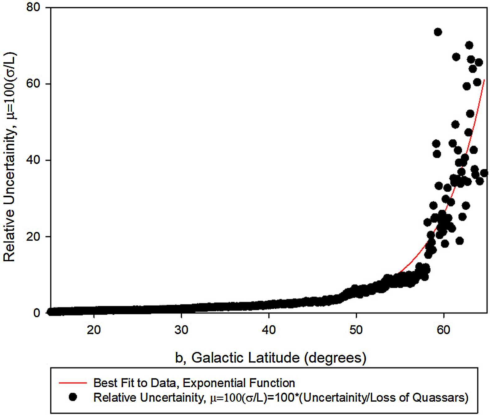
    </mixed-citation>
   </ref>
  </ref-list>
 </back>
</article>