Machine learning algorithms (MLs) can potentially improve disease diagnostics, leading to early detection and treatment of these diseases. As a malignant t
umor whose primary focus is located in the bronchial mucosal epithelium, lung cancer has the highest mortality and morbidity among cancer types, threatening health and life of patients suffering from the disease. Machine learning algorithms such as Random Forest (RF), Support Vector Machine (SVM), K-Nearest Neighbor (KNN) and Na
ïve Bayes
(NB) have been used for lung cancer prediction. However they still face challenges such as high dimensionality of the feature space, over-fitting, high computational complexity, noise and missing data, low accuracies, low precision and high error rates. Ensemble learning, which combines classifiers, may be helpful to boost prediction on new data. However, current ensemble ML techniques rarely consider comprehensive evaluation metrics to evaluate the performance of individual classifiers. The main purpose of this study was to develop an ensemble classifier that improves lung cancer prediction. An ensemble machine learning algorithm is developed based on RF, SVM, NB, and KNN. Feature selection is done based on Principal Component Analysis (PCA) and Analysis of Variance (ANOVA). This algorithm is then executed on lung cancer data and evaluated using execution time, true positives (TP), true negatives (TN), false positives (FP), false negatives (FN), false positive rate (FPR), recall (R), precision (P) and F-measure (FM). Experimental results show that the proposed ensemble classifier has the best classification of 0.9825% with the lowest error rate of 0.0193. This is followed by SVM in which the probability of having the best classification is 0.9652% at an error rate of 0.0206. On the other hand, NB had the worst performance of 0.8475% classification at 0.0738 error rate.
Accuracy False Positive Rate Naïve Bayes Random Forest Lung Cancer Prediction Principal Component Analysis Support Vector Machine K-Nearest Neighbor1. Introduction
The process of automated prediction of disease is key for better treatment and lifesaving. As such, many machine learning (ML) based methods have been developed for various diseases. The growing utilization of machine learning algorithms is attributed to the substantial surge in digital storage of health records, where ML algorithms help in uncovering the patterns existing in these health records. By doing so, interesting insights are gained that assist in the diagnosis of various ailments. Authors in [1] explain that data mining models such as artificial neural networks (ANNs), decision tree (DT) analysis, support vector machines (SVMs), Naïve Bayes (NB), and K-Nearest neighbor (KNN) have been deployed for medical diagnosis. As explained in [2] , the development of newer technologies such as analytics, artificial intelligence, and machine learning has influenced a number of sectors including health care. Here, these schemes are deployed for improving patient wellness, clinical decision support, and better care coordination. Authors in [3] note that there is a growing literature on the deployment of machine learning techniques for the development of psychopathology risk algorithms that inform preventive interventions. For instance, supervised machine learning methods can serve as an alternative to conventional techniques for internalizing disorder (ID). Here, these ML algorithms are critical for the optimization of early detection. World Health Organization (WHO) reports indicate that many cancer cases are diagnosed too late [4] . However, if an accurate diagnosis could be done early, more than 30% of these patients can survive the disease. This calls for the design of effective techniques for early detection of diseases to improve societal healthcare. The complex nature of the actual medical dataset needs careful management due to the serious consequences of prediction errors [5] .
Machine learning (ML) techniques can effectively extract useful knowledge from large, complex, heterogeneous, and hierarchical time series clinical data [6] . As such, many machine learning algorithms have been proposed for deployment in medical diagnosis. As explained in [7] , data mining and machine learning techniques present new and powerful solutions for discovering hidden relationships in complex datasets. In most cases, raw datasets available from different medical science sources have useful information which traditional data classification approaches cannot unravel. In addition, although these manual classification schemes may unravel some latent information, they require longer durations and are prone to human mistakes. Consequently, the provision of reliable and trustworthy predictive models with the highest precision and accuracy is the main goal of data mining and machine learning approaches [7] . It is also important for the predictive models to have negligible error rates for effective diagnosis and treatment. Although machine learning-based techniques have been successful in many areas of medical science, there is a need to optimize and improve these methods [8] . Several techniques are available for lung cancer diagnosis like NB, SVM, and KNN, but those techniques are faced with issues of high-dimensional datasets due to their inability to employ diverse sources of data for prediction, more expensive because of the high computational costs incurred, time consuming and have less capability for detecting lung cancer [9] . As authors in [10] , pointed out, the usage of conventional feature selection techniques has failed to enhance the performance of cancer diagnosis. Authors in [9] , further explain that due to the sensitivity of cancer data, most of the current machine learning algorithms exhibit very low accuracy in their predictions and face high error rates.
Feature selection is a process that involves removing non-relevant and repeated features from a data set to improve the performance of machine learning techniques and their applications. Feature selection has been used to handle the curse of dimensionality in which it has enhanced the performance of data mining and machine learning techniques [11] .
The effectiveness of ML approaches in prediction and classification has endeared them for application in the medical domain. However, the analysis of data from large datasets still remains a challenge such as high computational complexity, high error rates, and missing data values. Moreover, the current machine learning classifiers for cancer prediction are based on gene-level expression data, but there are very few research works on constructing classifiers from transcript-based data. In addition, ML techniques such as RF, SVM, KNN, NB, and genetic algorithms for lung cancer prediction still face challenges such as class imbalance of the training dataset, high dimensionality of feature space, over-fitting, high computational complexity, noise and missing data, low accuracy, low precision and high error rates [12] .
High dimensionality in data sets is one of the challenges that have been experienced in classification, data mining, and sentiment analysis. It results from collecting information with many features or variables that has not been proved to be either needed or significant for the task. These many features have a great impact on the complexity and performance of algorithms that are used for classification. This challenge can be handled through the process of selecting features [13] . This research aims at handling the problem of dimensionality reduction, improve classification accuracy, and minimize false positive rates. This is achieved by using an ensemble classifier consisting of SVM, RF, NB, and KNN. The deployment of PCA is aimed to reduce the feature space for enhanced classification performance. Similarly, ANOVA is deployed to select a subset of the feature space for the 10-fold cross-validation.
Ensemble learning is one such improvement that has enhanced machine learning tasks. Here, a classifier consists of a set of individual classifiers coupled with a mechanism, such as majority voting that combines the predictions of the individual classifiers. Authors in [14] discuss that ensemble classifiers exhibit better performance compared to conventional classifiers. This superiority results from the utilization of a group of decision making systems that apply various strategies to combine classifiers to boost prediction on new data. Authors in [15] concur that ensemble learning can yield more accurate classification results than a single classifier due to the incorporation of benefits from both the performance of different classifiers and the diversity of errors.
This paper proposes an ensemble classifier for selecting features and classifying data that will address the problem of dimensionality reduction, reduce prediction error rates, and provide better performance of classification in terms of their accuracy, precision, recall, false positive rate (FPR) and F-measure using the selected features. Feature selection is done based on Principal Component Analysis (PCA) and Analysis of Variance (ANOVA). An ensemble of classifiers is a set of classifiers whose individual decisions are combined in some way, typically by weighted or unweighted voting to classify new examples. It ultimately aims at selecting the best set of features from the original data that will give a good classification. The classifier is applied to classify lung cancer data set using the SVM, RF, NB, and KNN. The resulting accuracies of the classifiers are investigated without PCA and with PCA deployment, before ANOVA and after ANOVA applications. The proposed classifier has the best classification of 0.9825% with the lowest error rate of 0.0193. This is followed by SVM in which the probability of having the best classification is 0.9625% at an error rate of 0.0206. The contributions of this paper include the following:
i) An ensemble classifier is proposed for leveraging on RF, KNN, NB, and SVM to boost lung cancer detection metrics.
ii) Analysis of variance (ANOVA) is deployed to select a subset of the feature space for the 10-fold cross validation, which shows that the proposed classifier has the highest performance scale.
iii) Principal component analysis (PCA) is deployed to reduce the feature space for enhanced classification performance.
iv) Extensive performance evaluations are executed, which demonstrate that the proposed classifier incurs the lowest false positive rates and the highest classification accuracy compared with other classifiers.
2. Related Work
The field of disease diagnostics has attracted a lot of research efforts from both the industry and academia. This can be attributed to the ease with which diseases such as cancer, diabetes, cardiovascular diseases (CVDs), and Rheumatoid arthritis (RA) can be treated if they are detected early. According to [1] , there is a need to identify the causes of such diseases and be able to diagnosis them early enough. Artificial intelligence-based algorithms have been deployed for this early diagnosis for a number of diseases. For instance, the authors in [16] have applied KNN, ANN, radial basis function (RBF), neural network (RBFNN), and SVM techniques for breast cancer (BC) data classification. In addition, Genetic Algorithm (GA) and Random Forest (RF) algorithms have been deployed for BC detection in [17] . A data mining method for accurate cancer prediction has been developed in [18] , by combining SVMs and ANNs for cancer data analysis. The results showed that this approach improved the performance of the conventional machine learning algorithms, attaining an accuracy of 100%. A probabilistic neural network (PNN), convolutional neural network (CNN), multilayer perceptron neural network (MLPNN), recurrent neural network (RNN) and SVM have been utilized in [19] for cancer prediction. The results showed SVM achieved the best prediction accuracy of 99.54%. On the other hand, the authors in [20] employed a well-known machine learning algorithm (kNN) to examine its execution on the Wisconsin diagnostic breast cancer dataset. The dataset involved 569 instances with 32 attributes and 2 classes. They used two essential dimensionality reduction strategies principal component analysis (PCA) and linear discriminant analysis (LDA) and showed that kNN with LDA technique worked better than kNN and kNN with PCA with the accuracies 97.06%, 95.29%, and 95.88% [21] . Separately, NB techniques in combination with a weighting approach has been deployed in [22] , yielding a BC prediction accuracy of 98.54%.
In [23] , a machine learning method was applied to investigate information regarding lung malignancy, to assess the prescient intensity of these systems. To this aim, a supervised classifier, the k-Nearest-Neighbors (k-NN) algorithm, was first developed using the available datasets to predict lung cancer in its early stages. As the feature selection algorithm can affect the performance of the kNN model, kNN was hybridized with a feature selection genetic algorithm (GA) to classify the risks of lung cancer patients in three levels of low, medium and high. The objective of using GA was to determine the best combination of the features that minimize the overall miscalculation of the kNN method. Moreover, the best value for the number of neighbors in the kNN algorithm was determined using an algorithm coded in Python. This enabled the model to achieve better accuracy in the prediction and prognosis stages. Besides, the value of the parameter k in the kNN algorithm was determined experimentally using an iterative approach. Finally, the performance of the proposed algorithm was assessed when it applies to a lung cancer database. It was shown that when the kNN method is hybridized with a feature selection algorithm, the classification accuracy increases significantly. On comparing performance of the models in terms of their accuracies, the decision trees was at 95.40%, k-NN when k = 1096.40%, k-NN when k = 699.80% and GA + kNN produced 100%.
Supervised learning classification techniques such as linear regression, decision trees, GBM, SVM, and custom ensemble on SEER database was applied in [24] to order lung cancer patients regarding survival. The outcomes demonstrated that among the five individual models used, the most precise was GBM with a root mean square error (RMSE) value of 15.32. In [25] , they employed a combined geneticfuzzy algorithm to diagnose lung cancer. He applied the algorithm to 32 patients with 56 attributes without any reduction in dimensions and attained 97.5% accuracy with a 93% confidence. In their work, [26] developed a hybrid algorithm involving an optimal deep neural network (ODNN) and linear discriminate analysis (LDA) to classify lung nodules as either malignant or benign. In their work, the ODNN was first used to extract important features from computed tomography (CT) lung images. Then, LDA was applied to reduce the dimensionality of the features. Finally, a modified gravitational search algorithm was utilized to optimize the ODNN. The sensitivity, specificity, and accuracy of their algorithm 96.2%, 94.2%, and 94.56%, respectively.
A comparative study was carried out in [27] based on lung cancer detection using machine learning algorithms using lung cancer dataset from UCI Machine Learning Repository and Data World. Classifiers used were included; logistic regression, decision trees, naïve bayes, and SVM. The predictive performances of classifiers were compared quantitatively. The results produced an accuracy of 66.7%, 90%, 87.87%, and 99.2%, respectively. In [28] , they used SVM, NBs, and C4.5 techniques on the North Central Cancer Treatment Group (NCCTG) lung cancer data set to help specialists for better conclusions for cancer survivability rate. In their work [29] , the primary goal was to build a large and reliable lung cancer cohort that could be used for studying lung cancer progression with a set of generalizable approaches. To this end, they combined structured data and unstructured data to identify patients with lung cancer and extract clinical variables. Among the 76,643 patients with at least 1 lung cancer diagnostic code, 42,069 patients were identified as having lung cancer with the classification algorithm. The lung cancer classification model attained an AUC (Area Under the Curve) ROC (Receiver Operating Characteristics) curve (AUROC) of 0.927. By setting a threshold value to achieve a specificity of 90.0%, they achieved a sensitivity of 75.2%, a Positive Prediction Value (PPV) of 94.4%, and an F-score of 0.837.
In their work [30] , developed a weakly supervised learning model using CNN based on EfficientNet-B3 architecture to predict lung carcinoma using a training dataset of 3554 Whole Slide Images (WSIs). Results obtained differentiated between lung carcinoma and non-neoplastic with high Receiver Operating Curve (ROC), Area Under Curves (AUCs) on four tests showed a performance of 0.975 0.974, 0.988 and 0.981 respectively.
On their part [31] , they developed a machine learning classifier to classify available lung cancer data in UCI machine learning repository. The KNN, Naive Bayes (NB) and Radial Basis Function (RBF) network algorithms were used were used to classify data as either cancerous or non-cancerous. The comparison of results revealed that the proposed RBF classifier had resulted with a great accuracy of 81.25% and was thus considered as an effective classifier technique for Lung cancer data prediction.
In another study [32] , developed a computer aided diagnosis (CAD) system supported by artificial intelligence (AI) learning models for effective disease diagnosis. The DT, Support Vector Machine (SVM), Linear Discriminant Analysis (LDA) and Multi-perceptron Neural Networks (MLP-NN) were employed to train and validate the optimal features reduced by the proposed system. By using the 10-fold cross validation, the performance of the model was evaluated using accuracy, f1 score, precision and recall. The study outcome attained 99.62%, 96.88% and 98.21% accuracy on breast, cervical and lung cancer respectively.
In ensemble learning theory, weak learners or base models are called to be used as building blocks for designing more complex models by combining several of them. Most of the time, these basic models perform not so well by themselves either because they have a high bias, i.e. low degrees of freedom models, or because they have too much variance to be robust high-degree-of freedom models. Then, the idea of ensemble methods is to try reducing the bias or variance of such weak learners by combining several of them together to create a strong learner ensemble model that achieves better performance. Table 1 below shows the challenges of conventional machine learning algorithms for lung cancer prediction.
3. Strategy of the Research
In this section, the mathematical basis for the deployed machine learning algorithms is provided. This is followed by data set description, data preprocessing, PCA, and experimentation as explained in the subsections that follow.
3.1. Mathematical Modeling of the Deployed Machine Learning Algorithms for Ensemble Classifier
In this subsection, the mathematical formulations for K-nearest neighbor, Naïve Bayes, Random Forest, and support vector machine are presented.
3.1.1. K-Nearest Neighbours (KNN)
Taking α i as an M-dimensional training vector and β i as the consequent class label, then the training set is formualted as in (1):
{ ( α i , β i ) } i − 1 N ∈ G (1)
Suppose that α ′ is a particular query from some test set ( α ′ , β ′ ) . Based on this, the unknown class label β ′ is derived as shown in steps 2 to 5.
Step 1: Calculate Euclidean distance ℤ between α ′ and each training set ( α i , β i ) :
ℤ ( α ′ , α i ) = ‖ α ′ − α i ‖ ℜ 2 (2)
Equation (2) can also be expressed as follows: suppose that ω is the number of training samples, and Ψ is the number of feature vectors. Then for a particular test feature set ( β 1 , β 2 , β 3 , ⋯ , β n ) and training feature set ( α 1 , α 2 , α 3 , ⋯ , α n ) , ℤ j is derived as in (3):
ℤ j = ∑ i = 1 Ψ ( T e s t i − T r a i n j ) (3)
Step 2: Organize the Euclidean distance ℤ s in ascending order
Step 3: Designate some weight γ i to ith nearest neighbour as in (4):
γ i = 1 ℤ ( α ′ , α i ) 2 (4)
Step 4: For equally weighted KNN rules, designate γ i = 1
Challenges of machine learning algorithms for lung cancer prediction
Author and Year
Dataset
Machine Learning Algorithm
Features
Challenges
Alam et al., 2018; Asada et al., 2020; Radhika et al., 2019
UCI Machine Learning Repository and Data World (Lung cancer dataset)
Support Vector Machine (SVM)
- It is efficient in high dimensional spaces - There is less probability of over-fitting - It can manage linear and nonlinear data - Training time is long when using large data sets It may be difficult to interpret and understand because of problems caused by personal factors and the weights of variables. - The weights of the variables are not constant, thus the contribution of each variable to the output is variant
- The performance - declines while the target classes are overlapping - It is not suitable for vast datasets. - High computational complexity - Prone to over-fitting - With a large dataset, performance goes down - Do not work well when a dataset is noisy
Bharati et al., 2019
Lung cancer dataset
Random Forest
- It has the capability for solving regression and classification issues - It has the capacity to handle the missing values automatically - They do not over-fit - Solve over-fitting a problem in the decision tree
- They are very complex and take more time to build a DT - It is highly expensive because training more deep trees requires more storage space - Computationally expensive training and inference - Missing data imputation - Hard to build accurate and computationally efficient classifiers for medical applications
Günaydin, et al., 2019; Radhika et al., 2019; Pradeep & Naveen., 2018
Lung Cancer dataset
Naïve Bayes (NB)
- Easy to understand and efficient training algorithm - Order of training instances has no effect on training - Useful across multiple domains - Handles discrete and continuous data - Can be used for both binary and multi-classification - Not sensitive to irrelevant features
- Feature interactions cannot be integrated - Assumes attributes are statistically independent - Assumes normal distribution of numerical attributes - Redundant attributes mislead classification - attributes and class frequencies affect accuracy - Computationally intensive especially, for models including many variables
NegarMaleki et al. (2020); Chinmayi, Aarsha and Sagi., (2020); Kavit et al., (2018)
Lung Cancer dataset
K-Nearest Neighbour (KNN)
- Training is very quick. - It is easy and simple to implement - It is easy and simple to implement - Tolerant of noisy instances or instances with missing attribute value - works on concept that samples in nearby space are likely to fit in the alike class
- It requires more memory space - The testing procedure is quite slow and the noise is very sensitive - Noisy and irrelevant features resulted in degradation of accuracy - Too computationally complex as number of attributes increases - A lazy algorithm that needs more time to run - High dimensionality of the feature space and imbalance in the size of the samples of the target classes - Inaccurate or mislabeled training data which presents some noise in ML training data
Step 5: Suppose F ( . ) is the Dirac-delta function, η is the class label, and β ′ is the class label for ith nearest neighbour among its K-nearest neighbours. Then depending on the majority vote of its nearest neighbours, the class label for α ′ is assigned as in (5):
β ′ = arg max η ∑ ( α i , β i ) ∈ G ′ γ i F ( η = β ′ ) (5)
Here, F ( . ) assumes the value of unity (1) when its argument is true and zero otherwise.
3.1.2. Support Vector Machine (SVM)
This classifier takes in an input feature vector and establishes the class to which this vecor belongs to. Suppose that α i , i = 1 , 2 , 3 , ⋯ , N are the feature vectors for training set Ť. Here, Ť may belong to either Ÿ1 or Ÿ2. Based on this training data, the hyperplane is mathematicaly represented as in (6):
ℍ ( α ) = γ d α i + L = 0 (6)
where γ = [ γ 1 , γ 2 , ⋯ , γ q ] represents the weight vector and L is the bias. Here, the binary classification degenerates into the solution of the decision function in (7):
℘ ( α ) = sign ( γ d α i + L ) (7)
Due to the possibility of many hyperplanes that separate the feature vectors, the role of SVM is to find the one with the largest margin. For non-linearly separable feature vectors, the input space is mapped into high-dimensional feature space using kernel function that transform it into linear separable. In essense, kernel functions serve to transform feature vectors from finite to infinite dimensional space. As such, the performance of SVM is influenced immensely by the underlying kernel function. The five most prominent kernel functions include linear, Mahalanobis, radial basis function(RBF), polynomial, and sigmoid (also known as hyperbolic tangent or multilayer perception kernel) whose mathematical formulations are derived in (8) to (12).
In these formulations, M ( > 0 ) is the scaling factor, D is the dimension of the data set, V is the covariance matrix, and denotes the polynomial kernel degree, which is adjustable just like the parameters and based on the underlying data.
K ( α i , α j ) = 1 + α i d α j , (linear) (8)
, (Polynomial) (9)
, (RBF or Gaussian) (10)
K ( α i , α j ) = − M D ( α i − α j ) d V − 1 ( α i − α j ) (Mahalanobis) (12)
In Equation (10), M serves to control the Mahalanobis distance.
Consdering a set of q data samples that belong to two classes ( α 1 , β 1 ) , ( α 2 , β 2 ) , ⋯ , ( α q , β q ) that are mapped to a higher dimensional space, where β i ∈ { − 1 , 1 } . For the correct classification process, the separating hyperplane should be optimized. Taking γ as some weight vector and L as the bias weight, the optimization problem in SVM degenerates to the determination of the hyperplane that segrates the positive and negative classes given in (14) and (15):
ℍ ( α ) = γ α i + L = 0 (13)
γ α i + L ≥ 1 , for β i = 1 (14)
γ α i + L ≤ − 1 , for β i = − 1 (15)
To accomplish this, the margin between the two classes is maximized by determining γ and L that maximizes (16):
1 2 ‖ γ ‖ 2 (16)
In essence, an optimal hyperplane denotes an error-free plane with the largest possible separation margin. Ideally, this is the hyperplane that minimizes the cost function in (17):
ℂ ( γ ) = 1 2 γ d ⋅ γ (17)
The optimization in (17) is subject to some constants in (18):
β i ( γ d ⋅ α i + L ) ≥ 1 , i = 1 : q (18)
Due to the convex nature of ℂ ( γ ) , Lagrange multipliers ( l 1 , l 2 , ⋯ , l q ) are employed to reduce this constrained optimization problem. This is achieved through the process of weighing each data point based on its criticality in the determination of the segregating information of the two classes. Mathematically, this is derived as in (19):
max L ( γ , L , l ) = ∑ i = 1 q l i − 1 2 ∑ i = 1 q ∑ j = 1 q l i l j β i β j ( α i . α j ) (19)
The optimization in (19) is subject to the conditions in (20):
l i ≥ 0 & ∑ i = 1 q l i β i = 0 (20)
Incorporating Lagrange multipliers to the decision function in (7) results in (21):
℘ ( α ) = sign ( ∑ i = 1 q l i β i ( α i . α ) + L ) (21)
Taking ℂ ( α ) as the transformation function that maps lower dimension feature vectors to the higher dimensional feature space, then the kernel function in (22) is deployed for these transformations:
K ( α , β ) = ℂ ( α ) ℂ ( β ) (22)
Based on (22), the decision function is modified as in (23):
℘ ( α ) = sign ( ∑ i = 1 q l i β i K ( α i , α ) + L ) (23)
3.1.3. Random Forest (RF)
This classifier comprises of a classification tree T ( J , K i ) , i = 1 , 2 , ⋯ , q . Here, K i represents a vector that is identically and indepently disributed (IID) to each tree vote at its input J. In short, a random forest combines several decision trees to minimize overfitting. Suppose that T 1 ( S ) , T 2 ( S ) , ⋯ , T q ( S ) is an ensemble classifier with arbitrary training data got from vector S and Q (the prediction class), f is the indicator function, A ⌣ is the mean, the margin function is formulated as in (24):
m g ( S , Q ) = A ⌣ f ( T 1 ( S ) = Q ) − max R ≠ Q f ( T 1 ( S ) = R ) (24)
In (24), T i ( S ) = Q denote classification result while T i ( S ) = R is classification result with R. In RF, the margin is utilized to establish the mean value of votes S and Q, such that the greater the margin, the more accurate is the classification. Here, the generalization error G ^ is derived as in (25):
G ^ = W S , Q ( m g ( S , Q ) < 0 ) (25)
In (25), WS,Q signifies thatthe probability is more than S, Q dimension. Considering training sample Ţ p = { ( α 1 , β 1 ) , ⋯ , ( α p , β p ) } of IID [ 0 , 1 ] l . Using Ţp, the objective is to estimate the regression function R F ( α ) = E [ β [ α = g ] ] for some fixed g ∈ [ 0 , 1 ] l . Generally, RF classifier consists of a set of stochastic regression tree { R T ( g , h q , Ţ p ) , q ≥ 1 } . Here, h 1 , h 2 , ⋯ Denotethe IID outputs of a randomization construct h. By combining these random trees (RTs), an amalgamated regression estimate is obtained as in (26):
R ¯ T ( α , Ţ p ) = E h [ R T ( g , h , Ţ p ) ] (26)
In (26), E h is conditionally associated with random constructs on g and Ţp. Here, the dependency of sample estimates is denoted as R ¯ T ( g ) and h is utilized to establish how successive divisions are executed when building individual trees.
3.1.4. Naïve Bayes
In this algorithm, the probability that an attribute g takes on a particular G when the class is Ƈ is modeled using a real number between 0 and 1. On the other hand, continuous attributes are modeled using continuous probability distribution over a range of attribute’s values. Suppose that RV is a random variable representing an instance class, and RA is a random variable vector representing the observed attribute values. Denoting rv as a specific class label and ra as the specific observed attribute value, then if Ʀ is a test case, that is to be classified, the probability of each class given the vector of observed values for the predicitive features is obtained using Bayes’ theorem in (27):
p ( R V = r v | R A = r a ) = p ( R V = r v ) p ( R A = r a | R V = r v ) p ( R A = r a ) (27)
Since an event consists of a juxtaposition of feature value and assignments, then using the feature conditional independence postulation, Equation (27) is written as in (28):
p ( R A = r a | R V = r v ) = ∏ i p ( R A i = r a i | R V = r v ) (28)
Suppose that Ƥ is the training set and Ū is the related class label. Here, each tuple is denoted by Ȅ features, implying that each tuple consists of Ȅ values. If there are k class labels U ¯ 1 , U ¯ 2 , ⋯ , U ¯ k for any new tuple Z, the classifier predicts that Z is a member of the class with highest probability state on Z, suppose now that this classifier is presented with a new test set Z that needs to be classified as either benign or malignant. Here, Z can be classified into its respective class U ¯ i or U ¯ j provided it satisfies the state in (29):
P ( Ū i Z ) > P ( Ū j Z ) for 1 ≤ j ≤ k (29)
In this case, U ¯ i becomes the maximum posterior hypothesis since its ( Ū i Z ) is being maximized. Based on Bayes’s theorem:
P ( U ¯ i | Z ) = P ( Z | U ¯ i ) P ( U ¯ i ) P ( Z ) (30)
Since P(Z) is unvarying for the classes, only the value for P ( Z | U ¯ i ) P ( U ¯ i ) need to be increased. In this case, the formualions reduce to:
P ( U ¯ i Z ) = P ( Z U ¯ i ) ∗ P ( U ¯ i ) (31)
During the prediction of Z’s class label P ( Z U ¯ i ) ∗ P ( U ¯ i ) is evaluated for each class U ¯ i . In essence, the predictor class label U ¯ i for which P ( Z U ¯ i ) ∗ P ( U ¯ i ) is maximum.
On the condition that apriori probability for class P ( U ¯ j ) is unknown, the assumption made is that the classes are all equally likely and P ( Z | U ¯ j ) needs to be maximized.
During the class label or class value Z classification P ( Z | U ¯ i ) P ( U ¯ i ) is evaluated for both benign and malignant instances in U ¯ i . In this case, NB classifies Z to a class U ¯ i on the condition that it is the class that maximizes P ( Z | U ¯ i ) P ( U ¯ i ) .
3.2. Data Set Description
In this paper, the data set from the ELVIRA Biomedical Data Set Repository [33] , which consists of both normal genetic sequences as well as lung tumor sequences, was used. The data contains 203 specimens, consisting of 139 samples of lung adenocarcinomas, 21 samples of squamous cell lung carcinomas, 20 samples of pulmonary carcinoids, 6 samples of small-cell lung carcinomas, and 17 normal lung samples. Here, each sample is described by 12600 genes. This data set is partitioned into an 80% training data set and 20% testing data set. The dataset is accessed using this link: http://leo.ugr.es/elvira/DBCRepository/.
3.3. Data Pre-Processing
The dataset accessed in this paper contains missing values and noisy information. Therefore, before the classification process, the data was cleansed and relevant analysis excuted to eliminate redundant attributes for further analysis. Thereafter, a data transformation is executed to map the attribute values to a small-scale range of 1 or 0, before the application of PCA for dimensionality reduction. The Bin smoothing using the minimax approach was adopted for cleaning and tarnsformation. Principal Component Analysis (PCA) and Analysis of Variance (ANOVA) were utilized to get rid of datasets with huge dimensions that could lead to over-fitting.
Binning is a technique for smoothing noisy values by consulting their neighbourhood. This requires that the data be sorted in some order before it is partitioned into a specific number of bins. Thereafter, smoothing is accomplished by bin means, median or bin boundary. Taking L as the lowest value of a certain feature, H as the highest value of a feature, then the width of intervals, Ɯ is given by (32):
Ɯ = H − L hυ (32)
where ƕ is the number of partitions.
3.4. Principal Component Analysis
Based on the deployed data, its input attributes are considerable and this may impede the classification speed and accuracy. As such, the principal component analysis (PCA) is utilized for feature selection as one way of dimensionality reduction in the input features. The selection of PCA was informed by the fact that it is a simple and yet widely deployed dimensionality reduction technique for two-class classification problems. In essence, PCA serves to establish the peak disparity in the underlying data set. In so doing, many features in the dataset are reduced to less but crucial features. By applying it to both training and testing samples, patterns in the input dataset are detected based on the resemblance and variance among the present attributes. Suppose that M is the dimension of the data set that has q samples { N i } i = 1 q , in which N i ∈ R M . Here, PCA attempts to determine the principle orthogonal directions in which this data set has the highest variances. Provided that the majority of these variances occur in one or numerous main directions, these directions form the principal component directions of the data set. These directions are a better representation of the data set with less dimensions. Taking V ˜ as the mean vector of the data samples, the covariance matrix Ω of the sample set is computed as in (32):
Ω = E [ ( N i − V ˜ ) ( N i − V ˜ ) T ] (32)
Using the eigenvectors of Ω as the basis to span a new coordinate system, the orthogonal coordinate system can be obtained that can eliminate the correlations between diverse components of the samples in their initial space. Essentially, the levels of Ω’s eigenvalues depict the variance of the samples along the coordinates of the consequent eigenvalues. Suppose that we have an H × G matrix denoted by ℚ , in which each row refers to one of H trials while each column denotes one of G features. We also let B ℚ represent the average of the input, in which case the Eigen values (λi) and Eigen vectors (μi) of the input correlation matrix are derived as in (33):
Σ = E ¯ T E ¯ (33)
In which E ¯ = ℚ − B ℚ
Taking Q ¯ as the right singular vector, the principal components are expressed as in (34):
P = E ¯ ⋅ Q ¯ T (34)
Suppose that ( λ 1 , λ 2 , ⋯ , λ q ) are the eigenvalues of matrix Ω, they can be ordered based on their size as: λ 1 ≥ λ 2 ≥ ⋯ ≥ λ q . Denoting the corresponding eigenvectors as ( μ 1 , μ 2 , ⋯ , μ q ) , if the first λs are very large compared with the rest, only μs corresponding to these λs are utilized to represent the data set without significant loss of the information. The deployed μs are the principal component axes of the data set, while the spanned subspace by these μs forms the principal component space (PCS). When the first n μs are deployed to build the PCS, the resulting representation error of truncation error e is derived as in (35):
e = ∑ i = n + 1 M λ i ∑ i = 1 M λ i (35)
This PCA depiction has the minimum error among the feasible orthogonal n-dimensional representations of the sample set. The follwing feature determination rules were applied:
Feature standardization: after feeding the ELVIRA datasent to PCA, each feature is transfomed in such a way that its mean and variance are 0 and 1 respectively. This procedure facilitates selection of the best principal components.
Computation of the covariance matrix: this involves the derivation of the pairwise correlation between each of the features which is the covariance matrix of the feature space.
Calculation of the eigenvectors and equivalent eigenvalues for the covariance matrix
Arranging the eigenvectors in descending order: here the computed eigenvectors are arranged in descending order based on eigenvalues. In essence, the eigenvectors with the highest eigenvalue becomes the first principal component.
Selection of the number of principal components: in this, the top N eigenvectors are selected based on their corresponding eigenvalue. In this, the choses eigenvectors represent the N principal components.
3.5. Results and Discussion
Upon data preprocessing, four machine learning algorithms which include KNN, SVM, RF, and NB are applied to the obtained data.
Data preprocessing was carried out to remove irrelevant and inconsistent data to increase prediction and reliability of the output. Bin smoothing was used for cleaning and data transformation. Feature extraction was done using Principal component analysis. The analysis of variance (ANOVA) was used to establish the statistical significance of the differences between the feature set means. Thereafter an ensemble classifier was developed based on KNN, SVM, RF and NB.
3.5.1. Proposed Ensemble Classifier
In this paper, an ensemble classifier is developed consisting of KNN, SVM, RF, and NB. This choice is informed by the fact that these four machine learning algorithms are the most prevalent in lung cancer diagnosis. Past research has shown that ensemble classifiers outperform their single classifier equivalents. Therefore, a blending approach is employed in this paper where the same ELVIRA dataset is fed to each of the individual classifiers. Thereafter, each of these models is trained and tested. As shown in Figure 1, the output of this classifier is obtained via majority voting.
As shown in Figure 1, the first step during ensemble classification is the feeding of the ELVIRA dataset to PCA algorithm which executes the dimensionality reduction in this dataset. The algorithm for PCA is elaborated in Figure 2. After feature selection, the ELVIRA dataset is split into two sets; 80% for training and the other 20% for testing the classifiers. These two sets of data are then fed to the individual classifiers after which individual predictions are performed. Suppose that KNN, SVM, RF and NB votes 1, 1, 1 and 0 respectively. The implication is that KNN, SVM, and RF prediction is lung cancer presence, while NB has predicted lung absence. Using majority voting, the final prediction is lung cancer presence since we have 3 classifiers voting for 1 while only one classifier has voted for 0.
To accomplish this, Waikato with Environment for Knowledge Analysis (WEKA) software was utilized. This choice was informed by its ability to implement and facilitate the analysis of numerous classification, regression, and data mining algorithms. Figure 3 gives the general data flow diagram for the machine leaning algorithm (MLA) classification process. As shown in Figure 1, the lung cancer classification comprised of a number of steps, starting with the feeding of the data set to the MLA upon which data processing was executed. This is followed by training and testing the classifiers. The 10-fold cross validation test is utilized to evaluate the developed predictive models. This technique simply partitions the data set into training and test samples. Here, the training data sample is used to build the model while the test sample evaluates the constructed model. Here, the classification involves the correct placement of an instance into either the B or M class.
The last set of experimentations involved the appraisal of the performance of individual classifiers using the performance metrics in Table 2 below. Here, TP is true positive, TN is true negative, FP is false positive, and FN is false negative. Accuracy represented the overall correctness of the model, while precision depicts the ratio of positive cases that were predicted appropriately. On the other hand, the FP-rate is the ratio of negative cases that were incorrectly classified as positive cases. Recall or TP rate represents the ratio of correctly identified positive cases while F-measure is the harmonic mean of precision and recall.
In terms of error performance, Mean Absolute Error (MAE), Kappa, Root Mean Squared Error (RMSE), Relative Absolute Error (RAE), and Root Relative Squared Error (RRSE) are deployed. Table 3 gives the formulations of these errors.
In Table 3, y i is the predicted value, y i j is the predicted value by individual model i for tuple j out of n tuples, T j is the target value for tuple j, x i is the actual value, while n is the number of data points.
The results obtained for the various metrics are presented in Section 4. Thereafter, the interpretation of these findings is provided as discussed below.
The developed classifiers are evaluated in terms of their build time, true positives (TP), true negatives (TN), false positives (FP), false negatives (FN), FP rate (FPR), recall (R), precision (P) and F-measure (FM). Next, analysis of variance (ANOVA) is deployed to establish the statistical significance of the differences between the feature set means.
Performance metrics
Metric
Formulation
Accuracy
T P + T N T P + T N + F P + F N
FP-rate
F P F P + T N
Precision
T P T P + F P
Recall / TP-rate
T P T P + F N
F-measure
2 ∗ Pr e c i s i o n ∗ Re c a l l Pr e c i s i o n + Re c a l l
Error analysis
Error
Formulation
MAE
∑ i = 1 n | y i − x i | n
Kappa
2 ∗ ( ( T P ∗ T N ) − ( F N ∗ F P ) ) ( T P + F P ) ∗ ( F P + T N ) + ( T P + F N ) ∗ ( F N + T N )
RMSE
1 n ∑ i = 1 n ( x i − y i ) 2
RAE
[ ∑ i = 1 n ( y i − x i ) 2 ] 1 / 2 [ ∑ i = 1 n x i 2 ] 1 / 2
RRSE
∑ j = 1 n ( y i j − T j ) 2 ∑ j = 1 n ( T j − T _ ) 2 , where T _ = 1 n ∑ j = 1 n T j
3.5.2. ANOVA Algorithm
In this paper, Analysis Of Variance (ANOVA) is deployed to establish the statistical significance of the differences between the feature set means. This is a five-step process as shown in Figure 3. It begins with the formulation of the hypothesis, calculation of the sum of squares, determination of the degree of freedom, computation of F-value, and then finally the acceptance or rejection of the null hypothesis. In this paper, the null hypothesis is that all features in the feature space have the equal variance.
It follows that the alternative hypothesis is that at least one of the features in the ELVIRA dataset has different variance. On the other hand, the sum of squares is computed as ∑ i = 0 ( A i − A ¯ ) 2 . Here, Ai is the ith feature in the feature space, A ¯ is the mean of all features in the feature space and ( A i − A ¯ ) is the deviation of the feature from this mean. The next step is the derivation of the degree of freedom as (N-1), where N denotes the feature space. This is followed
by the computation of F-value as ( C 1 2 N 1 − 1 / C 2 2 N 2 − 1 ) . Here, C 1 and C 2 are Chi distributions while N 1 and N 2 are their respective degrees of freedom. Based on the 95% confidence level and the computed degrees of freedom, the calculated F-value is deployed to accept or reject the null hypothesis.
4. Results and Discussion
In this section, the performance of the ensemble classifier is reported for before and after ANOVA application. After ANOVA application, 10-fold cross-validation is employed to evaluate the performance of these classifiers after feature selection optimization. Figure 4 presents the build time for various classifier models. Based on the values in Figure 4, the proposed classifier incurs the highest build time of 0.31 seconds among other models.
This can be explained by the amalgamated build time for the models that make up this ensemble classifier. However, among the individual classifiers, RF
takes the longest duration of 0.29 seconds to build the model, while KNN took the shortest duration of 0.01 seconds. The explanation for this is that KNN is a lazy learner and hence it does not execute many operations during training. This is unlike other MLAs which need to build models during the training process. Next, the accuracies of the classifiers are investigated without PCA and with PCA deployment. As shown in Figure 5, there is a general increment of accuracy in the models when PCA is applied. It follows from Figure 5 that the accuracies before PCA application for RF, SVM, NB, KNN, and the proposed classifier are 92.2%, 95.5%, 90.1%, 94.7%, 97.5% respectively. However, after PCA application, the accuracies for RF, SVM, NB, KNN, and the proposed classifier are 95.1%, 98.6%, 92.3%, 96.5%, and 99.3% respectively. Considering only the individual classifiers with PCA, SVM, has the highest value of 98.6%, while NB has the lowest value of 92.3%.
This directly follows from SVM’s highest values for TP/TN and lowest value for FP/FN compared to other classifiers. On the other hand, Figure 6 shows the performance of these classifiers in terms of the FPR before and after PCA application.
Based on the graphs in Figure 6, the FPR for RF, SVM, NB, KNN, and the proposed classifier before PCA application are 0.0731, 0.039, 0.12, 0.062, and
0.029 respectively. However, after PCA application, the FPR for RF, SVM, NB, KNN, and the proposed classifier are reduced to 0.067, 0.023, 0.090, 0.042, and 0.012 respectively. It is evident from Fig.6.0 that after PCA, NB classifier has the highest FPR of 0.090. This is followed by RF, KNN, and SVM with FPR values of 0.067, 0.042, and 0.023 respectively. On the other hand, the proposed ensemble classifier has the lowest FPR value of only 0.012. In terms of recall(R), precision(P) and F-measure(FM), Figure 7 presents the values obtained before the ANOVA application.
It is evident from Figure 7 that the proposed classifier has the highest values for recall, precision and F-measure whose values are 0.993, 0.997 and 0.995. On the other hand, the NB classifier has the lowest scores for recall, precision and F-measure whose values are 0.923, 0.921, and 0.922. Table 4 presents the error performance for the various classifiers.
It is clear from Table 4 that among individual classifiers, in SVM, the probability of obtaining the best classification is 0.9652% with the lowest error rate of 0.0206. On the other hand, NB has the worst performance of 0.8475% classification
Error performance
Error
Classifiers
NB
RF
KNN
SVM
Proposed
MAE
0.0738
0.0749
0.0407
0.0206
0.0193
Kappa
0.8475
0.9026
0.9238
0.9652
0.9825
RMSE
0.2637
0.1748
0.1959
0.1462
0.1298
RAE
15.7832
16.1648
8.6572
4.5142
4.7183
RRSE
54.7826
35.7492
40.5630
30.0195
28.2621
with 0.0738 error rate. It is evident that both NB and RF have highest error rates which can be attributed to their high (ICI) values. In overall, the proposed classifier’s probability of obtaining best classification is 0.9825% with an error rate 0.0193. Consequently, it has the best overall error rate performance. Using the analysis of variance (ANOVA), the next task was the establishment of the statistical significance of the differences between the feature means. At the 95% confidence level, 8825 features out of the 12601 features had p-values of less than 0.05. Figure 8 shows the performance of the classifiers after the application of ANOVA.
Comparing the graphs in Figure 8 with ones in Figure 7, it is evident that there is some slight improvements in the values of recall, precision and F-measure across all the classifiers. This is attributed to the feature selection optimization that is accomplished through ANOVA where 3776 features whose p-values are more than 0.05 are eliminated from the training and testing. Next, this sub-set of features were deployed for the 10-fold cross validation of the classifiers. This basically provided the basis for the evaluation of the proposed ensemble classifier. Figure 9 shows the performance scales of these classifiers during the 10-fold cross-validation.
Based on the graphs in Figure 9, NB classifier has the worst performance of 91.6% while the proposed classifier has the best performance of 98.6%. On the
other hand, the performance scales for RF, SVM, and KNN are 95.7%, 97.9%, and 96.1% respectively. In overall, the deployed techniques such as PCA, ANOVA, and majority voting have been demonstrated to boost performance of lung cancer diagnosis. In all the training, testing and validation instances, the proposed ensemble classifier has demonstrated the best performance overall, the NB classifier has shown worst performance in all the performance metrics. On the other hand, the SVM classifier has the second best performance while KNN has the third best performance in all the deployed metrics.
5. Conclusion and Future Work
Lung cancer is one of the most common diseases whose early detection can potentially save lives. However, designing a machine learning model for the detection of this disease presents some challenges due to its heterogeneous nature. In addition, performance evaluation of lung cancer machine learning models has been noted to be cumbersome. In this paper, an ensemble machine learning algorithm is developed based on RF, SVM, NB, and KNN. Here, lung cancer classification starts by feeding of the data set to the machine learning algorithm upon which data processing is executed. This is followed by training and testing the classifiers, after which 10-fold cross-validation test is utilized to evaluate the developed predictive models. Experimental results show that the proposed classifier has the highest classification performance of 0.9825% with the lowest error rate of 0.0193. This is followed by SVM in which the probability of having best classification is 0.9652% with an error rate of 0.0206. On the other hand, NB had the worst performance of 0.8475% classification with 0.0738 error rate. Future work in this research domain will involve building an ensemble classifier encompassing other machine learning algorithms that were not within the scope of the current work. There is also a need to evaluate the developed ensemble classifier in other data sets to offer a more comprehensive overview of its performance.
Funding
This work did not receive any financial support or any grant from any organization whatsoever.
Data Availability Statement
The dataset is accessed using this link: http://leo.ugr.es/elvira/DBCRepository/.
Conflicts of Interest
No conflict of interest, financial or otherwise, is declared by the author.
Cite this paper
Abuya, T.K. (2023) Lung Cancer Prediction from Elvira Biomedical Dataset Using Ensemble Classifier with Principal Component Analysis. Journal of Data Analysis and Information Processing, 11, 175-199. https://doi.org/10.4236/jdaip.2023.112010
ReferencesLiu, N., Li, X., Qi, E., Xu, M., Li, L. and Gao, B. (2020) A Novel Ensemble Learning Paradigm for Medical Diagnosis with Imbalanced Data. IEEE Access, 8, 171263-171280.Yekkala, I., Dixit, S. and Jabbar, M.A. (2017) Prediction of Heart Disease Using Ensemble Learning and Particle Swarm Optimization. Proceedings of the 2017 International Conference on Smart Technologies for Smart Nation (SmartTechCon), Bengaluru, 17-19 August 2017, 691-698. https://doi.org/10.1109/SmartTechCon.2017.8358460Rosellini, A.J., Liu, S., Anderson, G.N., Sbi, S., Tung, E.S. and Knyazhanskaya, E. (2020) Developing Algorithms to Predict Adult Onset Internalizing Disorders: An Ensemble Learning Approach. Journal of Psychiatric Research, 121, 189-196. https://doi.org/10.1016/j.jpsychires.2019.12.006Jiang, J., Li, X., Zhao, C., Guan, Y. and Yu, Q. (2017) Learning and Inference in Knowledge-Based Probabilistic Model for Medical Diagnosis. Knowledge-Based Systems, 138, 58-68. https://doi.org/10.1016/j.knosys.2017.09.030Baccouche, A., Garcia-Zapirain, B., Castillo Olea, C. and Elmaghraby, A. (2020) Ensemble Deep Learning Models for Heart Disease Classification: A Case Study from Mexico. Information, 11, Article 207. https://doi.org/10.3390/info11040207Eshtay, M., Faris, H. and Obeid, N. (2018) Improving Extreme Learning Machine by Competitive Swarm Optimization and Its Application for Medical Diagnosis Problems. Expert Systems with Applications, 104, 134-152. https://doi.org/10.1016/j.eswa.2018.03.024Alkeshuosh, A.H., Moghadam, M.Z., Al Mansoori, I. and Abdar, M. (2017) Using PSO Algorithm for Producing Best Rules in Diagnosis of Heart Disease. Proceeding of 2017 International Conference on Computer and Applications (ICCA), 6-7 September 2017, Doha, 306-311. https://doi.org/10.1109/COMAPP.2017.8079784Sevakula, R.K. and Verma, N.K. (2017) Assessing Generalization Ability of Majority Vote Point Classifiers. IEEE Transactions on Neural Networks and Learning Systems, 28, 2985-2997. https://doi.org/10.1109/TNNLS.2016.2609466Mazlan, A., Sahabudin, N., Remli, M., et al. (2021) A Review on Recent Progress in Machine Learning and Deep Learning Methods for Cancer Classification on Gene Expression Data. Processes, 9, Article 1466. https://doi.org/10.3390/pr9081466Nanglia, P., Kumar, S., Mahajan, A.N., Singh, P. and Rathee, D. (2021) A Hybrid Algorithm for Lung Cancer Classification Using SVM and Neural Networks. ICT Express, 7, 335-341. https://doi.org/10.1016/j.icte.2020.06.007Bolón-Canedo, V., Sánchez-Maroño, N. and Alonso-Betanzos, A. (2015) Recent Advances and Emerging Challenges of Feature Selection in the Context of Big Data. Knowledge-Based Systems, 86, 33-45. https://doi.org/10.1016/j.knosys.2015.05.014Baker, Q., Gharaibeh, M. and Al-Harahsheh, Y. (2021) Predicting Lung Cancer Survival Time Using Deep Learning Techniques. Proceeding of 2021 12th International Conference on Information and Communication Systems (ICICS), Valencia, 24-26 May 2021, 177-181. https://doi.org/10.1109/ICICS52457.2021.9464589Nguyen, T.H., Shirai, K. and Velcin, J. (2015) Sentiment Analysis on Social Media for Stock Movement Prediction. Expert Systems with Applications, 42, 9603-9611. https://doi.org/10.1016/j.eswa.2015.07.052Li, H., Cui, Y., Liu, Y., Li, W., Shi, Y., Fang, C. and Lu, Y. (2018) Ensemble Learning for Overall Power Conversion Efficiency of the All-Organic Dye-Sensitized Solar Cells. IEEE Access, 6, 34118-34126. https://doi.org/10.1109/ACCESS.2018.2850048Zhang, X. and Mahadevan, S. (2019) Ensemble Machine Learning Models for Aviation Incident Risk Prediction. Decision Support Systems, 116, 48-63. https://doi.org/10.1016/j.dss.2018.10.009Mert, A., Kılıç, N., Bilgili, E. and Akan, A. (2015) Breast Cancer Detection with Reduced Feature Set. Computational and Mathematical Methods in Medicine, 2015, Article ID: 265138. https://doi.org/10.1155/2015/265138Aličković, E. and Subasi, A. (2017) Breast Cancer Diagnosis Using GA Feature Selection and Rotation Forest. Neural Computing and Applications, 28, 753-763. https://doi.org/10.1155/2015/265138Abdar, M. and Makarenkov, V. (2019) CWV-BANN-SVM Ensemble Learning Classifier for an Accurate Diagnosis of Breast Cancer. Measurement, 146, 557-570. https://doi.org/10.1016/j.measurement.2019.05.022übeyli, E.D. (2007) Implementing Automated Diagnostic Systems for Breast Cancer Detection. Expert Systems with Applications, 33, 1054-1062. https://doi.org/10.1016/j.eswa.2006.08.005Joshi, A. and Mehta, A. (2018) Analysis of K-Nearest Neighbor Technique for Breast Cancer Disease Classification. International Journal of Recent Scientific Research, 9, 26126-26130.Chhatkuli, R.B., Demachi, K., Miyamoto, N., Uesaka, M. and Haga, A. (2015) Dynamic Image Prediction Using Principal Component and Multi-Channel Singular spectral Analysis: A Feasibility Study. Open Journal of Medical Imaging, 5, 133-142. https://doi.org/10.4236/ojmi.2015.53017Karabatak, M. (2015) A New Classifier for Breast Cancer Detection Based on Naïve Bayesian. Measurement, 72, 32-36. https://doi.org/10.1016/j.measurement.2015.04.028Maleki, N., Zeinali, Y. and Niaki, S.T.A. (2021) A k-NN Method for Lung Cancer Prognosis with the Use of a Genetic Algorithm for Feature Selection. Expert Systems with Applications, 164, Article ID: 113981. https://doi.org/10.1016/j.eswa.2020.113981Lynch, C.M., Abdollahi, B., Fuqua, J.D., de Carlo, A.R., Bartholomai, J.A., Balgemann, R.N. and Frieboes, H.B. (2017) Prediction of Lung Cancer Patient Survival via Supervised Machine Learning Classification Techniques. International Journal of Medical Informatics, 108, 1-8. https://doi.org/10.1016/j.ijmedinf.2017.09.013Alharbi, A. (2018) An Automated Computer System Based on Genetic Algorithm and Fuzzy Systems for Lung Cancer Diagnosis. International Journal of Nonlinear Sciences and Numerical Simulation, 19, 583-594. https://doi.org/10.1515/ijnsns-2017-0048Lakshmanaprabu, S.K., Mohanty, S.N., Shankar, K., Arunkumar, N. and Ramirez, G. (2019) Optimal Deep Learning Model for Classification of Lung Cancer on CT Images. Future Generation Computer Systems, 92, 374-382. https://doi.org/10.1016/j.future.2018.10.009Radhika, P.R., Nair, R.A.S. and Veena, G. (2019) A Comparative Study of Lung Cancer Detection Using Machine Learning Algorithms. Proceedings of 2019 IEEE International Conference on Electrical, Computer and Communication Technologies (ICECCT), Coimbatore, 20-22 February 2019, 1-4. https://doi.org/10.1109/ICECCT.2019.8869001Pradeep, K.R. and Naveen, N.C. (2018) Lung Cancer Survivability Prediction Based on Performance Using Classification Techniques of Support Vector Machines, C4.5 and Naive Bayes Algorithms for Healthcare Analytics. Procedia Computer Science, 132, 412-420. https://doi.org/10.1016/j.procs.2018.05.162Yuan, Q., Cai, T., Hong, C., et al. (2021) Performance of a Machine Learning Algorithm Using Electronic Health Record Data to Identify and Estimate Survival in a Longitudinal Cohort of Patients with Lung Cancer. JAMA Network Open, 4, e2114723. https://doi.org/10.1001/jamanetworkopen.2021.14723Kanavati, F., Toyokawa, G., Momosaki, S., Rambeau, M., Kozuma, Y., Shoji, F., et al. (2020) Weakly-Supervised Learning for Lung Carcinoma Classification Using Deep Learning. Scientific Reports, 10, Article No. 9297. https://doi.org/10.1038/s41598-020-66333-xHsu, C.H., Chen, X., Lin, W., Jiang, C., Zhang, Y., Hao, Z. and Chung, Y.C. (2021) Effective Multiple Cancer Disease Diagnosis Frameworks for Improved Healthcare Using Machine Learning. Measurement, 175, Article ID: 109145. https://doi.org/10.1016/j.measurement.2021.109145Solanki, A., Kumar, S., Rohan, C., Singh, S.P. and Tayal, A. (2021) Prediction of Breast and Lung Cancer, Comparative Review and Analysis Using Machine Learning Techniques. In: Singh, S.P., Solanki, A., Sharma, A., Polkowski, Z. and Kumar, R. Eds., Smart Computing and Self-Adaptive Systems, CRC Press, Boca Raton, 251-271.https://doi.org/10.1201/9781003156123-13Bhattacharjee, A., Richards, W., Staunton, J., et al. (2001) Classification of Human Lung Carcinomas by mRNA Expression Profiling Reveals Distinct Adenocarcinoma Subclasses. Proceedings of the National Academy of Sciences, 98, 13790-13795. https://doi.org/10.1073/pnas.191502998
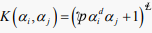 ,
,  (Polynomial) (9)
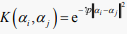 ,
,  (RBF or Gaussian) (10)