

Paper Menu >>
Journal Menu >>
 iBusiness, 2011, 3, 383-389 doi:10.4236/ib.2011.34051 Published Online December 2011 (http://www.SciRP.org/journal/ib) Copyright © 2011 SciRes. IB 383 Ordinal Logistic Regression for the Estimate of the Response Functions in the Conjoint Analysis Amedeo De Luca Dipartimento di Scienze Statistiche, Università Cattolica del Sacro Cuore di Milano, Milan, Italy. Email: [email protected] Received June 28th, 2011; revised August 29th, 2011; accepted September 28th, 2011. ABSTRACT In the Conjoint Analysis (COA) model proposed here—a new approach to estimate more than one response function— an extension of the traditional COA, the polytomous response variable (i.e. evaluation of th e overall desirability of al- ternative product profiles) is described by a sequence of binary variables. To link the categories of overall evaluation to the factor levels, we adopt—at the aggregate level—an ordinal logistic regression, based on a main effects experimen- tal design. The model provides several overall desirability functions (aggregated part-worths sets), as many as the overall ordered categories are, unlike the traditiona l metric and non metric COA, which gives only one response func- tion. We provide an application of the model and an interpretation of the main effects. Keywords: Aggregate Level Analysis, Conjoint Analysis, Ordinal Logistic Regression, Respon se Fun c t i on 1. Introduction Since the 1970s, Conjoint Analysis (COA) has received considerable attention as a major set of techniques for measuring buyers’ trade-offs among multiattributed pro- ducts and services [1]. Since that time many new developments in COA have been reported. The purpose of this article is to give a new contri- bution to the problem of the conjoint measurement in order to quantify judgmental data. The model proposed here is an extension of the tradi- tional COA approach. While in the traditional full-profile COA [1] the re- spondent expresses preferences by rating or ranking distinct product profiles, in our model we assume that the re- spondent evaluative judgement Yk on the overall desir- ability consists in a choice of one of the k (k = 1, 2, ···, K) desirability categories for each of S hypothetical product profiles, chosen from a sample of respondents. The proposed approach also differs from the “Choice-Based Conjoint” analysis (CBC) model in which the respondent expresses preferences by choos- ing concepts from sets of concepts (discrete choice modelling). In the proposed approach the ordinal response variable is described by an ordered logit model, that directly in- corporates the order of the categories of the Yk. To link the categories of overall evaluation to the fac- tor levels, we adopt a cumulative logit model [2] at the aggregate level (pooled model) [3]. The main novelty value in our approach—which is a further development—is that one set of aggregated part- worths is estimated in connection with each category Yk, as many as the overall ordered categories are (K), unlike the traditional metric and non metric COA and CBC analysis, which give only one set of aggregated part- worths (response function). Thus with our approach it is possible to make a cross-check of the effects of the attribute levels on the different k categories of Yk. Moreover, the proposed model provides the following advantages: the use of the probability Pks as an average response, which does not require preliminary scale ad- justments to render the preference scale “metric” (in the non metric COA) and a cross-check of the effects of the attribute levels on the different categories of the overall. This allows us to verify the basic coherence of the re- sults of the model, unlike the classical approach adopted in literature. This paper is structured as follows: after the presen- tation of the proposed model and the estimation method of response functions (the cumulative logit model), a concrete application of the approach follows; then the meaning of the proposed interpretative model and some empirical results are described, to conclude with a 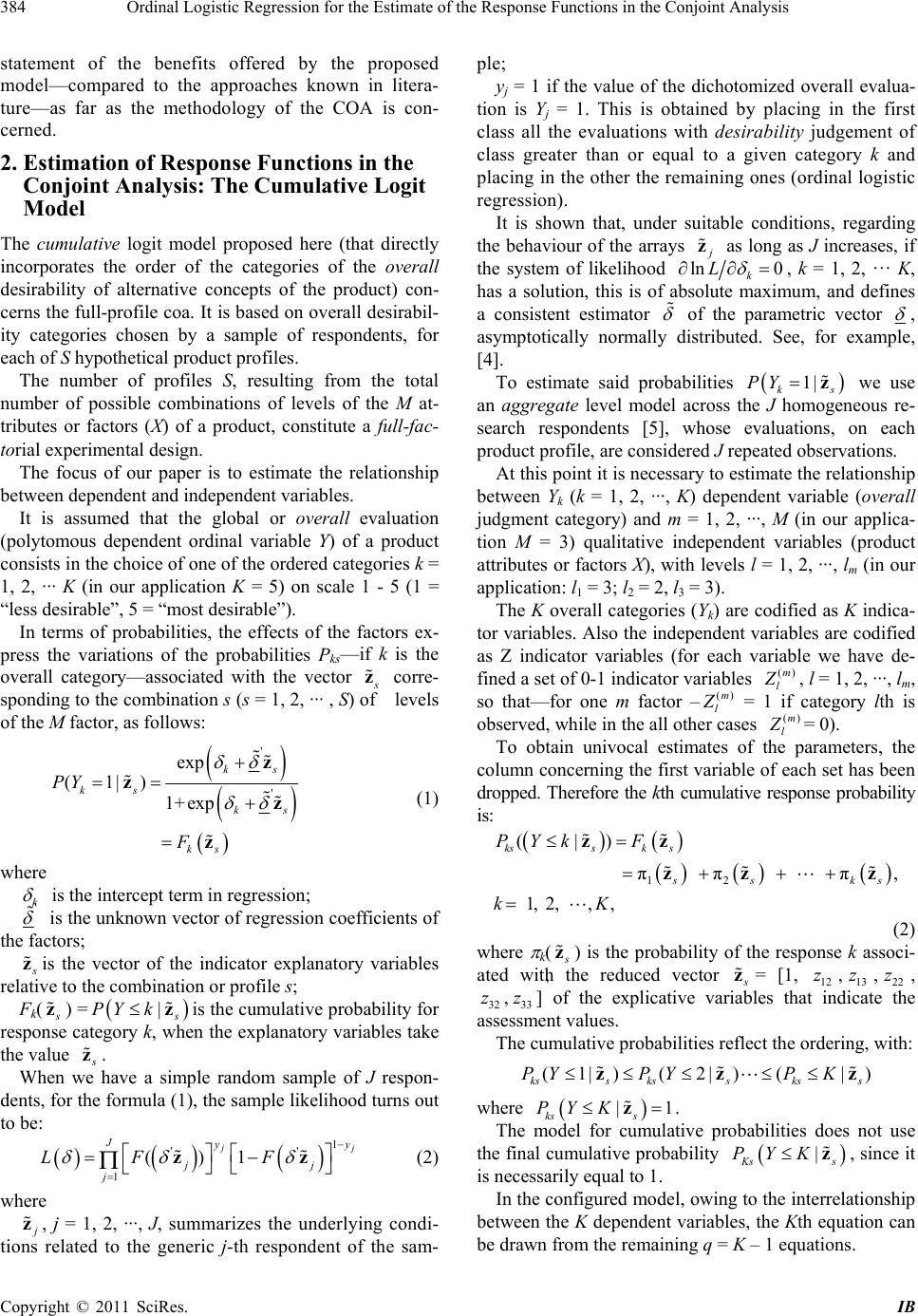 Ordinal Logistic Regression for the Estimate of the Response Functions in the Conjoint Analysis 384 statement of the benefits offered by the proposed model—compared to the approaches known in litera- ture—as far as the methodology of the COA is con- cerned. 2. Estimation of Response Functions in the Conjoint Analysis: The Cumulative Logit Model The cumulative logit model proposed here (that directly incorporates the order of the categories of the overall desirability of alternative concepts of the product) con- cerns the full-profile coa. It is based on overall desirabil- ity categories chosen by a sample of respondents, for each of S hypothetical product profiles. The number of profiles S, resulting from the total number of possible combinations of levels of the M at- tributes or factors (X) of a product, constitute a full-fac- torial experimental design. The focus of our paper is to estimate the relationship between dependent and independent variables. It is assumed that the global or overall evaluation (polytomous dependent ordinal variable Y) of a product consists in the choice of one of the ordered categories k = 1, 2, ··· K (in our application K = 5) on scale 1 - 5 (1 = “less desirable”, 5 = “most desirable”). In terms of probabilities, the effects of the factors ex- press the variations of the probabilities Pks—if k is the overall category—associated with the vector s z corre- sponding to the combination s (s = 1, 2, ··· , S) of levels of the M factor, as follows: ' ' exp (1|) 1+ exp ks ks ks ks PY F z zz z (1) where k is the intercept term in regression; ' is the unknown vector of regression coefficients of the factors; s z is the vector of the indicator explanatory variables relative to the combination or profile s; Fk( s z) = | s PY kz is the cumulative probability for response category k, when the explanatory variables take the value s z . When we have a simple random sample of J respon- dents, for the formula (1), the sample likelihood turns out to be: 1 '' 1 ()1 j j Jyy j j LF F zz j (2) where j z , j = 1, 2, ···, J, summarizes the underlying condi- tions related to the generic j-th respondent of the sam- ple; yj = 1 if the value of the dichotomized overall evalua- tion is Yj = 1. This is obtained by placing in the first class all the evaluations with desirability judgement of class greater than or equal to a given category k and placing in the other the remaining ones (ordinal logistic regression). It is shown that, under suitable conditions, regarding the behaviour of the arrays j z as long as J increases, if the system of likelihood ln L0 k , k = 1, 2, … K, has a solution, this is of absolute maximum, and defines a consistent estimator of the parametric vector , asymptotically normally distributed. See, for example, [4]. To estimate said probabilities s we use an aggregate level model across the J homogeneous re- search respondents [5], whose evaluations, on each product profile, are considered J repeated observations. 1| k PYz At this point it is necessary to estimate the relationship between Yk (k = 1, 2, ···, K) dependent variable (overall judgment category) and m = 1, 2, ..., M (in our applica- tion M = 3) qualitative independent variables (product attributes or factors X), with levels l = 1, 2, ···, lm (in our application: l1 = 3; l2 = 2, l3 = 3). The K overall categories (Yk) are codified as K indica- tor variables. Also the independent variables are codified as Z indicator variables (for each variable we have de- fined a set of 0-1 indicator variables ()m l Z , l = 1, 2, ···, lm, so that—for one m factor –()m l Z = 1 if category lth is observed, while in the all other cases ()m l Z = 0). To obtain univocal estimates of the parameters, the column concerning the first variable of each set has been dropped. Therefore the kth cumulative response probability is: 12 (|) π π π, 1, 2, ,, kssk s ss k PYk F kK zz zz z s (2) where k( s z) is the probability of the response k associ- ated with the reduced vector s z = [1, 12 ,13 ,22 , 32 ,33 ]'of the explicative variables that indicate the assessment values. zzz z z The cumulative probabilities reflect the ordering, with: (1|)( 2|)(| kss ksskss PYPYP K) zz z where |1 ks s PY K z . The model for cumulative probabilities does not use the final cumulative probability | K s PYKz s , since it is necessarily equal to 1. In the configured model, owing to the interrelationship between the K dependent variables, the Kth equation can be drawn from the remaining q = K – 1 equations. Copyright © 2011 SciRes. IB 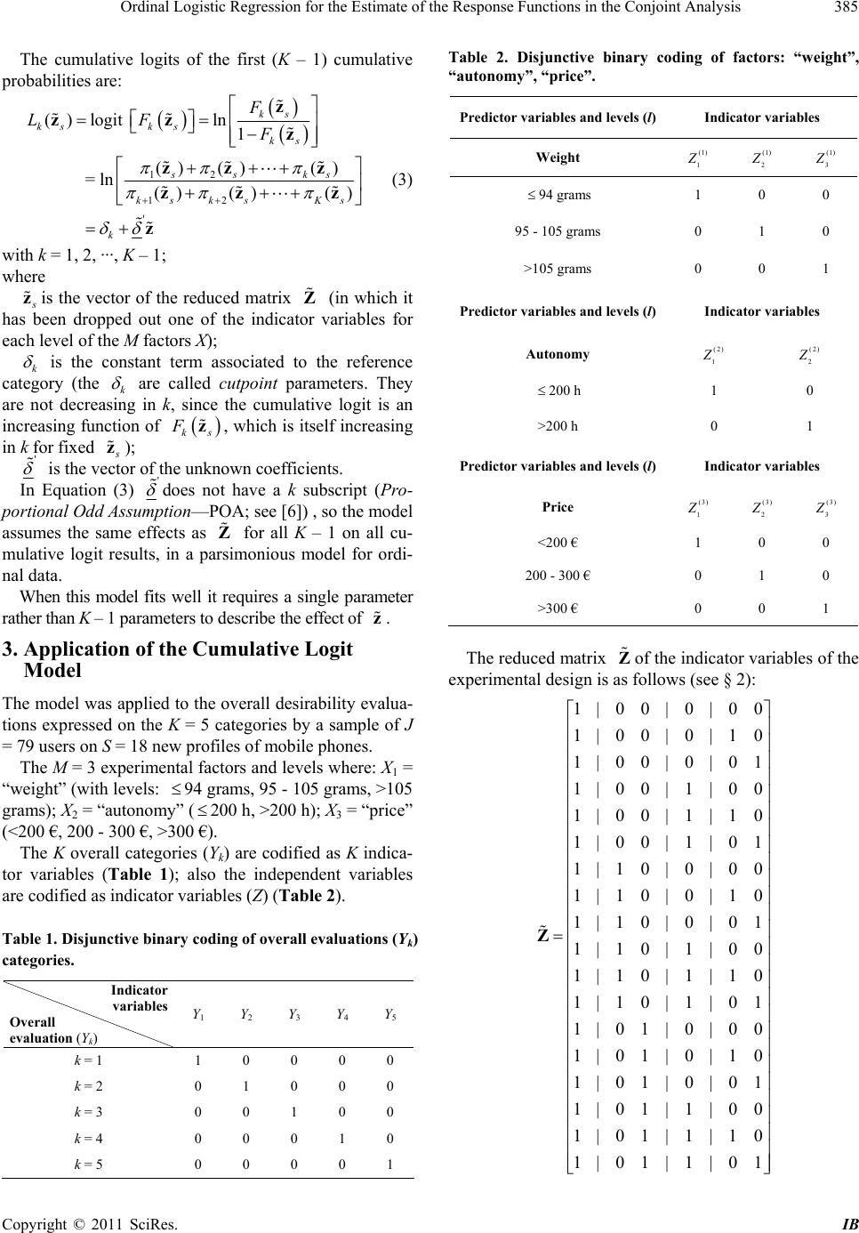 Ordinal Logistic Regression for the Estimate of the Response Functions in the Conjoint Analysis385 The cumulative logits of the first (K – 1) cumulative probabilities are: 12 12 ' ()logit ln1 () ()() = ln() ()() ks ksk sks ss ks ksk sKs k F LF F z zz z zz z zz z z (3) with k = 1, 2, ···, K – 1; where s z is the vector of the reduced matrix (in which it has been dropped out one of the indicator variables for each level of the M factors X); Z k is the constant term associated to the reference category (the k are called cutpoint parameters. They are not decreasing in k, since the cumulative logit is an increasing function of , which is itself increasing in k for fixed ks Fz s z ); ' is the vector of the unknown coefficients. In Equation (3) ' does not have a k subscript (Pro- portional Odd Assumption—POA; see [6]) , so the model assumes the same effects as for all K – 1 on all cu- mulative logit results, in a parsimonious model for ordi- nal data. Z When this model fits well it requires a single parameter rather than K – 1 parameters to describe the effect of . z 3. Application of the Cumulative Logit Model The model was applied to the overall desirability evalua- tions expressed on the K = 5 categories by a sample of J = 79 users on S = 18 new profiles of mobile phones. The M = 3 experimental factors and levels where: X1 = “weight” (with levels: 94 grams, 95 - 105 grams, >105 grams); X2 = “autonomy” (200 h, >200 h); X3 = “price” (<200 €, 200 - 300 €, >300 €). The K overall categories (Yk) are codified as K indica- tor variables (Table 1); also the independent variables are codified as indicator variables (Z) (Table 2). Table 1. Disjunctive binary coding of overall evaluations (Yk) categories. Indicator variables Overall evaluation (Yk) Y1 Y2 Y3 Y4 Y 5 k = 1 1 0 0 0 0 k = 2 0 1 0 0 0 k = 3 0 0 1 0 0 k = 4 0 0 0 1 0 k = 5 0 0 0 0 1 Table 2. Disjunctive binary coding of factors: “weight”, “autonomy”, “price”. Predictor variables and levels (l) Indicator variables Weight (1) 1 Z (1) 2 Z (1) 3 Z 94 grams 1 0 0 95 - 105 grams 0 1 0 >105 grams 0 0 1 Predictor variables and levels (l) Indicator variables Autonomy (2) 1 Z (2) 2 Z 200 h 1 0 >200 h 0 1 Predictor variables and levels (l) Indicator variables Price (3) 1 Z (3) 2 Z (3) 3 Z <200 € 1 0 0 200 - 300 € 0 1 0 >300 € 0 0 1 The reduced matrix of the indicator variables of the experimental design is as follows (see § 2): Z 1| 0 0|0 |00 1| 0 0|0 |10 1| 0 0|0 |01 1|00|1|00 1|00|1|10 1|00|1|01 1|1 0|0| 0 0 1|1 0|0|1 0 1|1 0| 0| 0 1 1|10|1|00 1|10|1|10 1|10|1|01 1| 0 1| 0| 0 0 1| 0 1| 0| 1 0 1| 0 1| 0| 0 1 1| 0 1|1| 0 0 1|0 1|1|10 1| 0 1|1| 0 1 Z Copyright © 2011 SciRes. IB 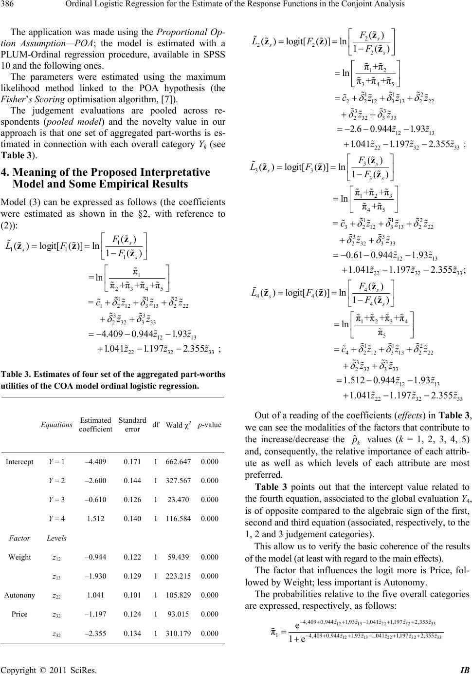 Ordinal Logistic Regression for the Estimate of the Response Functions in the Conjoint Analysis 386 The application was made using the Proportional Op- tion Assumption—POA; the model is estimated with a PLUM-Ordinal regression procedure, available in SPSS 10 and the following ones. The parameters were estimated using the maximum likelihood method linked to the POA hypothesis (the Fisher’s Scori ng optimisation algorithm, [7]). The judgement evaluations are pooled across re- spondents (pooled model) and the novelty value in our approach is that one set of aggregated part-worths is es- timated in connection with each overall category Yk (see Table 3). 4. Meaning of the Proposed Interpretative Model and Some Empirical Results Model (3) can be expressed as follows (the coefficients were estimated as shown in the §2, with reference to (2)): 1 11 1 1 2345 112 12 12313222 () ()logit[()] ln1() π =lnπ+π+π+π = s ss F LF F cz zz z zz z 33 232 333 12 13 22 3233 4.4090.9441.93 1.0411.1972.355 ; zz zz zzz Table 3. Estimates of four set of the aggregated part-worths utilities of the COA model ordinal logistic regression. Equations Estimated coefficient Standard error df Wald 2p-value Intercept Y = 1 –4.409 0.171 1 662.6470.000 Y = 2 –2.600 0.144 1 327.5670.000 Y = 3 –0.610 0.126 1 23.4700.000 Y = 4 1.512 0.140 1 116.5840.000 Factor Levels Weight z12 –0.944 0.122 1 59.4390.000 z13 –1.930 0.129 1 223.2150.000 Autonony z22 1.041 0.101 1 105.8290.000 Price z32 –1.197 0.124 1 93.0150.000 z32 –2.355 0.134 1 310.1790.000 2 22 2 12 345 112 22 123 13222 () ()logit[()] ln1() π+π lnπ+π+π s ss F LF F cz zz z zz z 33 232 333 12 13 22 3233 2.60.9441.93 1.0411.1972.355 ; zz zz zz z 3 33 3 123 45 112 3 212 313 222 () () logit[ ()] ln1() π+π+π lnπ+π = s ss F LF F cz zz z zz z 33 232333 12 13 22 3233 0.610.9441.93 1.0411.1972.355; zz zz zz z 4 44 4 1234 5 112 42 12313222 () ()logit[()] ln1() π+π+π+π lnπ s ss F LF F cz zz z zz z 33 232 333 12 13 22 3233 1.5120.9441.93 1.0411.1972.355 zz zz zz z Out of a reading of the coefficients (effects) in Tabl e 3 , we can see the modalities of the factors that contribute to the increase/decrease the values (k = 1, 2, 3, 4, 5) and, consequently, the relative importance of each attrib- ute as well as which levels of each attribute are most preferred. ˆk p Table 3 points out that the intercept value related to the fourth equation, associated to the global evaluation Y4, is of opposite compared to the algebraic sign of the first, second and third equation (associated, respectively, to the 1, 2 and 3 judgement categories). This allow us to verify the basic coherence of the results of the model (at least with regard to the main effects). The factor that influences the logit more is Price, fol- lowed by Weight; less important is Autonomy. The probabilities relative to the five overall categories are expressed, respectively, as follows: 12 13223233 12 13223233 4,409 0,9441,931,0411,1972,355 14,409 0,9441,931,0411,1972,355 e π 1e zz zzz z zzzz Copyright © 2011 SciRes. IB 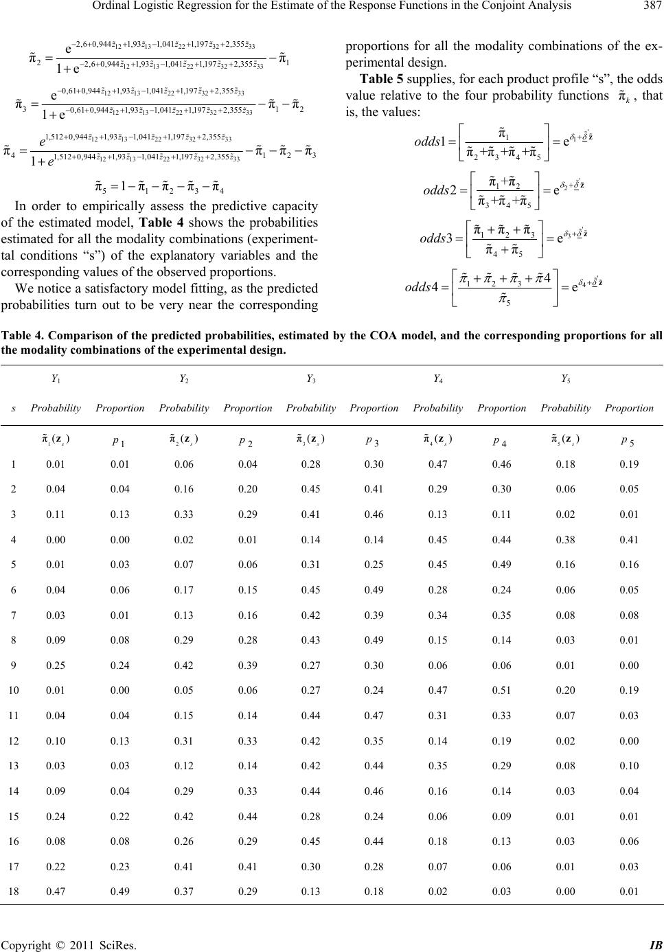 Ordinal Logistic Regression for the Estimate of the Response Functions in the Conjoint Analysis Copyright © 2011 SciRes. IB 387 12 13223233 12 13223233 2,6 0,9441,931,0411,1972,355 21 2,6 0,9441,931,0411,1972,355 e ππ 1e zz zzz zz zzz 12 13223233 12 13223233 0,61 0,9441,931,0411,1972,355 31 0,61 0,9441,931,0411,1972,355 e π 1e zz zzz zz zzz 2 π π 12 13223233 12 13223233 1,5120,9441,931,0411,1972,355 4123 π 1,5120,9441,931,0411,1972,355 πππ 1 zz zzz zz zzz e e 4 5123 π1ππ ππ In order to empirically assess the predictive capacity of the estimated model, Table 4 shows the probabilities estimated for all the modality combinations (experiment- tal conditions “s”) of the explanatory variables and the corresponding values of the observed proportions. We notice a satisfactory model fitting, as the predicted probabilities turn out to be very near the corresponding proportions for all the modality combinations of the ex- perimental design. Table 5 supplies, for each product profile “s”, the odds value relative to the four probability functions , that is, the values: πk ' 1 1 2345 π 1e π+π+π+π odds z ' 2 12 345 π+π 2e π+π+π odds z ' 3 123 45 ππ π 3e ππ odds z ' 4 123 5 4 4e odds z Table 4. Comparison of the predicted probabilities, estimated by the COA model, and the corresponding proportions for all the modality combinations of the experimental design. Y 1 Y 2 Y 3 Y 4 Y 5 s Probability Proportion Probability ProportionProbabilityProportionProbabilityProportion Probability Proportion 1 π() s z p1 2 π() s z p 23 π() s z p 34 π() s z p 45 π() s z p 5 1 0.01 0.01 0.06 0.04 0.28 0.30 0.47 0.46 0.18 0.19 2 0.04 0.04 0.16 0.20 0.45 0.41 0.29 0.30 0.06 0.05 3 0.11 0.13 0.33 0.29 0.41 0.46 0.13 0.11 0.02 0.01 4 0.00 0.00 0.02 0.01 0.14 0.14 0.45 0.44 0.38 0.41 5 0.01 0.03 0.07 0.06 0.31 0.25 0.45 0.49 0.16 0.16 6 0.04 0.06 0.17 0.15 0.45 0.49 0.28 0.24 0.06 0.05 7 0.03 0.01 0.13 0.16 0.42 0.39 0.34 0.35 0.08 0.08 8 0.09 0.08 0.29 0.28 0.43 0.49 0.15 0.14 0.03 0.01 9 0.25 0.24 0.42 0.39 0.27 0.30 0.06 0.06 0.01 0.00 10 0.01 0.00 0.05 0.06 0.27 0.24 0.47 0.51 0.20 0.19 11 0.04 0.04 0.15 0.14 0.44 0.47 0.31 0.33 0.07 0.03 12 0.10 0.13 0.31 0.33 0.42 0.35 0.14 0.19 0.02 0.00 13 0.03 0.03 0.12 0.14 0.42 0.44 0.35 0.29 0.08 0.10 14 0.09 0.04 0.29 0.33 0.44 0.46 0.16 0.14 0.03 0.04 15 0.24 0.22 0.42 0.44 0.28 0.24 0.06 0.09 0.01 0.01 16 0.08 0.08 0.26 0.29 0.45 0.44 0.18 0.13 0.03 0.06 17 0.22 0.23 0.41 0.41 0.30 0.28 0.07 0.06 0.01 0.03 18 0.47 0.49 0.37 0.29 0.13 0.18 0.02 0.03 0.00 0.01 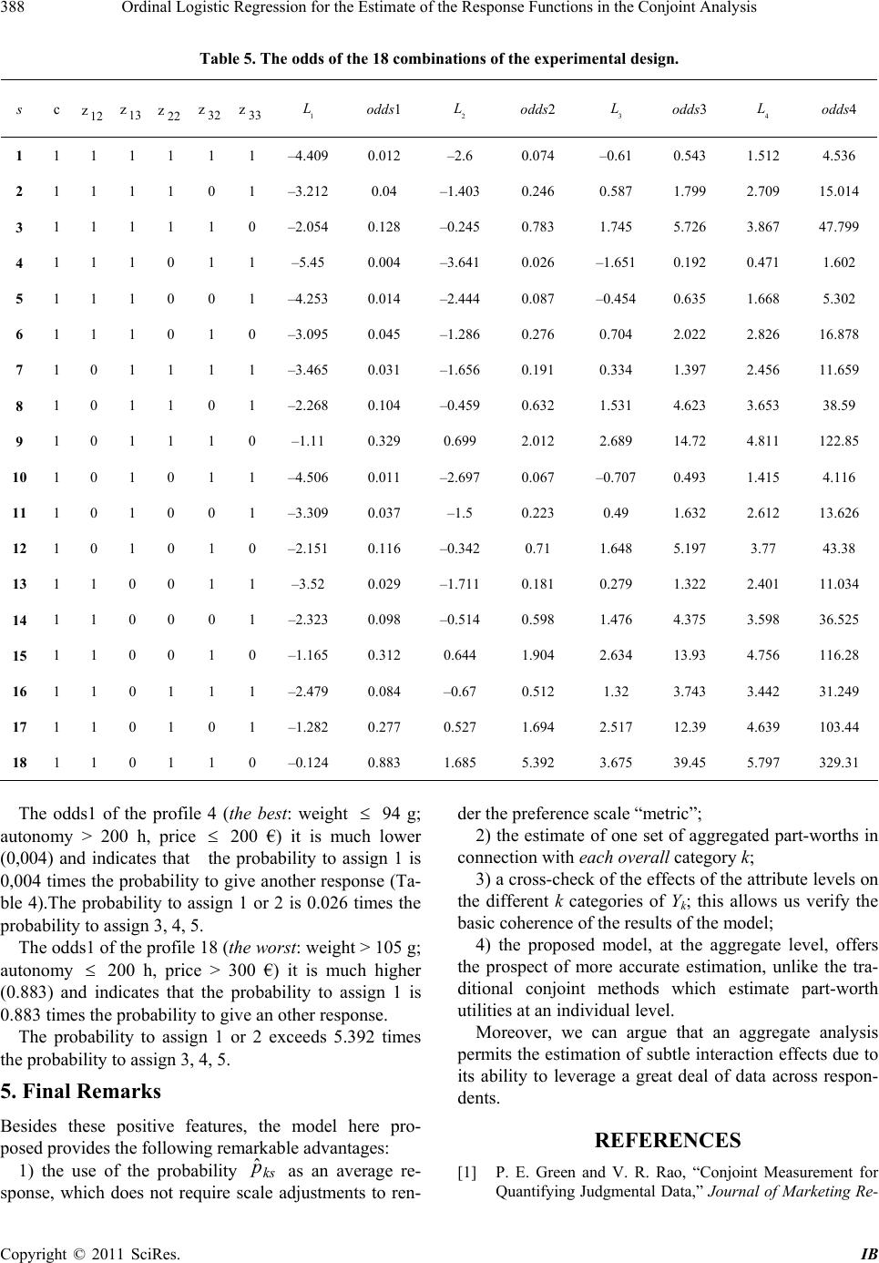 Ordinal Logistic Regression for the Estimate of the Response Functions in the Conjoint Analysis 388 Table 5. The odds of the 18 combinations of the experimental design. s c z 12 z 13 z 22 z32 z 33 1 L odds1 2 L odds2 3 L odds3 4 L odds4 1 1 1 1 1 1 1 –4.409 0.012 –2.6 0.074 –0.61 0.543 1.512 4.536 2 1 1 1 1 0 1 –3.212 0.04 –1.403 0.246 0.587 1.799 2.709 15.014 3 1 1 1 1 1 0 –2.054 0.128 –0.245 0.783 1.745 5.726 3.867 47.799 4 1 1 1 0 1 1 –5.45 0.004 –3.641 0.026 –1.651 0.192 0.471 1.602 5 1 1 1 0 0 1 –4.253 0.014 –2.444 0.087 –0.454 0.635 1.668 5.302 6 1 1 1 0 1 0 –3.095 0.045 –1.286 0.276 0.704 2.022 2.826 16.878 7 1 0 1 1 1 1 –3.465 0.031 –1.656 0.191 0.334 1.397 2.456 11.659 8 1 0 1 1 0 1 –2.268 0.104 –0.459 0.632 1.531 4.623 3.653 38.59 9 1 0 1 1 1 0 –1.11 0.329 0.699 2.012 2.689 14.72 4.811 122.85 10 1 0 1 0 1 1 –4.506 0.011 –2.697 0.067 –0.707 0.493 1.415 4.116 11 1 0 1 0 0 1 –3.309 0.037 –1.5 0.223 0.49 1.632 2.612 13.626 12 1 0 1 0 1 0 –2.151 0.116 –0.342 0.71 1.648 5.197 3.77 43.38 13 1 1 0 0 1 1 –3.52 0.029 –1.711 0.181 0.279 1.322 2.401 11.034 14 1 1 0 0 0 1 –2.323 0.098 –0.514 0.598 1.476 4.375 3.598 36.525 15 1 1 0 0 1 0 –1.165 0.312 0.644 1.904 2.634 13.93 4.756 116.28 16 1 1 0 1 1 1 –2.479 0.084 –0.67 0.512 1.32 3.743 3.442 31.249 17 1 1 0 1 0 1 –1.282 0.277 0.527 1.694 2.517 12.39 4.639 103.44 18 1 1 0 1 1 0 –0.124 0.883 1.685 5.392 3.675 39.45 5.797 329.31 The odds1 of the profile 4 (the best: weight 94 g; autonomy > 200 h, price 200 €) it is much lower (0,004) and indicates that the probability to assign 1 is 0,004 times the probability to give another response (Ta- ble 4).The probability to assign 1 or 2 is 0.026 times the probability to assign 3, 4, 5. The odds1 of the profile 18 (the worst: weight > 105 g; autonomy 200 h, price > 300 €) it is much higher (0.883) and indicates that the probability to assign 1 is 0.883 times the probability to give an other response. The probability to assign 1 or 2 exceeds 5.392 times the probability to assign 3, 4, 5. 5. Final Remarks Besides these positive features, the model here pro- posed provides the following remarkable advantages: 1) the use of the probability as an average re- sponse, which does not require scale adjustments to ren- der the preference scale “metric”; ks p ˆ 2) the estimate of one set of aggregated part-worths in connection with each overall category k; 3) a cross-check of the effects of the attribute levels on the different k categories of Yk; this allows us verify the basic coherence of the results of the model; 4) the proposed model, at the aggregate level, offers the prospect of more accurate estimation, unlike the tra- ditional conjoint methods which estimate part-worth utilities at an individual level. Moreover, we can argue that an aggregate analysis permits the estimation of subtle interaction effects due to its ability to leverage a great deal of data across respon- dents. REFERENCES [1] P. E. Green and V. R. Rao, “Conjoint Measurement for Quantifying Judgmental Data,” Journal of Marketing Re- Copyright © 2011 SciRes. IB  Ordinal Logistic Regression for the Estimate of the Response Functions in the Conjoint Analysis389 search, Vol. 8, No. 3, 1971, pp. 355-363. [2] A. De Luca, “A Logit Model with a Variable Response and Predictors on an Ordinal Scale to Measure Customer Satisfaction,” Quality and Reliability Engineering Inter- national, Vol. 22, No. 5, 2006, pp. 591-602. doi:10.1002/qre.764 [3] W. L. Moore, “Levels of Aggregation in Conjoint Analy- sis: An Empirical Comparison,” Journal of Marketing Research, Vol. 17, No. 4, 1980, pp. 516-523. doi:10.2307/3150504 [4] T. Amemiya, “Advanced Econometrics,” Blackwell Ltd., Oxford, 1985. [5] A. De Luca and S. Ciapparelli, “Multivariate Logistic Re- gression for the Estimate of Response Functions in the Conjoint Analysis,” Proceedings MTISD 2008—Methods, Models and Information Technologies for Decision Sup- port Systems, Università del Salento, Lecce, 2008, pp. 23-24. [6] B. Peterson and F. E. Harrell, “Partial Proportional Odds Models for Ordinal Response Variables,” Applied Statis- tics, Vol. 39, No. 2, 1990, pp. 205-207. doi:10.2307/2347760 [7] P. McCullagh, “Regression Models for Ordinal Data,” Journal of Royal Statistical Society, Vol. 42, No. 2, 1980, pp. 109-142. Copyright © 2011 SciRes. IB |