Principal Component Analyses in Anthropological Genetics

doi:10.4236/aa.2011.12002

Paper Menu >>

Journal Menu >>

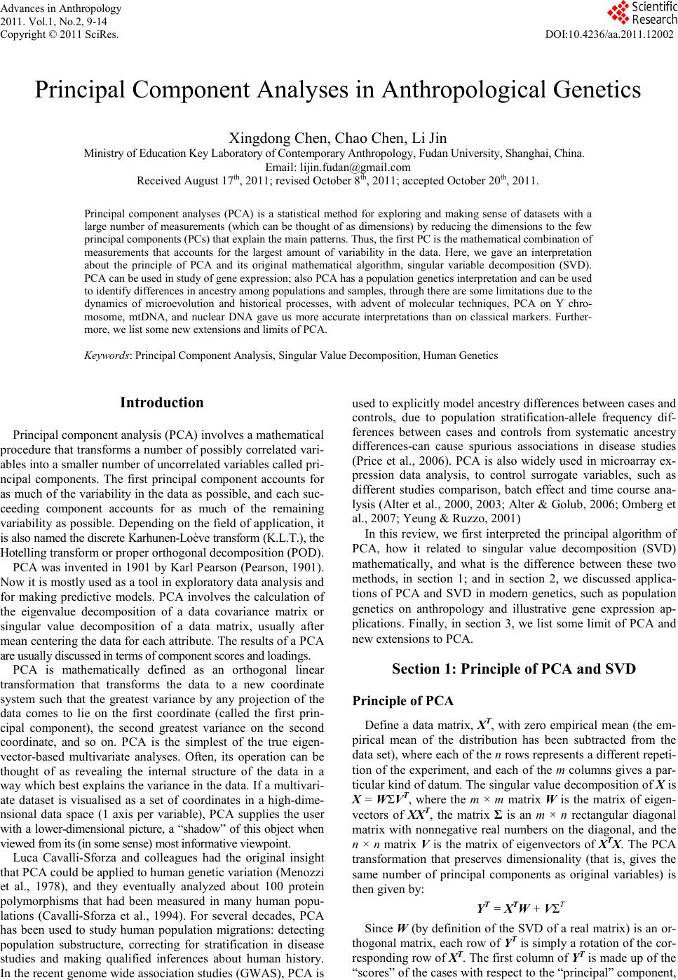Advances in Anthropology

2011. Vol.1, No.2, 9-14

Principal Component Analyses in Anthropological Genetics

Xingdong Chen, Chao Chen, Li Jin

Ministry of Education Key Laboratory of Contemporary Anthropology, Fudan University, Shanghai, China.

Email: [email protected]

Received August 17th, 2011; revised October 8th, 2011; accepted October 20th, 2011.

Principal component analyses (PCA) is a statistical method for exploring and making sense of datasets with a

large number of measurements (which can be thought of as dimensions) by reducing the dimensions to the few

principal components (PCs) that explain the main patterns. Thus, the first PC is the mathematical combination of

measurements that accounts for the largest amount of variability in the data. Here, we gave an interpretation

about the principle of PCA and its original mathematical algorithm, singular variable decomposition (SVD).

PCA can be used in study of gene expression; also PCA has a population genetics interpretation and can be used

to identify differences in ancestry among populations and samples, through there are some limitations due to the

dynamics of microevolution and historical processes, with advent of molecular techniques, PCA on Y chro-

mosome, mtDNA, and nuclear DNA gave us more accurate interpretations than on classical markers. Further-

more, we list some new extensions and limits of PCA.

Keywords: Principal Component Analysis, Singular Value Decomposition, Human Genetics

Introduction

Principal component analysis (PCA) involves a mathematical

procedure that transforms a number of possibly correlated vari-

ables into a smaller number of uncorrelated variables called pri-

ncipal components. The first principal component accounts for

as much of the variability in the data as possible, and each suc-

ceeding component accounts for as much of the remaining

variability as possible. Depending on the field of application, it

is also named the discrete Karhunen-Loève transform (K.L.T.), the

Hotelling transform or proper orthogonal decomposition (POD).

PCA was invented in 1901 by Karl Pearson (Pearson, 1901).

Now it is mostly used as a tool in exploratory data analysis and

for making predictive models. PCA involves the calculation of

the eigenvalue decomposition of a data covariance matrix or

singular value decomposition of a data matrix, usually after

mean centering the data for each attribute. The results of a PCA

are usually discussed in terms of component scores and loadings.

PCA is mathematically defined as an orthogonal linear

transformation that transforms the data to a new coordinate

system such that the greatest variance by any projection of the

data comes to lie on the first coordinate (called the first prin-

cipal component), the second greatest variance on the second

coordinate, and so on. PCA is the simplest of the true eigen-

vector-based multivariate analyses. Often, its operation can be

thought of as revealing the internal structure of the data in a

way which best explains the variance in the data. If a multivari-

ate dataset is visualised as a set of coordinates in a high-dime-

nsional data space (1 axis per variable), PCA supplies the user

with a lower-dimensional picture, a “shadow” of this object when

viewed from its (in some sense) most informative viewpoint.

Luca Cavalli-Sforza and colleagues had the original insight

that PCA could be applied to human genetic variation (Menozzi

et al., 1978), and they eventually analyzed about 100 protein

polymorphisms that had been measured in many human popu-

lations (Cavalli-Sforza et al., 1994). For several decades, PCA

has been used to study human population migrations: detecting

population substructure, correcting for stratification in disease

studies and making qualified inferences about human history.

In the recent genome wide association studies (GWAS), PCA is

used to explicitly model ancestry differences between cases and

controls, due to population stratification-allele frequency dif-

ferences between cases and controls from systematic ancestry

differences-can cause spurious associations in disease studies

(Price et al., 2006). PCA is also widely used in microarray ex-

pression data analysis, to control surrogate variables, such as

different studies comparison, batch effect and time course ana-

lysis (Alter et al., 2000, 2003; Alter & Golub, 2006; Omberg et

al., 2007; Yeung & Ruzzo, 2001)

In this review, we first interpreted the principal algorithm of

PCA, how it related to singular value decomposition (SVD)

mathematically, and what is the difference between these two

methods, in section 1; and in section 2, we discussed applica-

tions of PCA and SVD in modern genetics, such as population

genetics on anthropology and illustrative gene expression ap-

plications. Finally, in section 3, we list some limit of PCA and

new extensions to PCA.

Section 1: Principle of PCA and SVD

Principle of PCA

Define a data matrix, XT, with zero empirical mean (the em-

pirical mean of the distribution has been subtracted from the

data set), where each of the n rows represents a different repeti-

tion of the experiment, and each of the m columns gives a par-

ticular kind of datum. The singular value decomposition of X is

X = WΣVT, where the m × m matrix W is the matrix of eigen-

vectors of XXT, the matrix Σ is an m × n rectangular diagonal

matrix with nonnegative real numbers on the diagonal, and the

n × n matrix V is the matrix of eigenvectors of XTX. The PCA

transformation that preserves dimensionality (that is, gives the

same number of principal components as original variables) is

then given by:

YT = XTW + VΣT

Since W (by definition of the SVD of a real matrix) is an or-

thogonal matrix, each row of YT is simply a rotation of the cor-

responding row of XT. The first column of YT is made up of the

“scores” of the cases with respect to the “principal” component,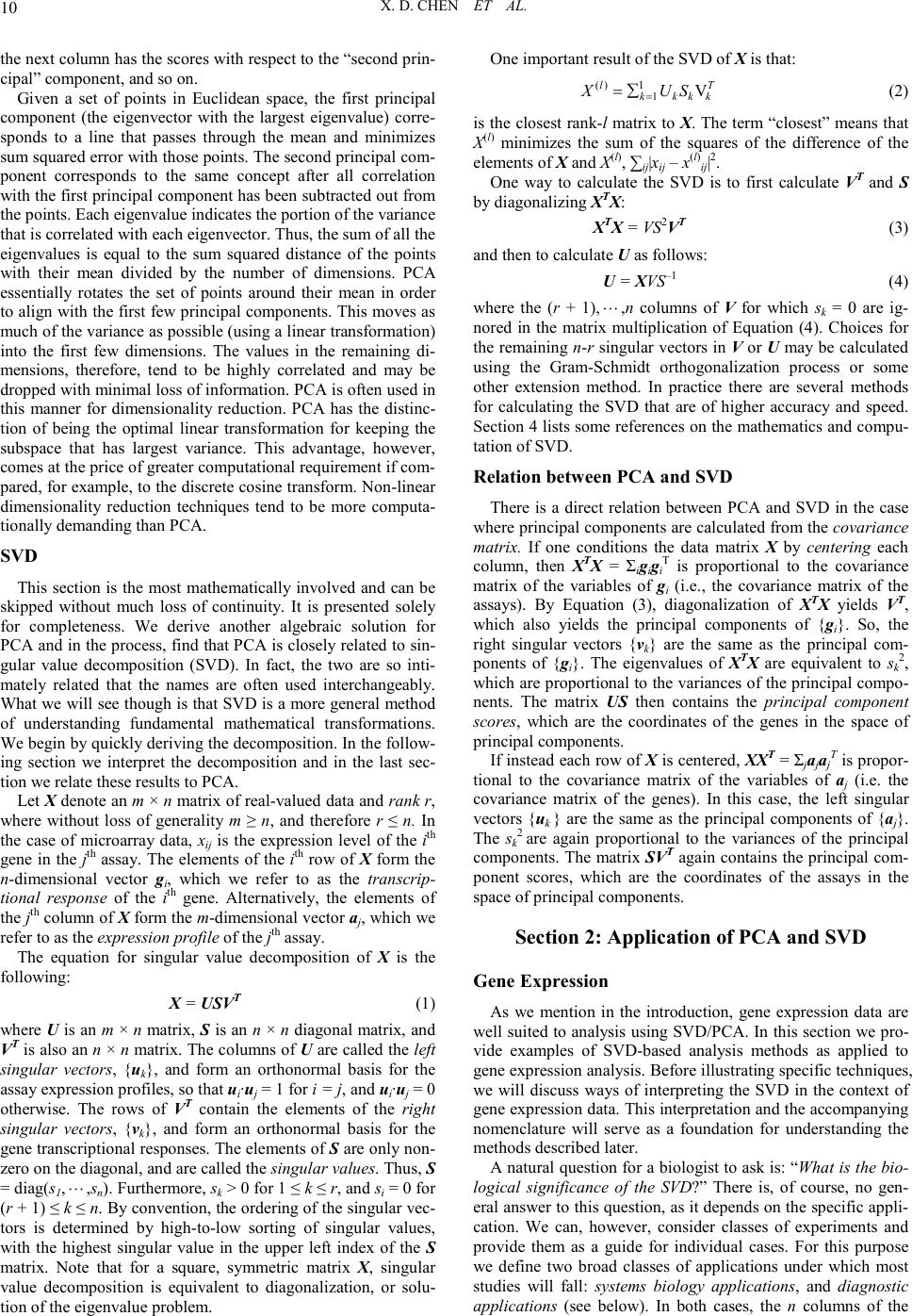

X. D. CHEN ET AL.

the next column has the scores with respect to the “second prin-

cipal” component, and so on.

Given a set of points in Euclidean space, the first principal

component (the eigenvector with the largest eigenvalue) corre-

sponds to a line that passes through the mean and minimizes

sum squared error with those points. The second principal com-

ponent corresponds to the same concept after all correlation

with the first principal component has been subtracted out from

the points. Each eigenvalue indicates the portion of the variance

that is correlated with each eigenvector. Thus, the sum of all the

eigenvalues is equal to the sum squared distance of the points

with their mean divided by the number of dimensions. PCA

essentially rotates the set of points around their mean in order

to align with the first few principal components. This moves as

much of the variance as possible (using a linear transformation)

into the first few dimensions. The values in the remaining di-

mensions, therefore, tend to be highly correlated and may be

dropped with minimal loss of information. PCA is often used in

this manner for dimensionality reduction. PCA has the distinc-

tion of being the optimal linear transformation for keeping the

subspace that has largest variance. This advantage, however,

comes at the price of greater computational requirement if com-

pared, for example, to the discrete cosine transform. Non-linear

dimensionality reduction techniques tend to be more computa-

tionally demanding than PCA.

SVD

This section is the most mathematically involved and can be

skipped without much loss of continuity. It is presented solely

for completeness. We derive another algebraic solution for

PCA and in the process, find that PCA is closely related to sin-

gular value decomposition (SVD). In fact, the two are so inti-

mately related that the names are often used interchangeably.

What we will see though is that SVD is a more general method

of understanding fundamental mathematical transformations.

We begin by quickly deriving the decomposition. In the follow-

ing section we interpret the decomposition and in the last sec-

tion we relate these results to PCA.

Let X denote an m × n matrix of real-valued data and rank r,

where without loss of generality m ≥ n, and therefore r ≤ n. In

the case of microarray data, xij is the expression level of the ith

gene in the jth assay. The elements of the ith row of X form the

n-dimensional vector gi, which we refer to as the transcrip-

tional response of the ith gene. Alternatively, the elements of

the jth column of X form the m-dimensional vector aj, which we

refer to as the expre s si on profile of the jth assay.

The equation for singular value decomposition of X is the

following:

X = USVT (1)

where U is an m × n matrix, S is an n × n diagonal matrix, and

VT is also an n × n matrix. The columns of U are called the left

singular vectors, {uk}, and form an orthonormal basis for the

assay expression profiles, so that ui·uj = 1 for i = j, and ui·uj = 0

otherwise. The rows of VT contain the elements of the right

singular vectors, {vk}, and form an orthonormal basis for the

gene transcriptional responses. The elements of S are only non-

zero on the diagonal, and are called the singular values. Thus, S

= diag(s1,,sn). Furthermore, sk > 0 for 1 ≤ k ≤ r, and si = 0 for

(r + 1) ≤ k ≤ n. By convention, the ordering of the singular vec-

tors is determined by high-to-low sorting of singular values,

with the highest singular value in the upper left index of the S

matrix. Note that for a square, symmetric matrix X, singular

value decomposition is equivalent to diagonalization, or solu-

tion of the eigenvalue problem.

One important result of the SVD of X is that:

() 1

kkkk

XUS



 T

(2)

is the closest rank-l matrix to X. The term “closest” means that

X(l) minimizes the sum of the squares of the difference of the

elements of X and X(l), ∑ij|xij – x(l)ij|2.

One way to calculate the SVD is to first calculate VT and S

by diagonalizing XTX:

XTX = VS2VT (3)

and then to calculate U as follows:

U = XVS–1 (4)

where the (r + 1),,n columns of V for which sk = 0 are ig-

nored in the matrix multiplication of Equation (4). Choices for

the remaining n-r singular vectors in V or U may be calculated

using the Gram-Schmidt orthogonalization process or some

other extension method. In practice there are several methods

for calculating the SVD that are of higher accuracy and speed.

Section 4 lists some references on the mathematics and compu-

tation of SVD.



Relation between PCA and SVD

There is a direct relation between PCA and SVD in the case

where principal components are calculated from the covariance

matrix. If one conditions the data matrix X by centering each

column, then XTX = ΣigigiT is proportional to the covariance

matrix of the variables of gi (i.e., the covariance matrix of the

assays). By Equation (3), diagonalization of XTX yields VT,

which also yields the principal components of {gi}. So, the

right singular vectors {vk} are the same as the principal com-

ponents of {gi}. The eigenvalues of XTX are equivalent to sk2,

which are proportional to the variances of the principal compo-

nents. The matrix US then contains the principal component

scores, which are the coordinates of the genes in the space of

principal components.

If instead each row of X is centered, XXT = ΣjajajT is propor-

tional to the covariance matrix of the variables of aj (i.e. the

covariance matrix of the genes). In this case, the left singular

vectors {uk } are the same as the principal components of {aj}.

The sk2 are again proportional to the variances of the principal

components. The matrix SVT again contains the principal com-

ponent scores, which are the coordinates of the assays in the

space of principal components.

Section 2: Application of PCA and SVD

Gene Expression

As we mention in the introduction, gene expression data are

well suited to analysis using SVD/PCA. In this section we pro-

vide examples of SVD-based analysis methods as applied to

gene expression analysis. Before illustrating specific techniques,

we will discuss ways of interpreting the SVD in the context of

gene expression data. This interpretation and the accompanying

nomenclature will serve as a foundation for understanding the

methods described later.

A natural question for a biologist to ask is: “What is the bio-

logical significance of the SVD?” There is, of course, no gen-

eral answer to this question, as it depends on the specific appli-

cation. We can, however, consider classes of experiments and

provide them as a guide for individual cases. For this purpose

we define two broad classes of applications under which most

studies will fall: systems biology applications, and diagnostic

applications (see below). In both cases, the n columns of the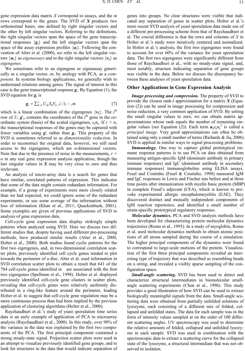

X. D. CHEN ET AL. 11

gene expression data matrix X correspond to assays, and the m

rows correspond to the genes. The SVD of X produces two

orthonormal bases, one defined by right singular vectors and

the other by left singular vectors. Referring to the definitions,

the right singular vectors span the space of the gene transcrip-

tional responses {gi} and the left singular vectors span the

space of the assay expression profiles {aj}. Following the con-

vention of Alter et al. (2000), we refer to the left singular vec-

tors {uk} as eigenassays and to the right singular vectors {vk} as

eigengenes.

We sometimes refer to an eigengene or eigenassay generi-

cally as a singular vector, or, by analogy with PCA, as a com-

ponent. In systems biology applications, we generally wish to

understand relations among genes. The signal of interest in this

case is the gene transcriptional response gi. By Equation (1), the

SVD equation for gi is

1,:1, ,

ikikkk

USVim



 g (7)

which is a linear combination of the eigengenes {vk}. The ith

row of U, g'i, contains the coordinates of the ith gene in the co-

ordinate system (basis) of the scaled eigengenes, skvk. If r < n,

the transcriptional responses of the genes may be captured with

fewer variables using g'i rather than gi. This property of the

SVD is sometimes referred to as dimensionality reduction. In

order to reconstruct the original data, however, we still need

access to the eigengenes, which are n-dimensional vectors.

Note that due to the presence of noise in the measurements, r =

n in any real gene expression analysis application, though the

last singular values in S may be very close to zero and thus

irrelevant.

An analysis of micro-array data is a search for genes that

have similar, correlated patterns of expression. This indicates

that some of the data might contain redundant information. For

example, if a group of experiments were more closely related

than we had expected, we could ignore some of the redundant

experiments, or use some average of the information without

loss of information (Khan et al., 2011; Quackenbush, 2001).

Some examples are given of previous applications of SVD to

analysis of gene expression data.

Cell-cycle gene expression data display strikingly simple

patterns when analyzed using SVD. Here we discuss two dif-

ferent studies that, despite having used different pre-processing

methods, have produced similar results (Alter et al., 2000;

Holter et al., 2000). Both studies found cyclic patterns for the

first two eigengenes, and, in two-dimensional correlation scat-

ter plots, previously identified cell cycle genes tended to plot

towards the perimeter of a disc. Alter et al. used information in

SVD correlation scatter plots to obtain a result that 641 of the

784 cell-cycle genes identified in are associated with the first

two eigengenes (Spellman et al., 1998). Holter et al. displayed

previously identified cell-cycle gene clusters in scatter plots,

revealing that cell-cycle genes were relatively uniformly dis-

tributed in a ring-like feature around the perimeter, leading

Holter et al. to suggest that cell-cycle gene regulation may be a

more continuous process than had been implied by the previous

application of clustering algorithms (Holter et al., 2000).

Raychaudhuri et al.’s study of yeast sporulation time series

data is an early example of application of PCA to microarray

analysis (Raychaudhuri et al., 2000). In this study, over 90% of

the variance in the data was explained by the first two compo-

nents of the PCA. The first principal component contained a

strong steady-state signal. Projection scatter plots were used in

an attempt to visualize previously identified gene groups, and to

look for structures in the data that would indicate separation of

genes into groups. No clear structures were visible that indi-

cated any separation of genes in scatter plots. Holter et al.’s

more recent SVD analysis of yeast sporulation data made use of

a different pre-processing scheme from that of Raychaudhuri et

al. The crucial difference is that the rows and columns of X in

Holter et al.’s study were iteratively centered and normalized.

In Holter et al.’s analysis, the first two eigengenes were found

to account for over 60% of the variance for yeast sporulation

data. The first two eigengenes were significantly different from

those of Raychaudhuri et al., with no steady-state signal, and,

most notably, structure indicating separation of gene groups

was visible in the data. Below we discuss the discrepancy be-

tween these analyses of yeast sporulation data.

Other Applications in Gene Expression Analysis

Imag e processin g an d com p ression. The property of SVD to

provide the closest rank-l approximation for a matrix X (Equa-

tion (2)) can be used in image processing for compression and

noise reduction, a very common application of SVD. By setting

the small singular values to zero, we can obtain matrix ap-

proximations whose rank equals the number of remaining sin-

gular values (see Equation (2)). Each term ukskvkT is called a

principal image. Very good approximations can often be ob-

tained using only a small number of terms (Richards & Jia, 2006).

SVD is applied in similar ways to signal processing problems.

Immunology. One way to capture global prototypical im-

mune response patterns is to use PCA on data obtained from

measuring antigen-specific IgM (dominant antibody in primary

immune responses) and IgC (dominant antibody in secondary

immune responses) immunoglobulins using ELISA assays.

Fesel and Coutinho (Fesel & Coutinho, 1998) measured IgM

and IgC responses in Lewis and Fischer rats before and at three

time points after immunization with myelin basic protein (MBP)

in complete Freud’s adjuvant (CFA), which is known to pro-

voke experimental allergic encephalomeyelitis (EAE). They

discovered distinct and mutually independent components of

IgM reaction repertoires, and identified a small number of

strain-specific prototypical regulatory responses.

Molecular dynamics. PCA and SVD analysis methods have

been developed for characterizing protein molecular dynamics

trajectories (Romo et al., 1995). In a study of myoglobin, Romo

et al. used molecular dynamics methods to obtain atomic posi-

tions of all atoms sampled during the course of a simulation.

The higher principal components of the dynamics were found

to correspond to large-scale motions of the protein. Visualiza-

tion of the first three principal components revealed an inter-

esting type of trajectory that was described as resembling beads

on a string, and revealed a visibly sparse sampling of the con-

figuration space.

Small-angle scattering. SVD has been used to detect and

characterize structural intermediates in biomolecular small-

angle scattering experiments (Chen et al., 1996). This study

provides a good illustration of how SVD can be used to extract

biologically meaningful signals from the data. Small-angle sca-

ttering data were obtained from partially unfolded solutions of

lysozyme, each consisting of a different mix of folded, col-

lapsed and unfolded states. The data for each sample was in the

form of intensity values sampled at on the order of 100 differ-

ent scattering angles. UV spectroscopy was used to determine

the relative amounts of folded, collapsed and unfolded lysozy-

me in each sample. SVD was used in combination with the

spectroscopic data to extract a scattering curve for the collapsed

state of the lysozyme, a structural intermediate that was not ob-

served in isolation.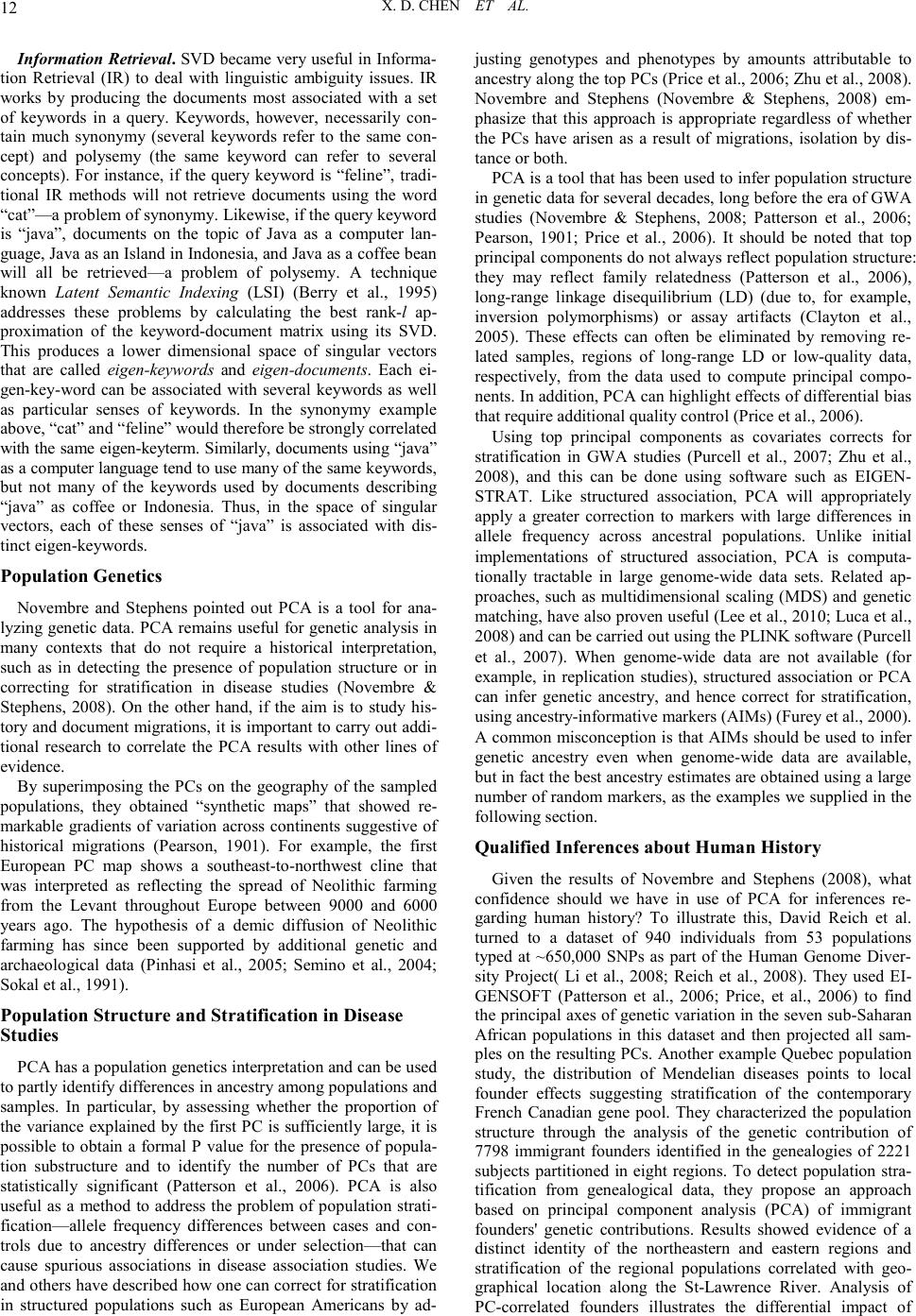

X. D. CHEN ET AL.

Information Retrieval. SVD became very useful in Informa-

tion Retrieval (IR) to deal with linguistic ambiguity issues. IR

works by producing the documents most associated with a set

of keywords in a query. Keywords, however, necessarily con-

tain much synonymy (several keywords refer to the same con-

cept) and polysemy (the same keyword can refer to several

concepts). For instance, if the query keyword is “feline”, tradi-

tional IR methods will not retrieve documents using the word

“cat”—a problem of synonymy. Likewise, if the query keyword

is “java”, documents on the topic of Java as a computer lan-

guage, Java as an Island in Indonesia, and Java as a coffee bean

will all be retrieved—a problem of polysemy. A technique

known Latent Semantic Indexing (LSI) (Berry et al., 1995)

addresses these problems by calculating the best rank-l ap-

proximation of the keyword-document matrix using its SVD.

This produces a lower dimensional space of singular vectors

that are called eigen-keywords and eigen-documents. Each ei-

gen-key-word can be associated with several keywords as well

as particular senses of keywords. In the synonymy example

above, “cat” and “feline” would therefore be strongly correlated

with the same eigen-keyterm. Similarly, documents using “java”

as a computer language tend to use many of the same keywords,

but not many of the keywords used by documents describing

“java” as coffee or Indonesia. Thus, in the space of singular

vectors, each of these senses of “java” is associated with dis-

tinct eigen-keywords.

Population Genetics

Novembre and Stephens pointed out PCA is a tool for ana-

lyzing genetic data. PCA remains useful for genetic analysis in

many contexts that do not require a historical interpretation,

such as in detecting the presence of population structure or in

correcting for stratification in disease studies (Novembre &

Stephens, 2008). On the other hand, if the aim is to study his-

tory and document migrations, it is important to carry out addi-

tional research to correlate the PCA results with other lines of

evidence.

By superimposing the PCs on the geography of the sampled

populations, they obtained “synthetic maps” that showed re-

markable gradients of variation across continents suggestive of

historical migrations (Pearson, 1901). For example, the first

European PC map shows a southeast-to-northwest cline that

was interpreted as reflecting the spread of Neolithic farming

from the Levant throughout Europe between 9000 and 6000

years ago. The hypothesis of a demic diffusion of Neolithic

farming has since been supported by additional genetic and

archaeological data (Pinhasi et al., 2005; Semino et al., 2004;

Sokal et al., 1991).

Population Structure and Stratification in Disease

Studies

PCA has a population genetics interpretation and can be used

to partly identify differences in ancestry among populations and

samples. In particular, by assessing whether the proportion of

the variance explained by the first PC is sufficiently large, it is

possible to obtain a formal P value for the presence of popula-

tion substructure and to identify the number of PCs that are

statistically significant (Patterson et al., 2006). PCA is also

useful as a method to address the problem of population strati-

fication—allele frequency differences between cases and con-

trols due to ancestry differences or under selection—that can

cause spurious associations in disease association studies. We

and others have described how one can correct for stratification

in structured populations such as European Americans by ad-

justing genotypes and phenotypes by amounts attributable to

ancestry along the top PCs (Price et al., 2006; Zhu et al., 2008).

Novembre and Stephens (Novembre & Stephens, 2008) em-

phasize that this approach is appropriate regardless of whether

the PCs have arisen as a result of migrations, isolation by dis-

tance or both.

PCA is a tool that has been used to infer population structure

in genetic data for several decades, long before the era of GWA

studies (Novembre & Stephens, 2008; Patterson et al., 2006;

Pearson, 1901; Price et al., 2006). It should be noted that top

principal components do not always reflect population structure:

they may reflect family relatedness (Patterson et al., 2006),

long-range linkage disequilibrium (LD) (due to, for example,

inversion polymorphisms) or assay artifacts (Clayton et al.,

2005). These effects can often be eliminated by removing re-

lated samples, regions of long-range LD or low-quality data,

respectively, from the data used to compute principal compo-

nents. In addition, PCA can highlight effects of differential bias

that require additional quality control (Price et al., 2006).

Using top principal components as covariates corrects for

stratification in GWA studies (Purcell et al., 2007; Zhu et al.,

2008), and this can be done using software such as EIGEN-

STRAT. Like structured association, PCA will appropriately

apply a greater correction to markers with large differences in

allele frequency across ancestral populations. Unlike initial

implementations of structured association, PCA is computa-

tionally tractable in large genome-wide data sets. Related ap-

proaches, such as multidimensional scaling (MDS) and genetic

matching, have also proven useful (Lee et al., 2010; Luca et al.,

2008) and can be carried out using the PLINK software (Purcell

et al., 2007). When genome-wide data are not available (for

example, in replication studies), structured association or PCA

can infer genetic ancestry, and hence correct for stratification,

using ancestry-informative markers (AIMs) (Furey et al., 2000).

A common misconception is that AIMs should be used to infer

genetic ancestry even when genome-wide data are available,

but in fact the best ancestry estimates are obtained using a large

number of random markers, as the examples we supplied in the

following section.

Qualified Inferences about Human History

Given the results of Novembre and Stephens (2008), what

confidence should we have in use of PCA for inferences re-

garding human history? To illustrate this, David Reich et al.

turned to a dataset of 940 individuals from 53 populations

typed at ~650,000 SNPs as part of the Human Genome Diver-

sity Project( Li et al., 2008; Reich et al., 2008). They used EI-

GENSOFT (Patterson et al., 2006; Price, et al., 2006) to find

the principal axes of genetic variation in the seven sub-Saharan

African populations in this dataset and then projected all sam-

ples on the resulting PCs. Another example Quebec population

study, the distribution of Mendelian diseases points to local

founder effects suggesting stratification of the contemporary

French Canadian gene pool. They characterized the population

structure through the analysis of the genetic contribution of

7798 immigrant founders identified in the genealogies of 2221

subjects partitioned in eight regions. To detect population stra-

tification from genealogical data, they propose an approach

based on principal component analysis (PCA) of immigrant

founders' genetic contributions. Results showed evidence of a

distinct identity of the northeastern and eastern regions and

stratification of the regional populations correlated with geo-

graphical location along the St-Lawrence River. Analysis of

PC-correlated founders illustrates the differential impact of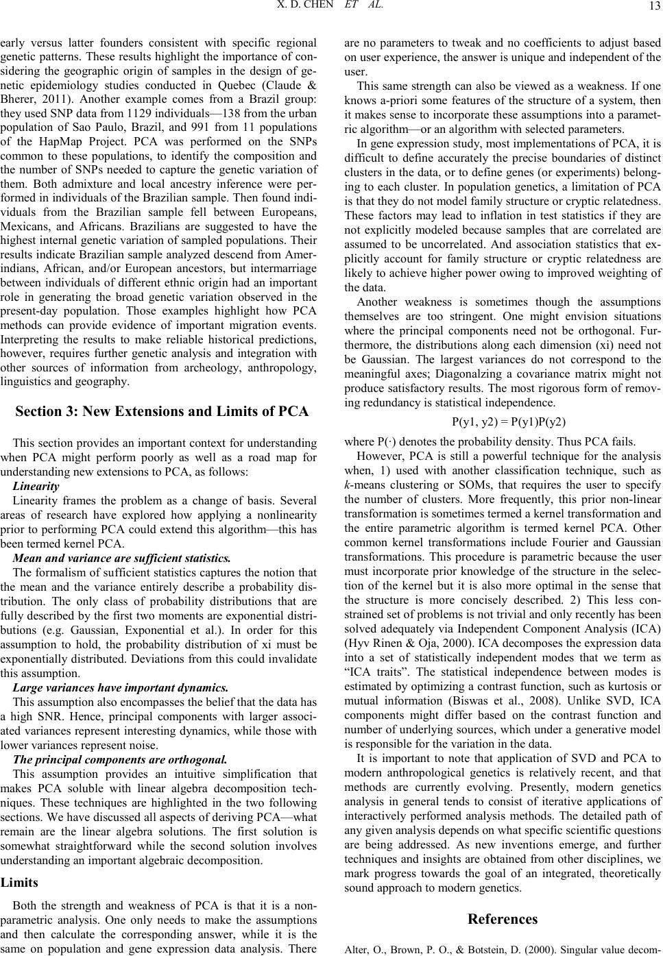

X. D. CHEN ET AL. 13

early versus latter founders consistent with specific regional

genetic patterns. These results highlight the importance of con-

sidering the geographic origin of samples in the design of ge-

netic epidemiology studies conducted in Quebec (Claude &

Bherer, 2011). Another example comes from a Brazil group:

they used SNP data from 1129 individuals—138 from the urban

population of Sao Paulo, Brazil, and 991 from 11 populations

of the HapMap Project. PCA was performed on the SNPs

common to these populations, to identify the composition and

the number of SNPs needed to capture the genetic variation of

them. Both admixture and local ancestry inference were per-

formed in individuals of the Brazilian sample. Then found indi-

viduals from the Brazilian sample fell between Europeans,

Mexicans, and Africans. Brazilians are suggested to have the

highest internal genetic variation of sampled populations. Their

results indicate Brazilian sample analyzed descend from Amer-

indians, African, and/or European ancestors, but intermarriage

between individuals of different ethnic origin had an important

role in generating the broad genetic variation observed in the

present-day population. Those examples highlight how PCA

methods can provide evidence of important migration events.

Interpreting the results to make reliable historical predictions,

however, requires further genetic analysis and integration with

other sources of information from archeology, anthropology,

linguistics and geography.

Section 3: New Extensions and Limits of PCA

This section provides an important context for understanding

when PCA might perform poorly as well as a road map for

understanding new extensions to PCA, as follows:

Linearity

Linearity frames the problem as a change of basis. Several

areas of research have explored how applying a nonlinearity

prior to performing PCA could extend this algorithm—this has

been termed kernel PCA.

Mean an d variance a r e sufficient sta tistics.

The formalism of sufficient statistics captures the notion that

the mean and the variance entirely describe a probability dis-

tribution. The only class of probability distributions that are

fully described by the first two moments are exponential distri-

butions (e.g. Gaussian, Exponential et al.). In order for this

assumption to hold, the probability distribution of xi must be

exponentially distributed. Deviations from this could invalidate

this assumption.

Large variances have important dynamics.

This assumption also encompasses the belief that the data has

a high SNR. Hence, principal components with larger associ-

ated variances represent interesting dynamics, while those with

lower variances represent noise.

The principal components are orthogonal.

This assumption provides an intuitive simplification that

makes PCA soluble with linear algebra decomposition tech-

niques. These techniques are highlighted in the two following

sections. We have discussed all aspects of deriving PCA—what

remain are the linear algebra solutions. The first solution is

somewhat straightforward while the second solution involves

understanding an important algebraic decomposition.

Limits

Both the strength and weakness of PCA is that it is a non-

parametric analysis. One only needs to make the assumptions

and then calculate the corresponding answer, while it is the

same on population and gene expression data analysis. There

are no parameters to tweak and no coefficients to adjust based

on user experience, the answer is unique and independent of the

user.

This same strength can also be viewed as a weakness. If one

knows a-priori some features of the structure of a system, then

it makes sense to incorporate these assumptions into a paramet-

ric algorithm—or an algorithm with selected parameters.

In gene expression study, most implementations of PCA, it is

difficult to define accurately the precise boundaries of distinct

clusters in the data, or to define genes (or experiments) belong-

ing to each cluster. In population genetics, a limitation of PCA

is that they do not model family structure or cryptic relatedness.

These factors may lead to inflation in test statistics if they are

not explicitly modeled because samples that are correlated are

assumed to be uncorrelated. And association statistics that ex-

plicitly account for family structure or cryptic relatedness are

likely to achieve higher power owing to improved weighting of

the data.

Another weakness is sometimes though the assumptions

themselves are too stringent. One might envision situations

where the principal components need not be orthogonal. Fur-

thermore, the distributions along each dimension (xi) need not

be Gaussian. The largest variances do not correspond to the

meaningful axes; Diagonalzing a covariance matrix might not

produce satisfactory results. The most rigorous form of remov-

ing redundancy is statistical independence.

P(y1, y2) = P(y1)P(y2)

where P(·) denotes the probability density. Thus PCA fails.

However, PCA is still a powerful technique for the analysis

when, 1) used with another classification technique, such as

k-means clustering or SOMs, that requires the user to specify

the number of clusters. More frequently, this prior non-linear

transformation is sometimes termed a kernel transformation and

the entire parametric algorithm is termed kernel PCA. Other

common kernel transformations include Fourier and Gaussian

transformations. This procedure is parametric because the user

must incorporate prior knowledge of the structure in the selec-

tion of the kernel but it is also more optimal in the sense that

the structure is more concisely described. 2) This less con-

strained set of problems is not trivial and only recently has been

solved adequately via Independent Component Analysis (ICA)

(Hyv Rinen & Oja, 2000). ICA decomposes the expression data

into a set of statistically independent modes that we term as

“ICA traits”. The statistical independence between modes is

estimated by optimizing a contrast function, such as kurtosis or

mutual information (Biswas et al., 2008). Unlike SVD, ICA

components might differ based on the contrast function and

number of underlying sources, which under a generative model

is responsible for the variation in the data.

It is important to note that application of SVD and PCA to

modern anthropological genetics is relatively recent, and that

methods are currently evolving. Presently, modern genetics

analysis in general tends to consist of iterative applications of

interactively performed analysis methods. The detailed path of

any given analysis depends on what specific scientific questions

are being addressed. As new inventions emerge, and further

techniques and insights are obtained from other disciplines, we

mark progress towards the goal of an integrated, theoretically

sound approach to modern genetics.

References

Alter, O., Brown, P. O., & Botstein, D. (2000). Singular value decom-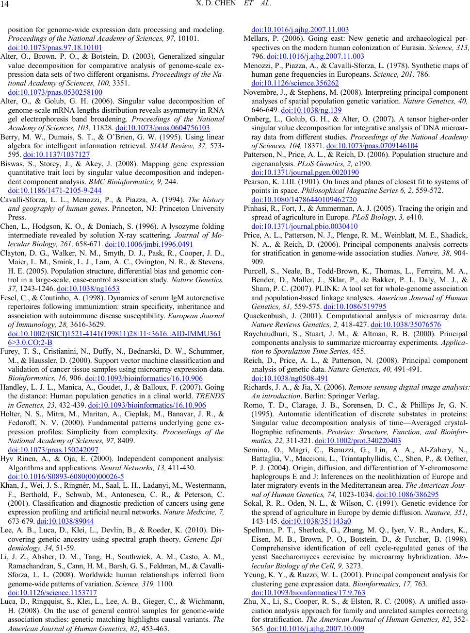

X. D. CHEN ET AL.

position for genome-wide expression data processing and modeling.

Proceedin gs of the N ation al Academ y of Scien ces, 97 , 10101.

doi:10.1073/pnas.97.18.10101

Alter, O., Brown, P. O., & Botstein, D. (2003). Generalized singular

value decomposition for comparative analysis of genome-scale ex-

pression data sets of two different organisms. Proceedings of the Na-

tional Academy of Sciences, 100, 3351.

doi:10.1073/pnas.0530258100

Alter, O., & Golub, G. H. (2006). Singular value decomposition of

genome-scale mRNA lengths distribution reveals asymmetry in RNA

gel electrophoresis band broadening. Proceedings of the National

Academy of Sciences, 103, 11828. doi:10.1073/pnas.0604756103

Berry, M. W., Dumais, S. T., & O’Brien, G. W. (1995). Using linear

algebra for intelligent information retrieval. SIAM Review, 37, 573-

595. doi:10.1137/1037127

Biswas, S., Storey, J., & Akey, J. (2008). Mapping gene expression

quantitative trait loci by singular value decomposition and indepen-

dent component analysis. BMC Bioinformatics, 9, 244.

doi:10.1186/1471-2105-9-244

Cavalli-Sforza, L. L., Menozzi, P., & Piazza, A. (1994). The history

and geography of human genes. Princeton, NJ: Princeton University

Press.

Chen, L., Hodgson, K. O., & Doniach, S. (1996). A lysozyme folding

intermediate revealed by solution X-ray scattering. Journal of Mo-

lecular Biology, 261, 658-671. doi:10.1006/jmbi.1996.0491

Clayton, D. G., Walker, N. M., Smyth, D. J., Pask, R., Cooper, J. D.,

Maier, L. M., Smink, L. J., Lam, A. C., Ovington, N. R., & Stevens,

H. E. (2005). Population structure, differential bias and genomic con-

trol in a large-scale, case-control association study. Natu re Genet ics,

37, 1243-1246. doi:10.1038/ng1653

Fesel, C., & Coutinho, A. (1998). Dynamics of serum IgM autoreactive

repertoires following immunization: strain specificity, inheritance and

association with autoimmune disease susceptibility. European Journal

of Immunology, 28, 3616-3629.

doi:10.1002/(SICI)1521-4141(199811)28:11<3616::AID-IMMU361

6>3.0.CO;2-B

Furey, T. S., Cristianini, N., Duffy, N., Bednarski, D. W., Schummer,

M., & Haussler, D. (2000). Support vector machine classification and

validation of cancer tissue samples using microarray expression data.

Bioi nf or m a ti cs , 1 6, 906. doi:10.1093/bioinformatics/16.10.906

Handley, L. J. L., Manica, A., Goudet, J., & Balloux, F. (2007). Going

the distance: Human population genetics in a clinal world. TRENDS

in Genetics, 23, 432-439. doi:10.1093/bioinformatics/16.10.906

Holter, N. S., Mitra, M., Maritan, A., Cieplak, M., Banavar, J. R., &

Fedoroff, N. V. (2000). Fundamental patterns underlying gene ex-

pression profiles: Simplicity from complexity. Proceedings of the

National Academy of Sciences, 97, 8409.

doi:10.1073/pnas.150242097

Hyv Rinen, A., & Oja, E. (2000). Independent component analysis:

Algorithms and applications. Neura l Networ ks , 13, 411-430.

doi:10.1016/S0893-6080(00)00026-5

Khan, J., Wei, J. S., Ringnér, M., Saal, L. H., Ladanyi, M., Westermann,

F., Berthold, F., Schwab, M., Antonescu, C. R., & Peterson, C.

(2001). Classification and diagnostic prediction of cancers using gene

expression profiling and artificial neural networks. Natu re Me dic i ne , 7,

673-679. doi:10.1038/89044

Lee, A. B., Luca, D., Klei, L., Devlin, B., & Roeder, K. (2010). Dis-

covering genetic ancestry using spectral graph theory. Genetic Epi-

demiology, 34, 51-59.

Li, J. Z., Absher, D. M., Tang, H., Southwick, A. M., Casto, A. M.,

Ramachandran, S., Cann, H. M., Barsh, G. S., Feldman, M., & Cavalli-

Sforza, L. L. (2008). Worldwide human relationships inferred from

genome-wide patterns of variation. Sci ence, 319, 1100.

doi:10.1126/science.1153717

Luca, D., Ringquist, S., Klei, L., Lee, A. B., Gieger, C., & Wichmann,

H. (2008). On the use of general control samples for genome-wide

association studies: genetic matching highlights causal variants. The

American Journal of Huma n Geneti cs, 82, 453-463.

doi:10.1016/j. aj h g.20 07 .11.003

Mellars, P. (2006). Going east: New genetic and archaeological per-

spectives on the modern human colonization of Eurasia. Sc ienc e , 313,

796. doi:10.1016/j.ajhg.2007.11.003

Menozzi, P., Piazza, A., & Cavalli-Sforza, L. (1978). Synthetic maps of

human gene frequencies in Europeans. Scienc e, 201, 786.

doi:10.1126/sc i en c e.35 626 2

Novembre, J., & Stephens, M. (2008). Interpreting principal component

analyses of spatial population genetic variation. Nature Genetics, 40,

646-649. doi:10.1038/ng.139

Omberg, L., Golub, G. H., & Alter, O. (2007). A tensor higher-order

singular value decomposition for integrative analysis of DNA microar-

ray data from different studies. Proceedings of the National Academy

of Sciences , 104, 18371. doi:10.1073/pnas.0709146104

Patterson, N., Price, A. L., & Reich, D. (2006). Population structure and

eigenanalysis. PLoS Gene tics, 2, e190.

doi:10.1371/journal.pgen.0020190

Pearson, K. LIII. (1901). On lines and planes of closest fit to systems of

points in space. Ph il osop hi c al Magaz i ne Se r ies 6, 2, 559-572.

doi:10.1080/14786440109462720

Pinhasi, R., Fort, J., & Ammerman, A. J. (2005). Tracing the origin and

spread of agriculture in Europe. PLoS Biology, 3, e410.

doi:10.1371/journal.pbio.0030410

Price, A. L., Patterson, N. J., Plenge, R. M., Weinblatt, M. E., Shadick,

N. A., & Reich, D. (2006). Principal components analysis corrects

for stratification in genome-wide association studies. Nature, 38, 904-

909.

Purcell, S., Neale, B., Todd-Brown, K., Thomas, L., Ferreira, M. A.,

Bender, D., Maller, J., Sklar, P., de Bakker, P. I., Daly, M. J., &

Sham, P. C. (2007). PLINK: A tool set for whole-genome association

and population-based linkage analyses. American Journal of Human

Genetics, 81, 559-575. doi:10.1086/519795

Quackenbush, J. (2001). Computational analysis of microarray data.

Nature Re view s Geneti cs, 2, 418 -427. doi:10.1038/35076576

Raychaudhuri, S., Stuart, J. M., & Altman, R. B. (2000). Principal

components analysis to summarize microarray experiments. Appl ica -

tion to Sporulation Time Series, 455.

Reich, D., Price, A. L., & Patterson, N. (2008). Principal component

analysis of genetic data. Nature Genetics, 40 , 491-491.

doi:10.1038/ng0508-491

Richards, J. A., & Jia, X. (2006). Remote sensing digital image analysis:

An intr od uctio n. Berlin: Springer Verlag.

Romo, T. D., Clarage, J. B., Sorensen, D. C., & Phillips Jr, G. N.

(1995). Automatic identification of discrete substates in proteins:

Singular value decomposition analysis of time—Averaged crystal-

llographic refinements. Proteins: Structure, Function, and Bioinfor-

matics, 22, 311-321. doi:10.1002/prot.340220403

Semino, O., Magri, C., Benuzzi, G., Lin, A. A., Al-Zahery, N.,

Battaglia, V., Maccioni, L., Triantaphyllidis, C., Shen, P., & Oefner,

P. J. (2004). Origin, diffusion, and differentiation of Y-chromosome

haplogroups E and J: Inferences on the neolithization of Europe and

later migratory events in the Mediterranean area. The American Jour-

nal of Human Genetics, 74, 1023-1034. doi:10.1086/386295

Sokal, R. R., Oden, N. L., & Wilson, C. (1991). Genetic evidence for

the spread of agriculture in Europe by demic diffusion. Nauture, 351,

143-145. doi:10.1038/351143a0

Spellman, P. T., Sherlock, G., Zhang, M. Q., Iyer, V. R., Anders, K.,

Eisen, M. B., Brown, P. O., Botstein, D., & Futcher, B. (1998).

Comprehensive identification of cell cycle-regulated genes of the

yeast Saccharomyces cerevisiae by microarray hybridization. Mo-

lecular Biology of the Cell, 9, 3273.

Yeung, K. Y., & Ruzzo, W. L. (2001). Principal component analysis for

clustering gene expression data. Bioinfo r matics, 17, 763.

doi:10.1093/bioinformatics/17.9.763

Zhu, X., Li, S., Cooper, R. S., & Elston, R. C. (2008). A unified asso-

ciation analysis approach for family and unrelated samples correcting

for stratification. The America n Jou rna l of Hu man Gen et ics , 82 , 352-

365. doi:10.1016/j.ajhg.2007.10.009