

Paper Menu >>
Journal Menu >>
 Journal of Mathematical Finance, 2011, 1, 58-62 doi:10.4236/jmf.2011.13008 Published Online November 2011 (http://www.SciRP.org/journal/jmf) Copyright © 2011 SciRes. JMF Maximum Quasi-Likelihood Estimation in Fractional Levy Stochastic Volatility Model Jaya Prakasah Narayan Bishwal Department of Mathematics and Statistics, University of North Carolina at Charlotte, Charlotte, USA E-mail: [email protected] Received July 13, 2011; revised August 12, 2011; accepted August 22, 2011 Abstract Usually asset price process has jumps and volatility process has long memory. We study maximum quasi- likelihood estimators for the parameters of a fractionally integrated exponential GARCH, in short FIECO- GARCH process based on discrete observations. We deal with a compound Poisson FIECOGARCH process and study the asymptotic behavior of the maximum quasi-likelihood estimator. We show that the resulting estimators are consistent and asymptotically normal. Keywords: Stochastic Volatility, Long Memory Process, Jump Process, Fractional Levy Process, Poisson Process, Ornstein-Uhlenbeck Process, Gaussian Quasi-Likelihood, Consistency, Asymptotic Normality 1. Introduction Parameter estimation in GARCH models has been studi- ed extensively in view of their wide applications. In or- der to incorporate long memory in the model we look at the continuous time counterpart. Most of the financial transactions are recorded these days with ultra high fre- quency which are also called tick-by-tick data. The most important feature of these data are irregular spacing of observation time points. If one aggregates the data up to fixed time intervals, there is loss of information which should be avoided. Hence it is natural to model price processes in continuous time. Also volatility clusters on high level. This long-run volatility persistence is not taken into account by GARCH models. Levy processes con- tribute non-normality and jumps in the observed part of the model and fractional processes contribute long me- mory in unobserved part in the model. Based on discrete observations of the price process we estimate all the un- known parameters of the price and the volatility process by the maximum quasi-likelihood estimation. We use Gaussian quasi-likelihood as a contrast function. Maxi- mum quasi-likelihood estimator is an application of Kal- man filter in the context of maximum likelihood estima- tion. Even if the data are non-normal, we use the Gaus- sian log-likelihood. Non-negative Ornstein-Uhlenbeck processes were first studied by Wolfe [1] who obtained it as a limit of an au- toregressive process with positive innovations. These days non-negative Ornstein-Uhlenbeck processes have recei- ved lot of attention in view of their applications as inter- est rate and stochastic volatility models, see Barndorff- Nielsen and Shephard [2,3]. Gaver and Lewis [4] studied estimation in first order autoregressive gamma process. Davis and McCormick [5] studied estimation for first or- der autoregressive process with positive or bounded in- novations. Neilsen and Shephard [6] studied likelihood analysis of a first order autoregressive model with expo- nential innovations. Brockwell, Davis and Yang [7] stu- died parameter estimation of non-negative Levy driven Ornstein-Uhlenbeck processes. Jongbloed, van der Meulen and van der Vaart [8] studied nonparametric estimation for Levy driven Ornstein-Uhlenbeck processes. Parameter estimation in Gaussian Ornstein-Uhlenbeck process was extensively studied in Bishwal [9]. To ac- count for the strong persistence in volatility, which sometimes is observed in empirical data, we study the FIECOGARCH (fractionally integrated exponential con- tinuous time generalized autoregressive conditional het- eroscedastic) process. The log-price process has jumps and the log-volatility process has long memory. The long memory effect introduced in the log-volatility process, propagates to the volatility process. Thus the model here captures the two stylized facts of long memory and jumps. Continuous time long memory process in volatility re- ceived some attention, see Comte and Renault [10] where they used fractional Ornstein-Uhlenbeck process as the stochastic volatility process and Comte, Coutin and Renault 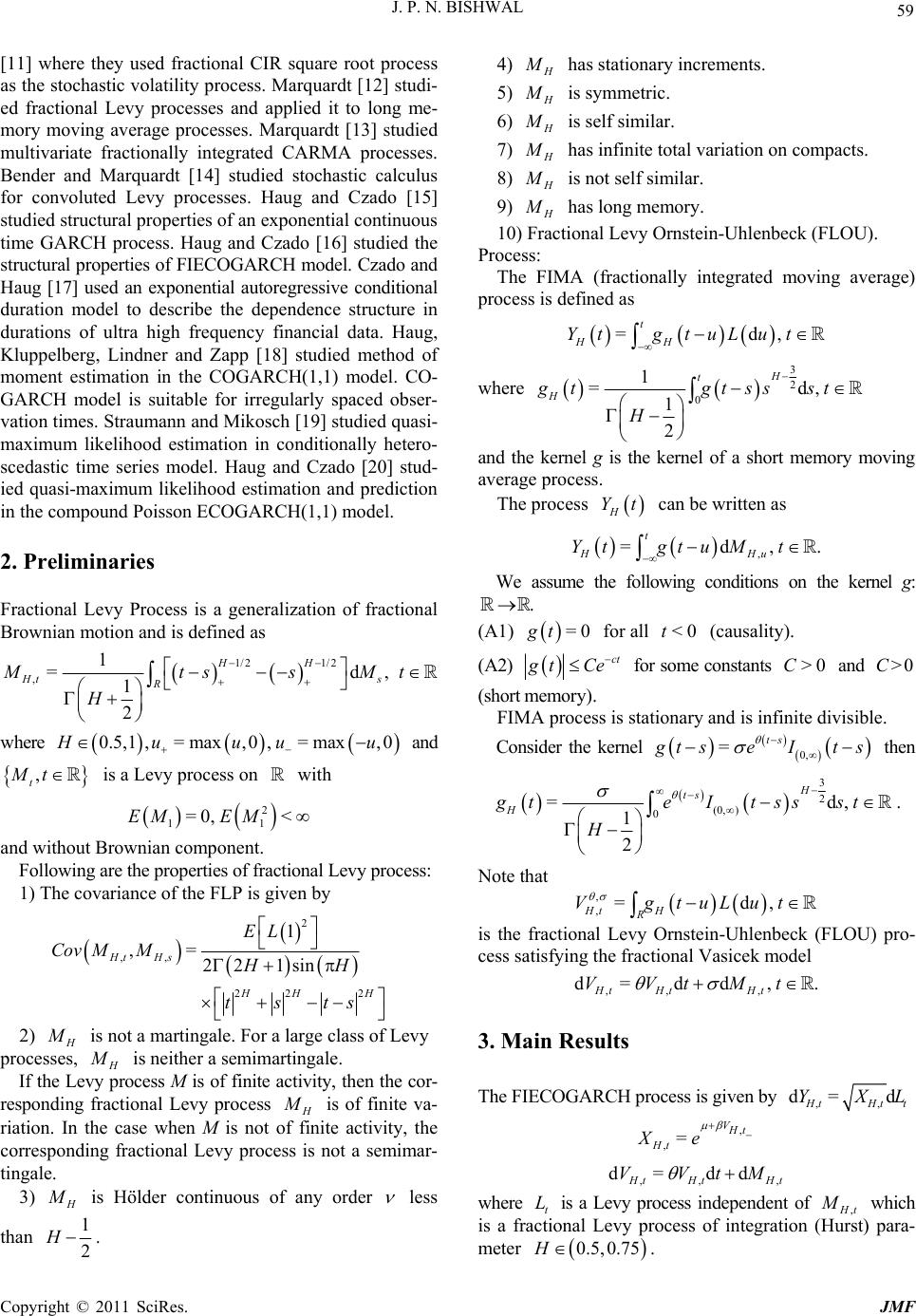 59 J. P. N. BISHWAL [11] where they used fractional CIR square root process as the stochastic volatility process. Marquardt [12] studi- ed fractional Levy processes and applied it to long me- mory moving average processes. Marquardt [13] studied multivariate fractionally integrated CARMA processes. Bender and Marquardt [14] studied stochastic calculus for convoluted Levy processes. Haug and Czado [15] studied structural properties of an exponential continuous time GARCH process. Haug and Czado [16] studied the structural properties of FIECOGARCH model. Czado and Haug [17] used an exponential autoregressive conditional duration model to describe the dependence structure in durations of ultra high frequency financial data. Haug, Kluppelberg, Lindner and Zapp [18] studied method of moment estimation in the COGARCH(1,1) model. CO- GARCH model is suitable for irregularly spaced obser- vation times. Straumann and Mikosch [19] studied quasi- maximum likelihood estimation in conditionally hetero- scedastic time series model. Haug and Czado [20] stud- ied quasi-maximum likelihood estimation and prediction in the compound Poisson ECOGARCH(1,1) model. 2. Preliminaries Fractional Levy Process is a generalization of fractional Brownian motion and is defined as 1/21/2 , 1 =d 1 2 HH Ht s R MtssMt H , where 0.5,1,= max,0,= max,0 H uuu u and is a Levy process on with , t Mt 2 11 =0, <EMEM and without Brownian component. Following are the properties of fractional Levy process: 1) The covariance of the FLP is given by 2 ,, 22 2 1 ,= 22 1sin Ht Hs HH H EL Cov MMHH tsts 2) H M is not a martingale. For a large class of Levy processes, H M is neither a semimartingale. If the Levy process M is of finite activity, then the cor- responding fractional Levy process H M is of finite va- riation. In the case when M is not of finite activity, the corresponding fractional Levy process is not a semimar- tingale. 3) H M is Hölder continuous of any order less than 1 2 H. 4) H M has stationary increments. 5) H M is symmetric. 6) H M is self similar. 7) H M has infinite total variation on compacts. 8) H M is not self similar. 9) H M has long memory. 10) Fractional Levy Ornstein-Uhlenbeck (FLOU). Process: The FIMA (fractionally integrated moving average) process is defined as =d t HH Yt gtuLut, where 3 2 0 1 =d 1 2 H t H gtgtss st H , and the kernel g is the kernel of a short memory moving average process. The process H Yt can be written as , =d, . t HH YtgtuMt u We assume the following conditions on the kernel g: . (A1) =0gt for all (causality). <0t (A2) ct g tCe for some constants and (short memory). >0C>0C FIMA process is stationary and is infinite divisible. Consider the kernel 0, =ts g tse Its then 3 2 (0, ) 0 =d 1 2 H ts H gte Itssst H , . Note that , ,=d , Ht H R VgtuLut is the fractional Levy Ornstein-Uhlenbeck (FLOU) pro- cess satisfying the fractional Vasicek model ,, , d=dd, . Ht HtHt VVtMt 3. Main Results The FIECOGARCH process is given by ,, d= d H tHt YX t L , ,=V H t Ht Xe ,, d= dd , H tHtH VVtM t where t is a Levy process independent of , L H t which is a fractional Levy process of integration (Hurst) para- meter M 0.5,0.75H. Copyright © 2011 SciRes. JMF 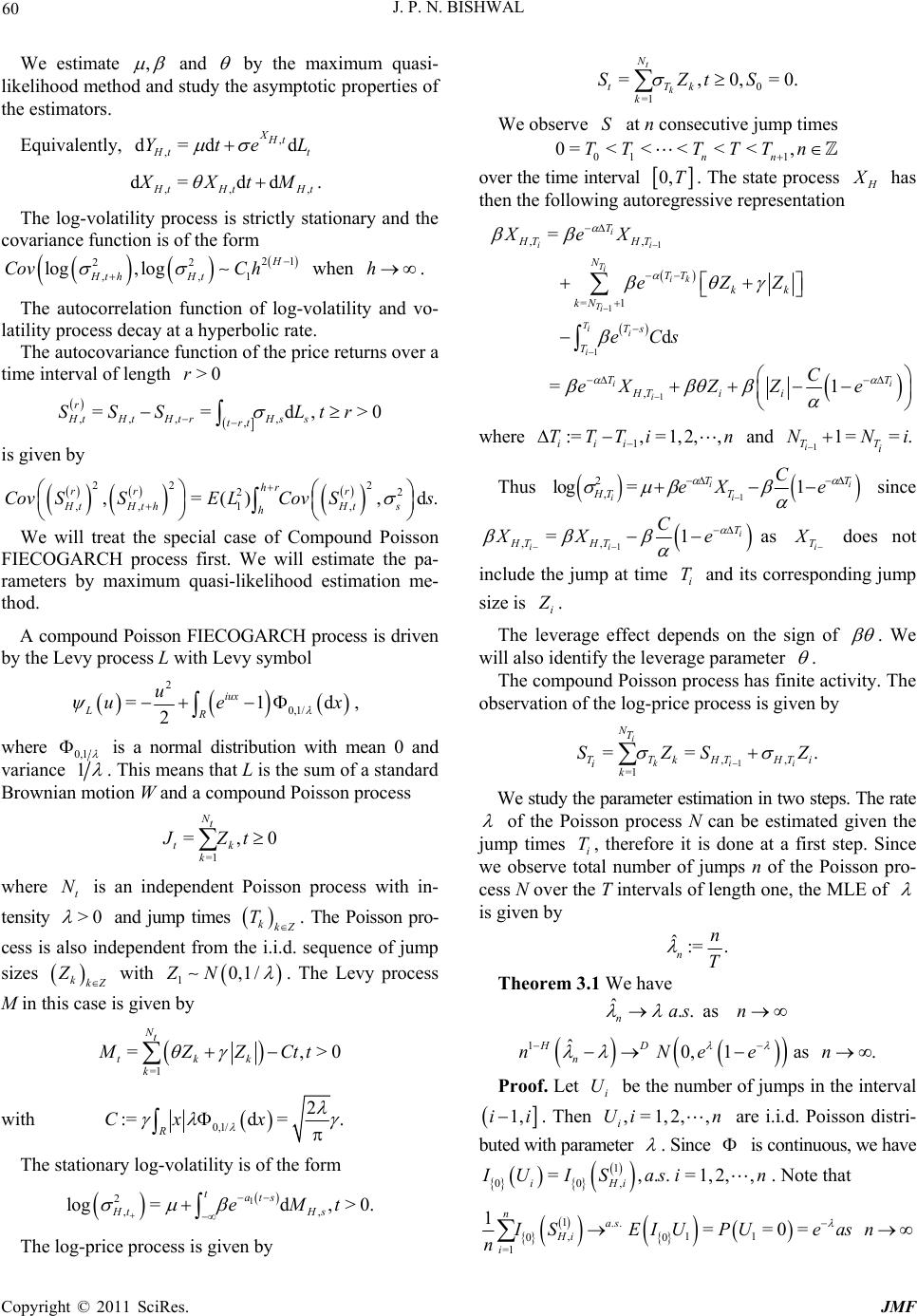 60 J. P. N. BISHWAL We estimate , and by the maximum quasi- likelihood method and study the asymptotic properties of the estimators. Equivalently, , , d=dd XHt H tt Yte L , ,, d= dd H tHt XXtM Ht . The log-volatility process is strictly stationary and the covariance function is of the form when . 21 22 ,,1 log, log H Ht hHt CovC hh The autocorrelation function of log-volatility and vo- latility process decay at a hyperbolic rate. The autocovariance function of the price returns over a time interval of length >0r ,,, , , ==d, r HtHtHt rHss trt SSS Ltr >0 d. is given by 22 2 22 ,, 1, ,=() , hr rr r HtHt hHts h Cov SSELCov Ss We will treat the special case of Compound Poisson FIECOGARCH process first. We will estimate the pa- rameters by maximum quasi-likelihood estimation me- thod. A compound Poisson FIECOGARCH process is driven by the Levy process L with Levy symbol 2 0,1/ =1 2 iux LR u ue d x , where 0,1 is a normal distribution with mean 0 and variance 1 . This means that L is the sum of a standard Brownian motion W and a compound Poisson process =1 =, Nt tk k JZt 0 where is an independent Poisson process with in- tensity t N >0 and jump times kkZ T 0,1/ . The Poisson pro- cess is also independent from the i.i.d. sequence of jump sizes with ZN k ZkZ 1 . The Levy process M in this case is given by =1 =, Nt tkk k MZZCtt >0 with 0,1/ 2 :=d =. R Cx x The stationary log-volatility is of the form 1 2 ,, log=d,> 0. tats Ht Hs eMt The log-price process is given by 0 =1 =,0, t k N tTk k SZtS=0. We observe at n consecutive jump times S 01 1 0=<<<< <, nn TTTTTn over the time interval 0,T. The state process H X has then the following autoregressive representation 1 1 1 1 ,, =1 , = d =1 i ii Ti ik Ti Tii i ii i T HT HT N TT kk kN Ts T TT HTi i XeX eZZ eCs C eXZ Ze where 1 :=,= 1, 2,, iii TTTin and 11== . i TT i NN i Thus 1 2 , log =1 ii ii TT HT T C eX e since 1 ,, =1 i ii T HT HT C XX e as i T X does not include the jump at time and its corresponding jump size is i T i Z . The leverage effect depends on the sign of . We will also identify the leverage parameter . The compound Poisson process has finite activity. The observation of the log-price process is given by 1 ,, =1 == i ki NT TTkHTHT ik SZS . i i Z We study the parameter estimation in two steps. The rate of the Poisson process N can be estimated given the jump times i, therefore it is done at a first step. Since we observe total number of jumps n of the Poisson pro- cess N over the T intervals of length one, the MLE of T is given by ˆ:= . n n T Theorem 3.1 We have ˆ .. as nasn 1ˆ0,1 as. HD n nNee U n Proof. Let be the number of jumps in the interval i 1,ii. Then are i.i.d. Poisson distri- buted with parameter ,=1,2, ,Uin i . Since is continuous, we have , =,.. = i 1 iH 00 ,2,1, I UISasi n. Note that 1.. ,11 00 =1 1==0= nas Hi i ISEIU PUeasn n C opyright © 2011 SciRes. JMF 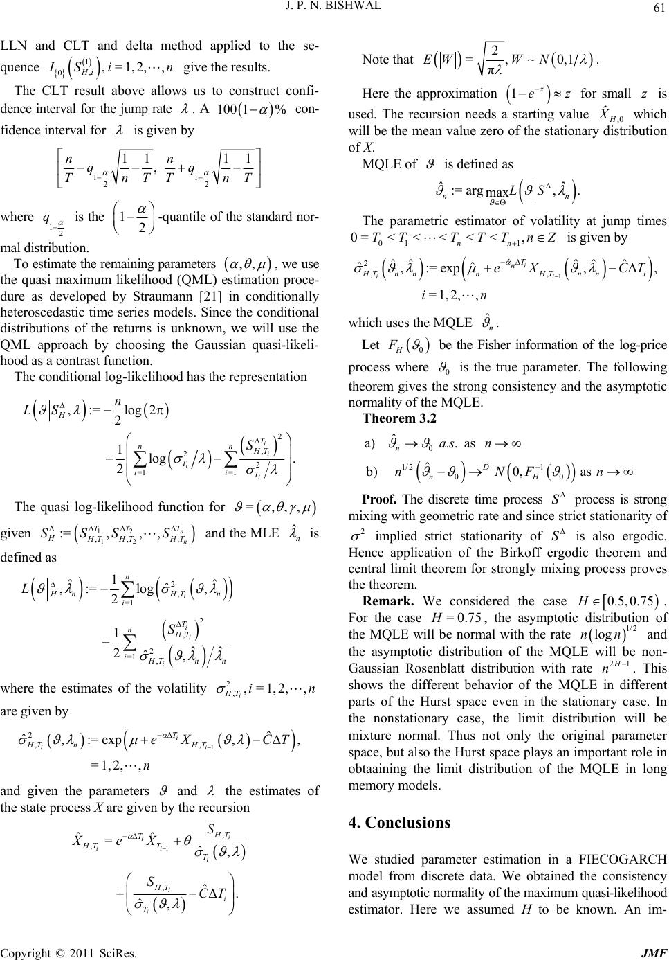 61 J. P. N. BISHWAL LLN and CLT and delta method applied to the se- quence 1 , 0,= 1, 2,, Hi I Si n give the results. The CLT result above allows us to construct confi- dence interval for the jump rate . A 100 1% con- fidence interval for is given by 11 22 11 11 , nn qq TnTTn T where 12 q is the 12 -quantile of the standard nor- mal distribution. To estimate the remaining parameters ,, , we use the quasi maximum likelihood (QML) estimation proce- dure as developed by Straumann [21] in conditionally heteroscedastic time series models. Since the conditional distributions of the returns is unknown, we will use the QML approach by choosing the Gaussian quasi-likeli- hood as a contrast function. The conditional log-likelihood has the representation 2 , 2 2 =1 =1 ,:= log2 2 1log . 2 i i i i H T nn HT T ii T n LS S The quasi log-likelihood function for =,,, ˆn given and the MLE 12 12 ,,, :=,,, n n T TT HHT HTHT SSS S is defined as 2 , =1 2 , 2 =1 , 1 ˆ ˆ ,:= log, 2 1 ˆˆ 2ˆ, i i i i n HnHTn i T nHT i ˆ H Tn L S n where the estimates of the volatility are given by 2 ,,= 1, 2,, i HT in , 1 2 ,, ˆ ˆ,:=exp , =1,2, , i ii T HT nHT eX CT n and given the parameters and the estimates of the state process X are given by the recursion 1 , , , ˆˆ =ˆ, ˆ. ˆ, i i ii i i i i HT T HT T T HT T S XeX SCT Note that 2 =, 0,1 π EWW N. Here the approximation for small is 1z e zz used. The recursion needs a starting value ,0 ˆ H X which will be the mean value zero of the stationary distribution of X. MQLE of is defined as ˆˆ := arg,. max nn LS The parametric estimator of volatility at jump times is given by 01 1 0=<<<< <, nn TT TTTnZ 1 ˆ 2 ,, ˆˆˆˆˆ ˆˆ ,:=exp, , =1,2, , i ii T n HTn nnHTn ni eX CT in which uses the MQLE ˆn . Let 0H F be the Fisher information of the log-price process where 0 is the true parameter. The following theorem gives the strong consistency and the asymptotic normality of the MQLE. Theorem 3.2 0 ˆ a).. as nasn 1/21 00 ˆ b)0, as D nH nNFn Proof. The discrete time process process is strong mixing with geometric rate and since strict stationarity of S 2 implied strict stationarity of is also ergodic. Hence application of the Birkoff ergodic theorem and central limit theorem for strongly mixing process proves the theorem. S Remark. We considered the case 0.5,0.75H 1/2 lognn 21H n . For the case , the asymptotic distribution of the MQLE will be normal with the rate and the asymptotic distribution of the MQLE will be non- Gaussian Rosenblatt distribution with rate =0.75H . This shows the different behavior of the MQLE in different parts of the Hurst space even in the stationary case. In the nonstationary case, the limit distribution will be mixture normal. Thus not only the original parameter space, but also the Hurst space plays an important role in obtaaining the limit distribution of the MQLE in long memory models. 4. Conclusions We studied parameter estimation in a FIECOGARCH model from discrete data. We obtained the consistency and asymptotic normality of the maximum quasi-likelihood estimator. Here we assumed H to be known. An im- Copyright © 2011 SciRes. JMF  J. P. N. BISHWAL Copyright © 2011 SciRes. JMF 62 portant problem is estimation of H, for instance based on second order quadratic variation and remains to be in- vestigated. 5. References [1] A. J. Wolfe, “On a Continuous Analogue of the Stochas- tic Difference Equation Xn = ρXn + Bn,” Stochastic Proc- esses and their Applications, Vol. 12, No. 3, 1982, pp. 301- 312. doi:/10.1016/0304-4149(82)90050-3 [2] O. E. Barndorff-Nielsen and N. Shephard, “Non-Gaus- sian Ornstein-Uhlenbeck-Based Models and Some of Their Uses In Financial Economics (with Discussion),” Journal of the Royal Statistical Society, Series B, Vol. 63, No. 2, 2001, pp. 167-241. doi:/10.1111/1467-9868.00282 [3] O. E. Barndorff-Neilsen and N. Shephard, “Normal Mo- dified Stable Processes,” Theory of Probability and Ma- thematical Statistics, Vol. 65, 2002, pp. 7-20. [4] D. P. Gaver and P. A. W. Lewis, “First Order Autore- gressive Gamma Sequences and Point Processes,” Ad- vances in Applied Probability, Vol. 12, No. 3, 1980, pp. 727-745. doi:/10.2307/1426429 [5] R. A. Davis and W. P. McCormick, “Estimation for First Order Autoregressive Processes with Positive or Bounded Innovations,” Stochastic Processes and Their Applica- tions, Vol. 31, No. 2, 1989, pp. 237-250. doi:/10.1016/0304-4149(89)90090-2 [6] B. Neilsen and N. Shephard, “Likelihood Analysis of a First Order Autoregressive Model with Exponential Innovations,” Journal of Time Series Analysis, Vol. 24, No. 3, 2003, pp. 337-344. doi:/10.1111/1467-9892.00310 [7] P. J. Brockwell, R. A. Davis and Y. Yang, “Estimation for Non-Negative Levy Driven Ornstein-Uhlenbeck Proc- esses,” Journal of Applied Probability, Vol. 44, No. 4, 2007, pp. 977-989. doi:/10.1239/jap/1197908818 [8] G. Jongbloed, F. H. van der Meulen and A. W. van der Vaart, “Nonparametric Inference for Levy Driven Orn- stein-Uhlenbeck Processes,” Bernoulli, Vol. 11, No. 5, 2005, pp. 759-791. doi:/10.3150/bj/1130077593 [9] J. P. N. Bishwal, “Parameter Estimation in Stochastic Differential Equations,” Springer-Verlag, Berlin, 2008. doi:/10.1007/978-3-540-74448-1 [10] F. Comte and E. Renault, “Long Memory in Continuous- Time Stochastic Volatility Models,” Mathematical Fi- nance, Vol. 8, No. 4, 1998, pp. 291-323. doi:/10.1111/1467-9965.00057 [11] F. Comte, L. Coutin and E. Renault, “Affine Fractional Stochastic Volatility Models with Application to Option Pricing,” Recherche, Vol. 13, No. 1993, 2010, pp. 1-35. [12] T. Marquardt, “Fractional Levy Processes with Applica- Tion to Long Memory Moving Average Processes,” Ber- noulli, Vol. 12, No. 6, 2006, pp. 1009-1126. doi:/10.3150/bj/1165269152 [13] T. Marquardt, “Multivariate FICARMA Processes,” Jour- nal of Multivariate Analysis, Vol. 98, No. 9, 2007, pp. 1705-1725. doi:/10.1016/j.jmva.2006.07.001 [14] C. Bender and T. Marquardt, “Stochastic Calculus for Convoluted Levy Processes,” Bernoulli, Vol. 14, No. 2, 2007, pp. 499-518. doi:/10.3150/07-BEJ115 [15] S. Haug and C. Czado, “An Exponential Continuous Time GARCH Process,” Journal of Applied Probability, Vol. 44, No. 4, 2007, pp. 960-976. doi:/10.1239/jap/1197908817 [16] S. Haug and C. Czado, “Fractionally Integrated ECO- GARCH Process,” Sonderforschungsbereich, Vol. 386, No. 484, 2006. [17] C. Czado and S. Haug, “An ACD-ECOGARCH(1,1) Model,” Journal of Financial Econometrics, Vol. 8, No. 3, 2010, pp. 335-344. doi:/10.1093/jjfinec/nbp023 [18] S. Haug, C. Kluppelberg, A. Lindner and M. Zapp, “Method of Moment Estimation in the COGARCH(1,1) Model,” Econometrics Journal, Vol. 10, No. 2, 2007, pp. 320-341. doi:/10.1111/j.1368-423X.2007.00210.x [19] D. Straumann and T. Mikosch, “Quasi-Maximum Like- lihood Estimation in Conditionally Heteroscedastic Time Series: A Stochastic Recurrence Equations Approach,” Annals of Statistics, Vol. 34, 2006, pp. 2449-2495. doi:/10.1214/009053606000000803 [20] S. Haug and C. Czado, “Quasi Maximum Likelihood Esti- mation and Prediction in the Compound Poisson ECO- GARCH(1,1) Model,” Sonderforschungsbereich, Vol. 386, No. 516, 2006. [21] D. Straumann, “Estimation in Conditionally Heterosce- dastic Time Series Models,” Lecture Notes in Statistics, Vol. 181, Springer-Verlag, Berlin, 2005. |