

Paper Menu >>
Journal Menu >>
 Theoretical Economics Letters, 2011, 1, 111-113 doi:10.4236/tel.2011.13023 Published Online November 2011 (http://www.SciRP.org/journal/tel) Copyright © 2011 SciRes. TEL Are Sunspots Stabilizing? Paul Shea University of K e nt ucky, Lexington, USA E-mail: [email protected] Received August 18, 2011; revised October 4, 2011; accepted October 12, 2011 Abstract The reduced form solutions of indeterminate rational expectations models often include extraneous expecta- tional errors or “sunspots”. Sunspots are usually modeled as independent of the model’s fundamentals, and are often presumed to result in excess volatility. An alternate approach, however, is to assume that sunspots include both an overreaction or underreaction to fundamentals, as well as genuine extraneous noise. This paper uses a simple linear model to formally show how the relationship between sunspots and fundamentals affects aggregate volatility. Sunspots reduce volatility if 1) they include an undereaction to fundamentals, 2) the variance of genuine extraneous noise is sufficiently small, and 3) the root that causes indeterminacy is sufficiently far from one. Keywords: Sunspots, Indeterminacy, Volatility, 1. Introduction It is well known that linear rational expectations models may be indeterminate, implying that a continuum of equilibria paths exist. Often these equilibria depend on extraneous expectational errors, known as sunspots. In their seminal paper examining the general equilibrium effects of sunspots, Cass and Shell (1983) [1] define a sunspot as “represent[ing] extrinsic uncertainty, that is, random phenomena that do no t affect tastes, endowments, or production possibilities.” Although it is debatable whether an overreaction or underreaction to fundamen- tals fits with this definition, it is clear that a sunspot that includes such a reaction is consistent with a rational ex- pectations equilibrium under indeterminacy.1 The most common approach for modeling sunspots is to assume that they are independent of fundamentals, and to treat the variance of sunspots as a parameter to be calibrated.2 This is equivalent to assuming that sunspots include an underreaction to fundamentals. Benhabib and Farmer (1999) [4] write that sunspots are of interest because they both add an additional source of volatility, and because they allow for richer propaga- tion dynamics. It follows from the former property that sunspots are typically destab ilizing. In the Real Business Cycle (RBC) literature, sunspots are therefore often viewed as a mechanism for reducing the volatility of productivity shocks needed to match the volatility of output, and thus reducing the probability of productivity regressing. Most notably, Farmer and Guo (1994) [5] show that a RBC model that includes only sunspot shocks does arguably as well at matching the data as a standard RBC which includes only fundamentals.3 Like- wise, a major literature in monetary economics views ensuring a unique equilibrium, and thus avoiding excess volatility, as a primary goal of monetary policy.4 This paper uses a simple linear model to show that sunspots may either reduce or increase volatility relative to the model’s minimum state variable (MSV) solution. I decompose sunspots into a linear combination that in- cludes an overreaction or underreaction to fundamentals, as well as genuinely extraneous noise. I prove that sun- spots reduce volatility if: 1) they include a small enough underreaction to fundamentals, 2) the ratio of the vari- ance of genuine noise to the variance of fundamental shocks is sufficiently small, and 3) the root responsible for indeterminacy is sufficiently far from one. 1Throughout the paper, overreactions and underreactions are defined as relative to the response to fundamentals that occurs in the model’s minimum state variable (MSV) solution. McCallum (1983) [2] pro- p oses the minimum state variable solution as a selection criteria for models with multiple equilibria. The MSV solution, by definition the most parsimonious, does not depend on extraneous noise. 2See Farmer (1999) [3] for a te xtbook treatment of indeterminacy. 3Other RBC models that include sunspots in equilibrium include Ben- habib and Farmer (1996) [6], Schmitt-Grohe (1997) [7], Schmitt-Grohe and Uribe (2000) [8], and Shea (2011) [9]. 4See Woodford (2003) [10] for an overview of this literature. 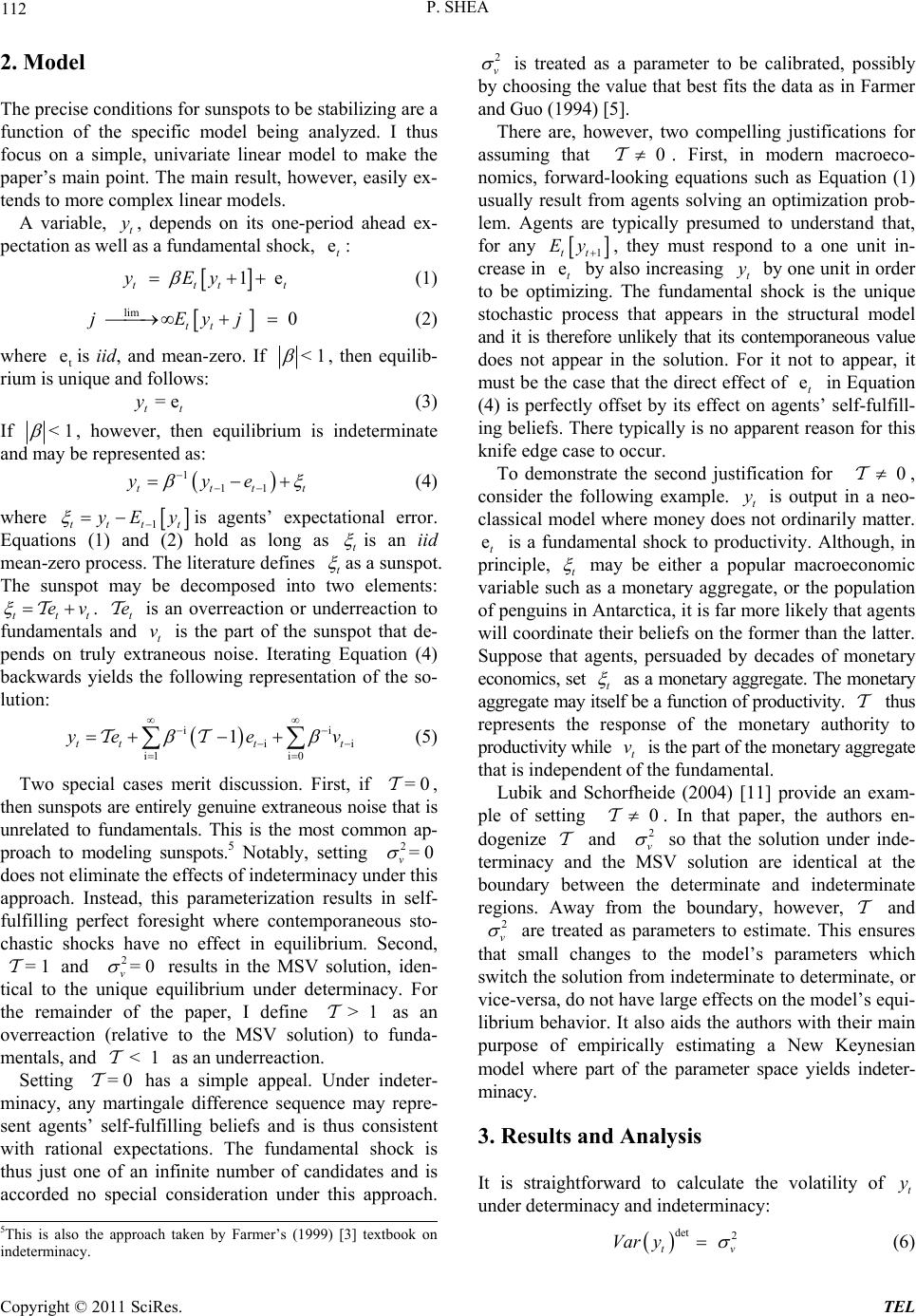 P. SHEA 112 2. Model The precise conditions for sunspo ts to be stabilizing are a function of the specific model being analyzed. I thus focus on a simple, univariate linear model to make the paper’s main point. The main result, however, easily ex- tends to more complex linear models. A variable, t, depends on its one-period ahead ex- pectation as well as a fundamental shock, : yet 1 e ttt yEy t (1) lim tt jEyj 0 (2) where tis iid, and mean-zero. If e< 1 , then equilib- rium is unique and follows: = e t yt (3) If < 1 , however, then equilibrium is indeterminate and may be represented as: 111ttt yye t (4) where 1tttt y Ey is agents’ expectational error. Equations (1) and (2) hold as long as t is an iid mean-zero process. The literature defines t as a sunspot. The sunspot may be decomposed into two elements: ttt ev e v . t is an overreaction or underreaction to fundamentals and t is the part of the sunspot that de- pends on truly extraneous noise. Iterating Equation (4) backwards yields the following representation of the so- lution: ii i i1 i0 1 ttt t yeev i (5) Two special cases merit discussion. First, if , then sunspots are entirely genuine extraneous noise that is unrelated to fundamentals. This is the most common ap- proach to modeling sunspots.5 Notably, setting does not eliminate the effects of indeterminacy under this approach. Instead, this parameterization results in self- fulfilling perfect foresight where contemporaneous sto- chastic shocks have no effect in equilibrium. Second, and results in the MSV solution, iden- tical to the unique equilibrium under determinacy. For the remainder of the paper, I define as an overreaction (relative to the MSV solution) to funda- mentals, and as an underreaction. = 0 2= 0 v 1 = 12 = 0 v < 1 > Setting has a simple appeal. Under indeter- minacy, any martingale difference sequence may repre- sent agents’ self-fulfilling beliefs and is thus consistent with rational expectations. The fundamental shock is thus just one of an infinite number of candidates and is accorded no special consideration under this approach. = 0 2 v is treated as a parameter to be calibrated, possibly by choosing the value that best fits the data as in Farmer and Guo (1994) [5]. There are, however, two compelling justifications for assuming that 0 . First, in modern macroeco- nomics, forward-looking equations such as Equation (1) usually result from agents solving an optimization prob- lem. Agents are typically presumed to understand that, for any 1tt Ey et , they must respond to a one unit in- crease in by also increasing t by one unit in order to be optimizing. The fundamental shock is the unique stochastic process that appears in the structural model and it is therefore unlikely that its contemporaneous value does not appear in the solution. For it not to appear, it must be the case that the direct effect of in Equation (4) is perfectly offset by its effect on agents’ self-fulfill- ing beliefs. There typically is no apparent reason for this knife edge case to occur. y et To demonstrate the second justification for 0 , consider the following example. t is output in a neo- classical model where money does not ordinarily matter. is a fundamental shock to productivity. Although, in principle, t y et may be either a popular macroeconomic variable such as a monetary aggregate, or the population of penguins in Antarctica, it is far more likely that agents will coordinate their beliefs on the former than the latter. Suppose that agents, persuaded by decades of monetary economics, set t as a monetary aggregate. The monetary aggregate may itself be a function o f productivity. thus represents the response of the monetary authority to productivity while t is the part of the monetar y aggregate that is independent of the fundamental. v Lubik and Schorfheide (2004) [11] provide an exam- ple of setting 0 2 v . In that paper, the authors en- dogenize and so that the solution under inde- terminacy and the MSV solution are identical at the boundary between the determinate and indeterminate regions. Away from the boundary, however, and 2 v are treated as parameters to estimate. This ensures that small changes to the model’s parameters which switch the solution from indeterminate to determinate, or vice-versa, do not have large effects on the model’s equi- librium behavior. It also aids the authors with their main purpose of empirically estimating a New Keynesian model where part of the parameter space yields indeter- minacy. 3. Results and Analysis It is straightforward to calculate the volatility of under determinacy and indeterminacy: t y 5This is also the approach taken by Farmer’s (1999) [3] textbook on indeterminacy. det 2 t Var yv (6) Copyright © 2011 SciRes. TEL 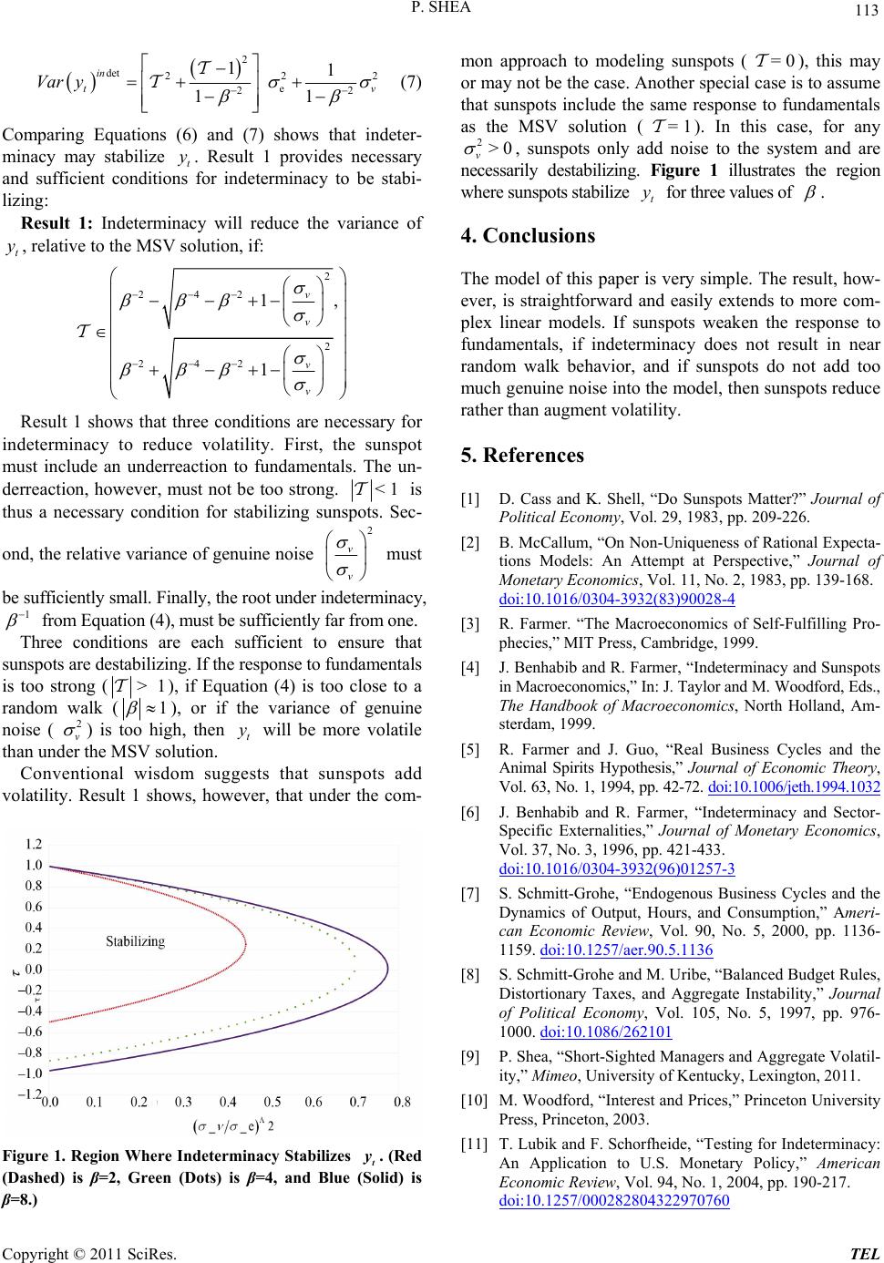 P. SHEA Copyright © 2011 SciRes. TEL 113 2 det 22 e 22 11 11 in t Var y2 v (7) mon approach to modeling sunspots (), this may or may not be the case. Another special case is to assume that sunspots include the same response to fundamentals as the MSV solution (). In this case, for any , sunspots only add noise to the system and are necessarily destabilizing. Figure 1 illustrates the region where sunspots stabilize for three values of = 0 = 1 t y 2>0 v . Comparing Equations (6) and (7) shows that indeter- minacy may stabilize t. Result 1 provides necessary and sufficient conditions for indeterminacy to be stabi- lizing: y Result 1: Indeterminacy will reduce the variance of , relative to the MSV solution, if: t y4. Conclusions 2 242 2 242 1, 1 v v v v The model of this paper is very simple. The result, how- ever, is straightforward and easily extends to more com- plex linear models. If sunspots weaken the response to fundamentals, if indeterminacy does not result in near random walk behavior, and if sunspots do not add too much genuine noise into the model, then sunspots reduce rather than augment v olatility. Result 1 shows that three conditions are necessary for indeterminacy to reduce volatility. First, the sunspot must include an underreaction to fundamentals. The un- derreaction, however, must not be too strong. < 1 is thus a necessary condition for stabilizing sunspots. Sec- 5. References [1] D. Cass and K. Shell, “Do Sunspots Matter?” Journal of Political Economy, Vol. 29, 1983, pp. 209-226. ond, the relative variance of genuine noise 2 v v must [2] B. McCallum, “On Non-Uniqueness of Rational Expecta- tions Models: An Attempt at Perspective,” Journal of Monetary Economics, Vol. 11, No. 2, 1983, pp. 139-168. doi:10.1016/0304-3932(83)90028-4 be sufficiently small. Fi nally, the root under indeterminacy, 1 from Equation (4), m ust be sufficiently far from one. [3] R. Farmer. “The Macroeconomics of Self-Fulfilling Pro- phecies,” MIT Press, Cambridge, 1999. Three conditions are each sufficient to ensure that sunspots are destabilizing. If the response to fundamentals is too strong (> 1), if Equation (4) is too close to a random walk (1 ), or if the variance of genuine noise (2 v ) is too high, then will be more volatile than under the MSV solution. t y [4] J. Benhabib and R. Farmer, “Indeterminacy and Sunspots in Macroeconomics,” In: J. Taylor and M. Wo odf ord, Eds., The Handbook of Macroeconomics, North Holland, Am- sterdam, 1999. [5] R. Farmer and J. Guo, “Real Business Cycles and the Animal Spirits Hypothesis,” Journal of Economic Theory, Vol. 63, No. 1, 1994, pp. 42-72. doi:10.1006/jeth.1994.1032 Conventional wisdom suggests that sunspots add volatility. Result 1 shows, however, that under the com- [6] J. Benhabib and R. Farmer, “Indeterminacy and Sector- Specific Externalities,” Journal of Monetary Economics, Vol. 37, No. 3, 1996, pp. 421-433. doi:10.1016/0304-3932(96)01257-3 [7] S. Schmitt-Grohe, “Endogenous Business Cycles and the Dynamics of Output, Hours, and Consumption,” Ameri- can Economic Review, Vol. 90, No. 5, 2000, pp. 1136- 1159. doi:10.1257/aer.90.5.1136 [8] S. Schmitt-Grohe and M. Uribe, “Balanced Budget Rules, Distortionary Taxes, and Aggregate Instability,” Journal of Political Economy, Vol. 105, No. 5, 1997, pp. 976- 1000. doi:10.1086/262101 [9] P. Shea, “Short-Sighted Managers and Aggregate Volatil- ity,” Mimeo, University of Kentucky, Lexington, 2011. [10] M. Woodford, “Interest and Prices,” Princeton University Press, Princeton, 2003. [11] T. Lubik and F. Schorfheide, “Testing for Indeterminacy: An Application to U.S. Monetary Policy,” American Economic Review, Vol. 94, No. 1, 2004, pp. 190-217. doi:10.1257/000282804322970760 Figure 1. Region Where Indeterminacy Stabilizes t y . (Red (Dashed) is β=2, Green (Dots) is β=4, and Blue (Solid) is β=8.) |