Solution for Rational Expectation Models Free of Complex Numbers

doi:10.4236/tel.2011.13011

Paper Menu >>

Journal Menu >>

Theoretical Economics Letters, 2011, 1, 47-52

doi:10.4236/tel.2011.13011 Published Online November 2011 (http://www.SciRP.org/journal/tel)

Solution for Rational Expectation Models

Free of Complex Numbers

Frank Hespeler

Institute for Forecasting and Macroeconomic Research, Tashkent, Uzbekistan

E-mail: [email protected]

Received July 2, 2011; revised August 25, 2011; accepted September 5, 2011

Abstract

This paper approaches the problem of the potential for complex-valued solutions within linear macroeco-

nomic models with rational expectations. It finds that these problems are associated with a specific solution

method for the underlying model. The paper establishes that the danger of complex-valued solutions always

can be eliminated by forcing those solutions to fulfill additional constraints. These constraints are essentially

restrictions on the degrees of freedoms in indeterminate solutions.

Keywords: Rational Expectation Models, Indeterminacy, Potentially Complex Coefficients

1. Introduction

Within the solution of dynamic economic models with

rational expectations regularly some kind of matrix de-

composition technique is employed in order to separate

the stable (generalized) eigenvalues from the unstable

(generalized) eigenvalues. Examples are the eigen de-

composition, the Schur decomposition or the generalized

Schur decomposition. All these decompositions share the

property that for real matrix polynomials it is sometimes

less costly to compute complex decompositions than real

decompositions. This raises the question whether we can

nevertheless assert real-valued solution paths. [1] shows

for the case of the eigen decomposition that this can be

achieved by choosing appropriate constants associated

with each eigenvalue. This paper discusses the same

question for the case of the generalized Schur decompo-

sition. It shows that while the structural properties of the

decomposition methods support real-valued solutions,

they do not always suffice to assert such solution paths.

In particular, the structural properes of the generalized

Schur decomposition can not assert real-valued solution

paths for the case that the model’s expectational error is

explained as a function of the exenous shocks to the

model as e.g. in [2]. Hence, in order to get a real-valued

solution of the model for this case, it is necessary to in-

troduce additional conditions to force the solution to the

real domain.

The paper develops such conditions. Of course this

requires some degrees of freedom within the solution of

the model, since a unique solution does not allow for the

development of additional conditions. Therefore the pa-

per applies to solutions of rational expectations models

which are characterized by indeterminacy. Within this

solution it attempts to use the available degrees of free-

dom to solve for a constellation, in which the coefficients

of endogenous and exogenous variables are forced into

the appropriately dimensioned real spaces . If

such a constellation exists, the entire solution of the

model is a real-valued one. To this purpose this paper

uses the fact that the product of two complex matrices

generates an imaginary part which consists in the sum of

the products of the real part of one matrix and the imagi-

nary one of the other matrix. Within this imaginary part

eventually complex-valued exogenous components can

be balanced by the imaginary part of the components

containing the degrees of freedom. Thus the product’s

imaginary part is set to zero. Applying this to the coeffi-

cient mentioned it can be guaranteed that the coefficient

is a real-valued matrix.

mn



The conditions obtained are sufficient conditions for

the existence of a real-valued solution. These conditions

built on the model’s transversality condition, which is

integrated into the model’s solution in a specific way that

does not allow any complex values for the model’s en-

dogenous variables. Thus, if necessary, the conditions

restrict the degrees of freedom available in the solution

further beyond the scope of restriction already obtained

by the mere integration of the transversality condition in

[3]. For the case that the transversality condition does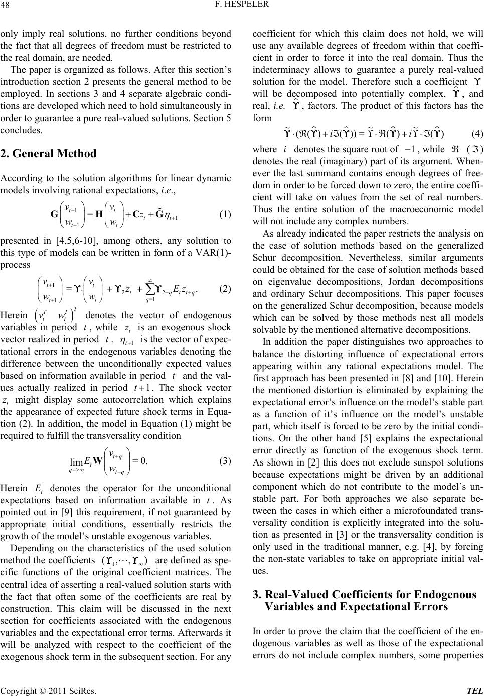

F. HESPELER

only imply real solutions, no further conditions beyond

the fact that all degrees of freedom must be restricted to

the real domain, are needed.

The paper is organized as follows. After this section’s

introduction section 2 presents the general method to be

employed. In sections 3 and 4 separate algebraic condi-

tions are developed which need to hold simultaneously in

order to guarantee a pure real-valued solutions. Section 5

concludes.

2. General Method

According to the solution algorithms for linear dynamic

models involving rational expectations, i.e.,





 



 

 

GHCG

 (1)

presented in [4,5,6-10], among others, any solution to

this type of models can be written in form of a VAR(1)-

process

122

= .

tqt









 



 

 





(2)

Herein denotes the vector of endogenous

variables in period , while is an exogenous shock

vector realized in period . 1t



vw tt





is the vector of expec-

tational errors in the endogenous variables denoting the

difference between the unconditionally expected values

based on information available in period and the val-

ues actually realized in period . The shock vector

t might display some autocorrelation which explains

the appearance of expected future shock terms in Equa-

tion (2). In addition, the model in Equation (1) might be

required to fulfill the transversality condition

1t

=0.

lim tq

qtq



 







W (3)

Herein t denotes the operator for the unconditional

expectations based on information available in t. As

pointed out in [9] this requirement, if not guaranteed by

appropriate initial conditions, essentially restricts the

growth of the model’s unstable exogenous variables.

Depending on the characteristics of the used solution

method the coefficients 1 are defined as spe-

cific functions of the original coefficient matrices. The

central idea of asserting a real-valued solution starts with

the fact that often some of the coefficients are real by

construction. This claim will be discussed in the next

section for coefficients associated with the endogenous

variables and the expectational error terms. Afterwards it

will be analyzed with respect to the coefficient of the

exogenous shock term in the subsequent section. For any

coefficient for which this claim does not hold, we will

use any available degrees of freedom within that coeffi-

cient in order to force it into the real domain. Thus the

indeterminacy allows to guarantee a purely real-valued

solution for the model. Therefore such a coefficient

(,, )







will be decomposed into potentially complex,





, and

real, i.e.





, factors. The product of this factors has the

form













(() ())=()()i i 



 

i1



(4)

where denotes the square root of , while



(



)

denotes the real (imaginary) part of its argument. When-

ever the last summand contains enough degrees of free-

dom in order to be forced down to zero, the entire coeffi-

cient will take on values from the set of real numbers.

Thus the entire solution of the macroeconomic model

will not include any complex numbers.

As already indicated the paper restricts the analysis on

the case of solution methods based on the generalized

Schur decomposition. Nevertheless, similar arguments

could be obtained for the case of solution methods based

on eigenvalue decompositions, Jordan decompositions

and ordinary Schur decompositions. This paper focuses

on the generalized Schur decomposition, because models

which can be solved by those methods nest all models

solvable by the mentioned alternative decompositions.

In addition the paper distinguishes two approaches to

balance the distorting influence of expectational errors

appearing within any rational expectations model. The

first approach has been presented in [8] and [10]. Herein

the mentioned distortion is eliminated by explaining the

expectational error’s influence on the model’s stable part

as a function of it’s influence on the model’s unstable

part, which itself is forced to be zero by the initial condi-

tions. On the other hand [5] explains the expectational

error directly as function of the exogenous shock term.

As shown in [2] this does not exclude sunspot solutions

because expectations might be driven by an additional

component which do not contribute to the model’s un-

stable part. For both approaches we also separate be-

tween the cases in which either a microfoundated trans-

versality condition is explicitly integrated into the solu-

tion as presented in [3] or the transversality condition is

only used in the traditional manner, e.g. [4], by forcing

the non-state variables to take on appropriate initial val-

ues.

3. Real-Valued Coefficients for Endogenous

Variables and Expectational Errors

In order to prove the claim that the coefficient of the en-

dogenous variables as well as those of the expectational

errors do not include complex numbers, some properties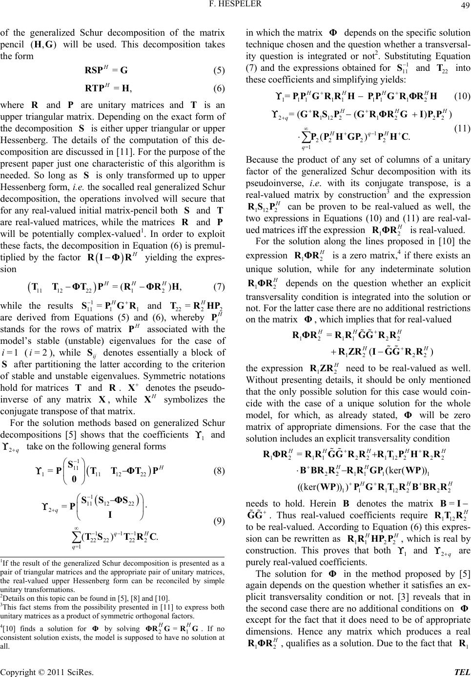

F. HESPELER 49

of the generalized Schur decomposition of the matrix

pencil will be used. This decomposition takes

the form

(,)HG

RSPG (5)

RTPH (6)

where and are unitary matrices and T is an

upper triangular matrix. Depending on the exact form of

the decomposition is either upper triangular or upper

Hessenberg. The details of the computation of this de-

composition are discussed in [11]. For the purpose of the

present paper just one characteristic of this algorithm is

needed. So long as is only transformed up to upper

Hessenberg form, i.e. the socalled real generalized Schur

decomposition, the operations involved will secure that

for any real-valued initial matrix-pencil both and T

are real-valued matrices, while the matrices and P

will be potentially complex-valued1. In order to exploit

these facts, the decomposition in Equation (6) is premul-

tiplied by the factor

R P



RI ΦR yielding the expres-

sion



11 122212

=() ,

HH H

TTΦTPR ΦRH (7)

while the results and 22 2

are derived from Equations (5) and (6), whereby

11 11

=H

SPGR



TRHP

stands for the rows of matrix

TR 

associated with the

model’s stable (unstable) eigenvalues for the case of

(), while ij denotes essentially a block of

after partitioning the latter according to the criterion

of stable and unstable eigenvalues. Symmetric notations

hold for matrices and . denotes the pseudo-

inverse of any matrix , while

=1i

=2i

X symbolizes the

conjugate transpose of that matrix.

For the solution methods based on generalized Schur

decompositions [5] shows that the coefficients 1



and

take on the following general forms

2q





111122





 





PTTΦTP

 (8)



11 1222

111

22 22222

().

















SSΦS

TS TRC



(9)

in which the matrix depends on the specific solution

technique chosen ande question whether a transversal-

ity question is integrated or not2. Subs

(7) and the expressiobtained for and into

these coefficients anplifying yields:

ons

d sim

tituting Equation



S22

11111 1112

HH HH

PPGRHPPGR ΦRH (10)

211221222

2222

= ( ( ))

().

HqH











GRS PGRΦRG IPP

PPHGPP HC



(11)



Because the product of any set of columns of a

factor of the generalized Schur decomposition with its

pseudoinverse, i.e. with its conjugate transpose, is a

real-valued matrix by construction3 and the expre

unitary

ssion

112 2

RS P can be proven to be real-valued as well, the

two expressions in Equations (10) and (11) are real-val-

ued matrices iff the expression 12

RΦR is real-valued.

For the solution along the lines proposed in [10] the

expression 12

RΦR is a zero matrix,4 if there exists an

olution, while for any indeterminate solution

unique s

RΦR depends on the question whether an explicit

transversality condition is intego the solution or rated int

not. For the latter case there are no additional restrictions

on the matriich implies that for real-valued

12 1122

12 22

()

HH H





RΦRRRGGRR

RZRIGG RR



the expression 12

x Φ, wh

RZR need to be real-valued as well.

Without presenting details, it should be only mentioned

that the only psible solution for this case would coios

case of a

ich, as

cide with the unique solution for the whole

model, for wh already stated, will be zero

riate dim

matrix of appropensions. For the case that the

solution includes an explicit transversality condition

12 1122112222

22 11 11

11 112222

(ker())

((ker()))

HHHH H





 





RΦRRRGGRRRTPHRR

BBRRRR GPWP

WPPGR TRBBRR



needs to hold. Herein B denotes the matrix =





 . Thus real-valoefficients require ued c112 2

RT R

pres-to be real

sion can

-valued. Accog to Equation (6

be rewritten as

rdin) this ex

11 22

RR HPP

that both 

, which is

truction. This pro and

real by

consves 1





are

purely real-valued coefficients.

e solution for Φ in the method proposed]

again depends on the question whether it satisfies an ex-

plicit transversality condition or not. [3] reveals that in

the second case there are no additiona conditions on Φ

except for the fact that it does need toe of apriate

dimensions. Hence any matrix

1If the result of the generalized Schur decomposition is presented as a

air of triangular matrices and the appropriate pair of unitary matrices,

the real-valued upper Hessenberg form can be reconciled by simple

unitary transformations.

2Details on this topic can be found in [5], [8] and [10].

3This fact stems from the possibility presented in [11] to express both

unitary matrices as a product of symmetric orthogonal factors.

4[10] finds a solution for Φ by solving 21

. If no

consistent solution exists, the model is supposed to have no solution at

all.

ΦRG RG

Th by [5

bprop

which produces a real

RΦR, qualifies as a solution. Due to the fact that 1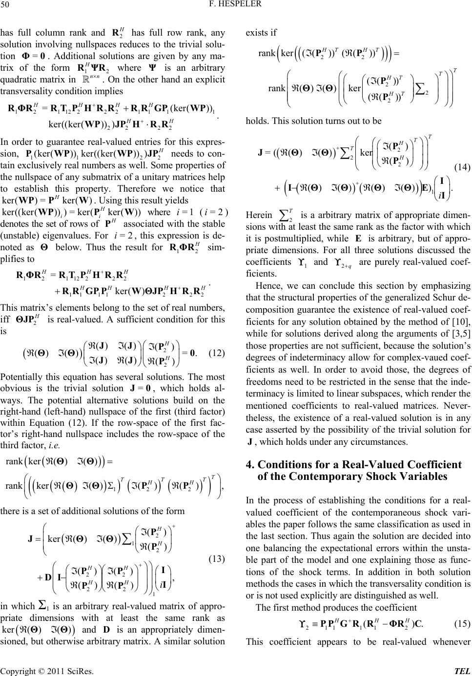

F. HESPELER

has full column rank and 2

R has full row rank, any

solution involving nullspaces reduces to the trivial solu-

tion =Φ0. Additional solutions are given by any m

trix of the form 12

RΨR where Ψ is an arbitrary

quadratic matrix in nn

. On the other hand an explicit

trans

vers

ality condition implies

12112222 1111

22 22

=(ker())

ker((ker()))

HHHH





RΦRRTPHRRRRGP WP

WPJPHR R

In order to guarantee-valued entries for this expres-

sion, 11

(ker( ))ker((ker( )))

real

PWP WPJP needs to con-

tain exclusively real numbers as welm

ker

Presult yields

t of row

l. So

of a unitary m

ore we

e properties of

atrices help

notice that

the nullspace

to establish t

) =WP

s the se

of any subm

is property

( )W. Usi

s of

atrix

. There

ng this

ker(

ker((ker())) = ker(ker())

WPPW where =1i (=2i)

denote

P associated with the stable

(unstable) eigenvalues. For =2i, this expression is de-

noted as Θ below. Thus the result for 12

RΦR sim-

plifies to

11 122 2

er()

12 11222

RR .



RR GPPWΘJPHR R

This matrix’s elements belonhe set of real numbers,

iff 2

RΦTPH

g to t

ΘJP s real-valued. A sufficient con

()

s. The

t-hand (le

within Equation

ght-ha

dition for this

ybuild on the

righft-hace of tst (third factor)

w-spof the fi

tor’s rind cludes the row-space of the



()

)()

potential alterna

nd) nu

(12). If the

nullspace i

() ()

( =.

() ()





 





ΘΘ 0









utions

he fir

ace





tive sol

llspa

Potentially this equation has several solutions. The most

obvious is the trivial solution =J0, which holds al-

rst fac-

third factor, i.e.



rankker( )()ΘΘ







122

rankker()()()

TTT





 









ΘΘ PP,

there is a set of additional solutions of the form











y m













d m

trix. A si

()

ker ()

()





 







() ()

HHi











 



DI I

( )(

()



ΘΘ

rbitrary

with at

and D

rwise arbitrar

)







in which Σ1

dime

( )

d, but ot

(13

is an aeal-valueatrix of appro-

priate nsions least the same rank as

is an apropriately dimen-

amilar solution

exists if



ker( )ΘΘ

sione he













rank ker(())(())

(( ))

rank()()ker

(( ))

HT HT

 







 











ΘΘ



holds. This solution turns out to be



()

= (()()ker









()

()()()()).



 







 



IΘΘ ΘΘEI



(14)

Herein





 

P

JΘΘ



is a arbitrary matrix of appropriate dimen-

sions with at least the same rank as the factor with which

it is postmplied, while is arbitrary, but of appro-

lutions discussed the

coefficients

ulti E

priate dimensions. For all three so



and 2q





are purely real-valued coef-

ficients.

Hence, we can conclude this section by emphasizing

that the structural properties of the generalized Schu

composition guarantee the existence of real-valued coef-

ficients for any solution obtained by the method of [10],

r solut

lim line

tio both solution

r de-

while foions derived along the arguments of [3,5]

those properties are not sufficient, because the solution’s

degrees of indeterminacy allow for complex-vaued coef-

ficients as well. In order to avoid those, the degrees of

freedoms need to be restricted in the sense that the inde-

terminacy is ited to ar subspaces, which render the

mentioned coefficients to real-valued matrices. Never-

theless, the existence of a real-valued solution is in any

case asserted by the possibility of the trivial solution for

J, which holds under any circumstances.

4. Conditions for a Real-Valued Coefficient

of the Contemporary Shock Variables

In the process of establishing the conditions for a real-

valued coefficient of the contemporaneous shock vari-

ables the paper follows the same classification as used in

the last section. Thus again the solution are decided into

one balancing the expectational errors within the unsta-

ble part of the model and one explaining those as func-

ns of the shock terms. In addition in

methods the cases in which the transversality condition i

or is not used explicitly are distinguished as well.

The first method produces the coefficient

211 112

().

HHH

PPG RRΦRC (15)

This coefficient appears to be real-valued whenever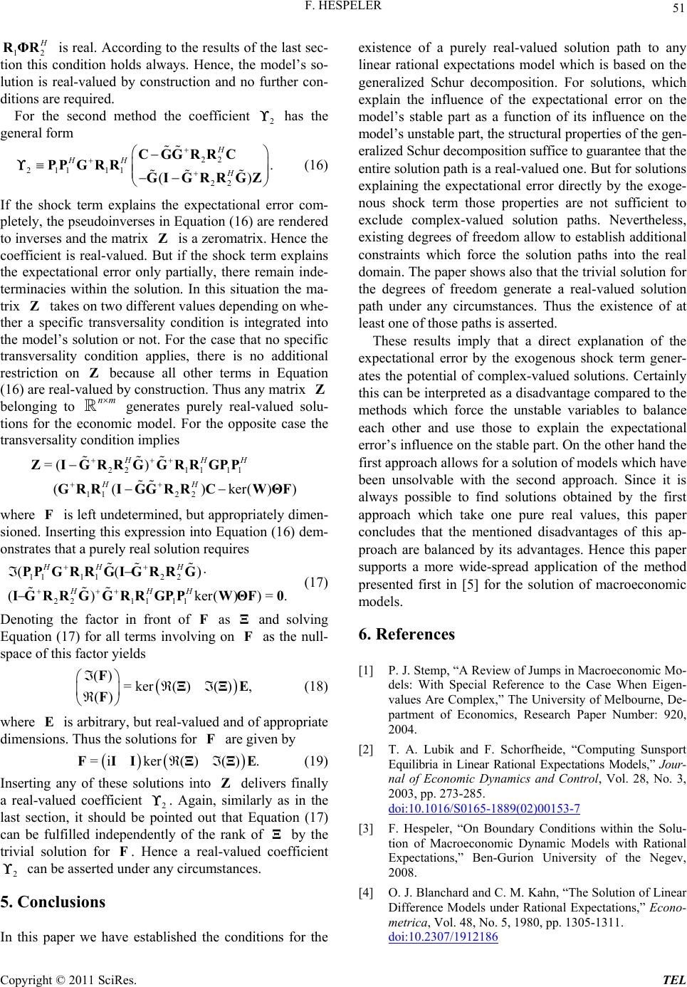

F. HESPELER 51

RΦR is real. According to the results of the last sec-

tion this condition holds always. Hence, the model’s so-

lution is real-valued by construction and no further con-

ditions are required.

For the second method the coefficient 2

 has the

general form

H





CGGRRC



211 11()











PP GR R

GIGRRGZ

 





(16)

If the shock term explains the expectational error com

to invers

e soltion. In this situation the ma-

tri ing

tran integrated into

the model’s solution or For the case that no specific

condition applies, there is no

onbecauseother terms in Equation

l onas the null-

space of this factor yields

(18)

ven by

Inserting any of these solutions into delivers

in il

a real-valued coefficient

can be asserted y circumce

the

existence of a purely real-valued solution

ntire solution path is a real-valued one. But for solutions

ctational error directly by the exoge-

properties are not sufficient to

l values, this paper

, pp. 273-285.

doi:10.1016/S0165-1889(02)00153-7



pletely, the pseudoinverses in Equation (16) are rendered

es and the matrix Z is a zeromatrix. Hence the

coefficient is real-valued. But if the shock term explains

the expectational error only partially, there remain inde-

terminacies within thu

sversality condition is

not.

all

x Z takes on two different values depend on whe-

ther a specific

transversality

restriction

additional

(16) are real-valued by construction. Thus any matrix Z

belonging to mn

 generates purely real-valued solu-

tions for the economic model. For the opposite case the

transversality condition implies

2211 11

1122

=( )

(()ker())

HHH









ZIGRRGGRR GPP

GRRI GGRRCWΘF





where F is left undetermined, but appropriately dimen-

sioned. Inserting this expression into Equation (16) dem-

onstrates that a purely real solution requires

111 122

2211 11

(()

() ker())=.

HH H

HHH







PPG RRGIGRRG

IGRR GRR GPPWΘF0



 (1

Denoting the factor in front of F as Ξ and solving

Equation (17) for all terms invo





ving F



() =ker()( ),



 



FΞΞE

()



where E is arbitrary, but real-valued and of appropriate

dimensions. Thus the solutions for F are gi

 

=iker()() .FIIΞΞE (19)

finally

stan

a real-valued coefficient 2

. Aga, simarly as in the

last section, it should be pointed out that Equation (17)

can be fulfilled independently of the rankf Ξ by the

trivial solution for F. Hence

r an



undes.

5. Conclusions

In this paper we have established the conditions for

path to any

linear rational expectations model whh is based on the

generalized Schur decomsition. For solutions, which

explain the influence of the expectational error on the

model’s stable part as a function of its influence on the

model’s unstable part, the structural properties of the gen-

elized Schur decomposition suffice to guarantee that the

explaining the expe

ous shock term those n

exclude complex-valued solution paths. Nevertheless,

existing degrees of freedom allow to establish additional

constraints which force the solution paths into the real

domain. The paper shows also that the trivial solution for

the degrees of freedom generate a real-valued solution

path under any circumstances. Thus the existence of at

least one of those paths is asserted.

These results imply that a direct explanation of the

expectational error by the exogenous shock term gener-

ates the potential of complex-valued solutions. Certainly

this can be interpreted as a disadvantage compared to the

methods which force the unstable variables to balance

each other and use those to explain the expectational

error’s influence on the stable part. On the other hand the

first approach allows for a solution of models which have

been unsolvable with the second approach. Since it is

always possible to find solutions obtained by the first

approach which take one pure rea

ncludes that the mentioned disadvantages of this ap-

proach are balanced by its advantages. Hence this paper

supports a more wide-spread application of the method

presented first in [5] for the solution of macroeconomic

models.

6. References

[1] P. J. Stemp, “A Review of Jumps in Macroeconomic Mo-

dels: With Special Reference to the Case When Eigen-

values Are Complex,” The University of Melbourne, De-

partment of Economics, Research Paper Number: 920,

2004.

[2] T. A. Lubik and F. Schorfheide, “Computing Sunsport

Equilibria in Linear Rational Expectations Models,” Jour-

nal of Economic Dynamics and Control, Vol. 28, No. 3,

2003

On Boundary Conditions within the Solu-

tion of Macroeconomic Dynamic Models with Rational

, Vol. 48, No. 5, 1980, pp. 1305-1311.

doi:10.2307/1912186

[3] F. Hespeler, “

Expectations,” Ben-Gurion University of the Negev,

2008.

[4] O. J. Blanchard and C. M. Kahn, “The Solution of Linear

Difference Models under Rational Expectations,” Econo-

metrica

F. HESPELER

/s10614-007-9114-2

[5] F. Hespeler, “Solution Algprithm to a Class of Monetary

Rational Equilibrium Macromodels with Optimal Mone-

tary Policy,” Computational Economics, Vol. 31, No. 3,

2008, pp. 207-223. doi:10.1007

olution of Singular[6] R. G. King and M. W. Watson, “The S

Linear Difference Systems under Rational Expectations,”

International Economic Review, Vol. 39, No. 4, 1998, pp.

1015-1028. doi:10.2307/2527350

[7] R. G. King and M. W. Watson, “System Reduction and

6911923

Solution Algorithms for Singular Linear Difference Sys-

tems under Rational Expectations,” Computational Eco-

nomics, Vol. 20, No. 1-2, 2002, pp. 57-68.

doi:10.1023/A:102057

ctations Model,” Jour-

[8] P. Klein, “Using the Generalized Schur form to Solve a

Multivariate Linear Rational Expe

nal of Economic Dynamics and Control, Vol. 24, No. 10,

2000, pp. 1405-1423.

doi:10.1016/S0165-1889(99)00045-7

[9] P. Kowal, “An Algorithm for Solving Srb

Rational Expectations Model,” Eitrary Linear

conWPA, 2005.

[10] C. A. Sims, “Solving Linear Rational Expectations Mod-

els,” Computational Economics, Vol. 20, No. 1-2, 2002,

pp. 1-20. doi:10.1023/A:1020517101123

[11] C. Moler and G. Stewart, “An Algorith

Matrix Eigenvalue Problems,” SIAM m for Generalized

Journal on Nume-

rical Analysis, Vol. 10, No. 2, 1973, pp. 241-256.

doi:10.1137/0710024