

Paper Menu >>
Journal Menu >>
 Journal of Signal and Information Processing, 2011, 2, 287-291 doi:10.4236/jsip.2011.24041 Published Online November 2011 (http://www.SciRP.org/journal/jsip) Copyright © 2011 SciRes. JSIP 1 Least Squares Matrix Algorithm for State-Space Modelling of Dynamic Systems Juuso T. Olkkonen1, Hannu Olkkonen2 1VTT Technical Research Centre of Finland, Espoo, Finland; 2Department of Applied Physics, University of Eastern Finland, Kuopio, Finland. Email: Juuso.[email protected] Received October 4th, 2011; revised November 1st, 2011; accepted November 10th, 2011. ABSTRACT This work presents a novel least squares matrix algorithm (LSM) for the analysis of rapidly changing systems using state-space modelling. The LSM algorithm is based on the Hankel structured data matrix representation. The state transition matrix is updated without the use of any forgetting function. This yields a robust estimation of model pa- rameters in the presence of noise. The computational complexity of the LSM algorithm is comparab le to the speed of the conventional recursive least squares (RLS) algorithm. The knowledge of the state transition matrix enables feasible numerical operators such as interpolation, fractional differentiation and integration. The usefulness of the LSM algo- rithm was proved in the analysis of the neuroelectric signal waveforms. Keywords: State-Space Modell i ng, Dynamic System Anal ysis, EEG 1. Introduction Estimation of the state of the dynamic systems has been a research object for many years since the innovation of the Kalman filter (KF) [1-4]. The time-varying autoregressive models are useful in analysis of relatively slowly chang- ing dynamic systems. The adaptive least mean squares (LMS) algorithm has been extensively applied in the analysis of various biomedical and industrial systems [5,6]. A disadvantage of the LMS algorithm is the poor adaptation in systems with abrupt changes. The more fastly adapting recursive least squares (RLS) algorithm [7], Kohonen neural network [8], extended Kalman filter (EKF) [9] and many other approaches have recently intr- oduced for robust and accurate space-state modelling of the highly varying dynamic systems. The computational power of the most of the algorithms is based on the recur- sive updating of the model parameters and matrices. Usu- ally this is solved by using a forgetting function, which gives the higher weight to the most recent data values. In this work we describe the least squares matrix (LSM) algorithm, where the state-space model is based on the Hankel structured data matrix formulation. In the updating algorithm, no forgetting function is used. 2. Theoretical Considerations 2.1. Dynamic State-Space Model We consider the dynamic state-space model 1,, nnnn nn X FXy CX w (1) where the state vector 1 N n X , the state transition matrix N N n F and the vector 1 100 0 N C . The scalar 11 n w n y y n is a random zero mean observa- tion noise. The signal consists of measurem- ents at time increments , where is the sampling period. Let us define the data vector 1nn and the Hankel structured data matrix 11 n y tnTn 1 0,1,2,T T nN Yy H as 11 12 2 12 11 . nn nM nn nN n nN nNnNM nn nM yy y yy y H yy y YY Y 2 (2) The subscript in n and n nY H refers to the most recent data point n. The least squares estimate of the state transition matrix comes from y n G 1 1 1 #1 1 () , nnn TT nnnnn nn nn HFH FHHHH HH RC (3) where the pseudoinverse matrix 1 #TT nnnn HHHH N N nn CH , nand The rank of the state transition 1 TN nn RHH . TNN n H N  Least Squares Matrix Algorithm for State-Space Modelling of Dynamic Systems 288 matrix n F defines the system order. In many appli- cations the state transition matrix should be evaluated at T intervals. In complex dynamic systems the dimension of the state transition matrix is high and the computation of the pseudoinverse matrix # n H is time consuming. Instead, by partitioning the state transition matrix n F into n and matrices we introduce a novel algorithm for updating the R1 n C 1 n C and n matrices and for the computation of the state transition matrix R n F . 2.2. Computation of the 1 n C Matrix Using the data vector representation (2) the matrix can be written as n C 11 T n Y 1 T nM Y nM Y 2 1 TT nn nn nM YY Y 1 . T nM 1 n U n H n CC 1 TT nM Y 2 n Y n Y 1 CH Y n U Y 1 nM Y T n T Y Y (4) The uptake of the n matrix is obtained by adding a new term and subtracting the oldest term as C 11 . T n n Y (5) A key idea in this work is that we write the last two terms as 1 1 1 1 nnM n nM YY Y 11 n, n V (6) where and N N n V nn 11 n V U . Now we obtain the updated matrix as 1n C nn CC 1 1 1. n CC n V 1 () n CU U n n I 22 . 1 (7) The matrix inversion lemma yields the inverse matrix 1 11 1 () nn n n U CC VV 1 nn C , (8) where the identity matrix By denoting I 2 N nn n U 1 n VCV CC n C 11 U n ZI 1 n C we have . (9) nn nn Z For fast computation of the n Z matrix the product 12 N nn is first computed and then the inverse matrix . In Equation (9) the product is first computed. n C 1N RH RV nn n IR CU 1 nn U 2 nn n RH n R n nn H RY 22 2.3. Computation of the Matrix n 11 n 2 1 TT n T n T nM Y Y Y R TT n Y n Y The matrix can be written as n R 1 T n T n nM H YY YY 1 n . 1 21 , T n V nM Y nM Y R (10) The matrix can be updated as 1211 1 n nnM nM n R Y Y U (11) where the same notations as in Equation (6) have been used. 2.4. Computation of the n F Matrix The uptake of the state transition matrix 1 nnn F RC co- mes from 1 111 11 1 1 11 . nnn nnnn nnn nnnn nnn FRC RUVC CUZ FFUZUVC (12) For fast computation the products 2N nn FU and 12 1 N nn VC are first computed. The uptake of the state transition matrix needs five matrix multiplications dimen- sioned as 2NN N and four matrix multiplicati- ons dimensioned as 22NN or 2.2NN Thus the computational complexity of the algorithm is 2 52ON 44ON. 3. Applications of the LSM Algorithm 3.1. State-Space Filtering The knowledge of the state transition matrix n F enables the filtering of the measurement signal based on the prediction n y 1 ˆnnn H FH (13) The state-space filtered signal can be obtained as a mean of the antidiagonal elements. We may define the filtered data matrix as ˆn y 11 12 2 12 ˆˆ ˆ ˆˆ ˆ ˆ. ˆˆ ˆ nn nM nn nM n nN nNnNM yy y yy y H yy y 2 (14) In the following we describe several matrix operators based on the state transition matrix. In all computations the filtered data matrix (14) is applied. 3.2. Numerical Signal Processing The knowledge of the state transition matrix n F enables the numerical signal processing of the state-space filtered signal. In the following we develop matrix operators based on the state transition matrix for numerical inter- polation, differentiation and integration of the measure- ment signal. The eigenvalue decomposition of the state transition matrix is 1 nnnn F UDU , where D12 diag NN nN and N N n U . Based on (14) we have a result 1 1 1 ˆˆ ˆ ˆˆ , nnnnnnn nnnnnn HFHUDUH ˆ n H UDU HFH (15) Copyright © 2011 SciRes. JSIP 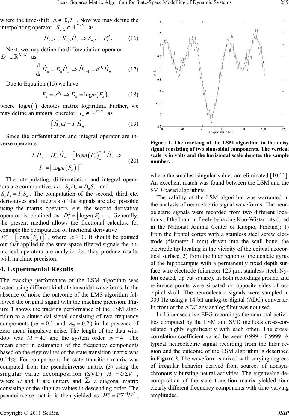 Least Squares Matrix Algorithm for State-Space Modelling of Dynamic Systems289 where the time-shift 0,T , . Now we may define the interpolating operator N N n S ˆˆ as ,, . nnnnn H SH SF (16) Next, we may define the differentiation operator N N n D as 1 dˆˆˆ. d n D nnn nˆ n H DHHe H t (17) Due to Equation (15) we have log , n D nnn F eD mF (18) where denotes matrix logarithm. Further, we may define an integral operator logm N N n I as ˆ d nn ˆ n . H tIH (19) Since the differentiation and integral operator are in- verse operators 1 1 1 ˆˆ ˆ log log nnn nnn nn IHD HmFH ImF (20) The interpolating, differentiation and integral opera- tors are commutative, i.e. nn nn and nnn n . The computation of the second, third etc. derivatives and integrals of the signals are also possible using the matrix operators, e.g. the second derivative operator is obtained as n . Generally, the present method allows the fractional calculus, for example the computation of fractional derivative n SD DS 2log n D SI IS log n D 2 mF mF , where 0 . It should be pointed out that applied to the state-space filtered signals the nu- merical operators are analytic, i.e. they produce results with machine precision. 4. Experimental Results The tracking performance of the LSM algorithm was tested using different kind of sinusoidal waveforms. In the absence of noise the outcome of the LMS algorithm fol- lowed the original signal with the machine precision. Fig- ure 1 shows the tracking performance of the LSM algo- rithm to a sinusoidal signal consisting of two frequency components (10.1 and 20.2 ) in the presence of zero mean impulsive noise. The length of the data win- dow was and the system order 40M4.N The mean error in estimation of the frequency components based on the eigenvalues of the state transition matrix was 0.14%. For comparison, the state transition matrix was computed from the pseudoinverse matrix (3) using the singular value decomposition (SVD) T n H UV # n , where U and V are unitary and a diagonal matrix consisting of the singular values in descending order. The pseudoinverse matrix is then yielded as 1T H V U , sample number volts Figure 1. The tracking of the LSM algorithm to the noisy signal consisting of two sinusoidal components. The vertical scale is in volts and the horizontal scale denotes the sample number. where the smallest singular values are eliminated [10,11]. An excellent match was found between the LSM and the SVD-based algorithms. The validity of the LSM algorithm was warranted in the analysis of neuroelectric signal waveforms. The neur- oelectric signals were recorded from two different loca- tions of the brain in freely behaving Kuo-Wistar rats (bred in the National Animal Center of Kuopio, Finland): 1) from the frontal cortex with a stainless steel screw elec- trode (diameter 1 mm) driven into the scull bone, the electrode tip locating in the vicinity of the epipial neocor- tical surface, 2) from the hilar region of the dentate gyrus of the hippocampus with a permanently fixed depth sur- face wire electrode (diameter 125 μm, stainless steel, Ny- lon coated, tip cut square). In both recordings ground and reference points were situated on opposite sides of oc- cipital skull. The neuroelectric signals were sampled at 300 Hz using a 14 bit analog-to-digital (ADC) converter. In front of the ADC any analog filter was not used. In 16 consecutive EEG recordings the neuronal activi- ties computed by the LSM and SVD methods cross-cor- related highly significantly with each other. The cross- correlation coefficient varied between 0.999 - 0.9999. A typical neuroelectric signal recording from the hilar re- gion and the outcome of the LSM algorithm is described in Figure 2. The waveform is mixed with varying degrees of irregular behavior derived from sources of nonsyn- chronously bursting neural activities. The eigenvalue de- composition of the state transition matrix yielded four clearly different frequency components with time-varying amplitudes. Copyright © 2011 SciRes. JSIP 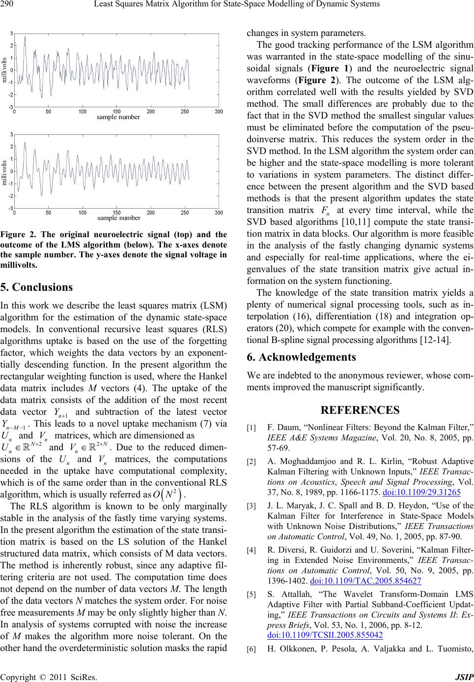 Least Squares Matrix Algorithm for State-Space Modelling of Dynamic Systems 290 sample number sample number millivolt smillivolt s Figure 2. The original neuroelectric signal (top) and the outcome of the LMS algorithm (below). The x-axes denote the sample number. The y-axes denote the signal voltage in millivolts. 5. Conclusions In this work we describe the least squares matrix (LSM) algorithm for the estimation of the dynamic state-space models. In conventional recursive least squares (RLS) algorithms uptake is based on the use of the forgetting factor, which weights the data vectors by an exponent- tially descending function. In the present algorithm the rectangular weighting function is used, where the Hankel data matrix includes M vectors (4). The uptake of the data matrix consists of the addition of the most recent data vector 1n and subtraction of the latest vector 1. This leads to a novel uptake mechanism (7) via and n matrices, which are dimensioned as and Y nM Y n U n U V 2N2 N n V V. Due to the reduced dimen- sions of the n U and n matrices, the computations needed in the uptake have computational complexity, which is of the same order than in the conventional RLS algorithm, which is usually referred as. 2 ON The RLS algorithm is known to be only marginally stable in the analysis of the fastly time varying systems. In the present algorithm the estimation of the state transi- tion matrix is based on the LS solution of the Hankel structured data matrix, which consists of M data vectors. The method is inherently robust, since any adaptive fil- tering criteria are not used. The computation time does not depend on the number of data vectors M. The length of the data vectors N matches the system order. For noise free measurements M may be only slightly higher than N. In analysis of systems corrupted with noise the increase of M makes the algorithm more noise tolerant. On the other hand the overdeterministic solution masks the rapid changes in system parameters. The good tracking performance of the LSM algorithm was warranted in the state-space modelling of the sinu- soidal signals (Figure 1) and the neuroelectric signal waveforms (Figure 2). The outcome of the LSM alg- orithm correlated well with the results yielded by SVD method. The small differences are probably due to the fact that in the SVD method the smallest singular values must be eliminated before the computation of the pseu- doinverse matrix. This reduces the system order in the SVD method. In the LSM algorithm the system order can be higher and the state-space modelling is more tolerant to variations in system parameters. The distinct differ- ence between the present algorithm and the SVD based methods is that the present algorithm updates the state transition matrix n F at every time interval, while the SVD based algorithms [10,11] compute the state transi- tion matrix in data blocks. Our algorithm is more feasible in the analysis of the fastly changing dynamic systems and especially for real-time applications, where the ei- genvalues of the state transition matrix give actual in- formation on the system functioning. The knowledge of the state transition matrix yields a plenty of numerical signal processing tools, such as in- terpolation (16), differentiation (18) and integration op- erators (20), which compete for example with the conven- tional B-spline signal processing algorithms [12-14]. 6. Acknowledgements We are indebted to the anonymous reviewer, whose com- ments improved the manuscript significantly. REFERENCES [1] F. Daum, “Nonlinear Filters: Beyond the Kalman Filter,” IEEE A&E Systems Magazine, Vol. 20, No. 8, 2005, pp. 57-69. [2] A. Moghaddamjoo and R. L. Kirlin, “Robust Adaptive Kalman Filtering with Unknown Inputs,” IEEE Transac- tions on Acoustics, Speech and Signal Processing, Vol. 37, No. 8, 1989, pp. 1166-1175. doi:10.1109/29.31265 [3] J. L. Maryak, J. C. Spall and B. D. Heydon, “Use of the Kalman Filter for Interference in State-Space Models with Unknown Noise Distributions,” IEEE Transactions on Automatic Control, Vol. 49, No. 1, 2005, pp. 87-90. [4] R. Diversi, R. Guidorzi and U. Soverini, “Kalman Filter- ing in Extended Noise Environments,” IEEE Transac- tions on Automatic Control, Vol. 50, No. 9, 2005, pp. 1396-1402. doi:10.1109/TAC.2005.854627 [5] S. Attallah, “The Wavelet Transform-Domain LMS Adaptive Filter with Partial Subband-Coefficient Updat- ing,” IEEE Transactions on Circuits and Systems II: Ex- press Briefs, Vol. 53, No. 1, 2006, pp. 8-12. doi:10.1109/TCSII.2005.855042 [6] H. Olkkonen, P. Pesola, A. Valjakka and L. Tuomisto, Copyright © 2011 SciRes. JSIP  Least Squares Matrix Algorithm for State-Space Modelling of Dynamic Systems Copyright © 2011 SciRes. JSIP 291 “Gain Optimized Cosine Transform Domain LMS Algo- rithm for Adaptive Filtering of EEG,” Computers in Bi- ology and Medicine, Vol. 29, 1999, pp. 129-136. doi:10.1016/S0010-4825(98)00046-8 [7] E. Eweda, “Comparison of RLS, LMS, and Sign Algo- rithms for Tracking Randomly Time-Varying Channels,” IEEE Transactions on Signal Processing, Vol. 43, No. 11, 1994, pp. 2937-2944. doi:10.1109/78.330354 [8] D. Niebur and A. J. Germond, “Power System Static Se- curity Assessment Using the Kohonen Neural Network Classifier,” IEEE Transactions on Power Systems, Vol. 7, No. 2, 1992, pp. 865-872. doi:10.1109/59.141797 [9] D.-J. Jwo and S.-H. Wang, “Adaptive Fuzzy Strong Tracking Extended Kalman Filtering for GPS Naviga- tion,” IEEE Sensors Journal, Vol. 7, No. 5, 2007, pp. 778-789. doi:10.1109/JSEN.2007.894148 [10] S. Park, T. K. Sarkar and Y. Hua, “A Singular Value Decomposition-Based Method for Solving a Determinis- tic Adaptive Problem,” Digital Signal Processing, Vol. 9, No. 1, 1999, pp. 57-63. doi:10.1006/dspr.1998.0331 [11] T. J. Willink, “Efficient Adaptive SVD Algorithm for MIMO Applications,” IEEE Transactions on Signal Pro- cessing, Vol. 56, No. 2, 2008, pp. 615-622. doi:10.1109/TSP.2007.907806 [12] M. Unser, A. Aldroubi and M. Eden, “B-Spline Signal Processing. I. Theory,” IEEE Transactions on Signal Pro- cessing, Vol. 41, No. 2, 1993, pp. 821-833. doi:10.1109/78.193220 [13] M. Unser, A. Aldroubi and M. Eden, “B-Spline Signal Processing. II. Efficiency Design and Applications,” IEEE Transactions on Signal Processing, Vol. 41, No. 2, 1993, pp. 834-848. doi:10.1109/78.193221 [14] J. T. Olkkonen and H. Olkkonen, “Fractional Time-Shift B-Spline Filter,” IEEE Signal Processing Letters, Vol. 14, No. 10, 2007, pp. 688-691. doi:10.1109/LSP.2007.896402 |