Inhomogeneous material property assignment and ori-entation definition of transverse isotropy of femur

doi:10.4236/jbise.2009.26060

Paper Menu >>

Journal Menu >>

Vol.2, No.6, 419-424 (2009)

doi:10.4236/jbise.2009.26060

JBiSE

Inhomogeneous material property assignment and

orientation definition of transv erse isotropy of femur

Hai-Sheng Yang1,2, Tong-Tong Guo1, Jian-Huang Wu2, Xin Ma2,3

1Biomechanics Laboratory, Department of Mathematics and Natural Science, Harbin Institute of Technology Shenzhen Graduate

School, Shenzhen, China; 2Shenzhen Institute of Advanced Integration Technology, Chinese Academy of Sciences/The Chinese Uni-

versity of Hong Kong, Shenzhen, China; 3Harbin Institute of Technology, Harbin, China.

Email: [email protected]

Received 28 April 2009; revised 10 June 2009; accepted 12 June 2009.

ABSTRACT

The finite element method has been increas-

ingly adopted to study the biomechanical be-

havior of biologic structures. Once the finite

element mesh has been generated from CT data

set, the assignment of bone tissue’s material

properties to each element is a fundamental

step in the generation of individualized or sub-

ject-specific finite element models. The aim of

this work is to simulate the inhomogeneous and

anisotropic material properties of femur using

the finite element method. A program is devel-

oped to read a CT data set as well as the finite

element mesh generated from it, and to assign

to each element of the mesh the material prop-

erties derived from the bone tissue density at

the element location. Moreover, for cancellous

bone in femoral neck and cortical bone in fe-

moral stem, the principal orientations of trans-

verse isotropy were defined based on the tra-

becular structures and the haversian system

respectively.

Keywords: Finite Element; Material Property; In-

homogeneous; Transve rse Isotropy; Femur

1. INTRODUCTION

The determination of the mechanical stresses in human

bones is of great importance in both research and clinical

practice. Since the stresses in bones cannot be measured

non-invasively in vivo, an effective way to estimate

them is through the finite element (FE) an alysis which is

widely used in academic research and clinical applica-

tions, such as the theory of bone remodeling [1], the

design of pro sthesis [2 ] and th e ev aluation of factur e risk

[3]. In early period the methods used to get bone geome-

try and mechanical properties were inaccurate and some-

times highly invasive and destructive. It is well known

that CT images can provide fairly accurate quantitative

information on bone geometry based on high contrast

between the bone tissue and the soft tissue around [4,5].

Moreover, it has been demonstrated that CT numbers are

almost linearly correlated with apparent density of bio-

logic tissues [6]. Good empirical relationships have been

established experimentally between density and me-

chanical properties of bone tissues [7,8].

In early studies, if a generic bone model was con-

structed, then the mechanical properties of the different

bone tissues were usually derived from average values

reported in published experimental studies [9]. For an

individualized or subject-specific model, however, me-

chanical properties should be derived from CT data. It

has been shown that the stress distribution of a bone is

strongly related to the mechanical p roperties distribution

in the bone tissue [10], and the mechanical properties of

bone have been showed to depend on the subject, anat-

omic location, orientation, biological processes and time.

Hence, it is important to find an effective method to

properly map the material properties derived from CT

data into finite element models.

The CT data can be regarded as a three-dimensional

scalar field (related to the tissue density) sampled over a

regular grid. If the finite element mesh is generated

starting from the same data, the mesh and the density

distribution are perfectly registered in space. The only

problem is how to account for this inhomogeneous dis-

tribution of material properties in to the FE model. Many

approaches were proposed in literature to perform this

task [11,12,13,14,15,16,17,18,19]. However, these algo-

rithms only simulated the inhomogeneity of bone, and

the isotropic material property assignment was adopted

without considering the orien tation of material. Since the

bone material is widely recognized as being anisotropic

rather than isotropic [8,20], the FE simulation of inho-

mogeneity and isotropy cannot reflect the actual charac-

teristics of bone structure. The aim of this study is to

simulate the inhomogeneous and anisotropic material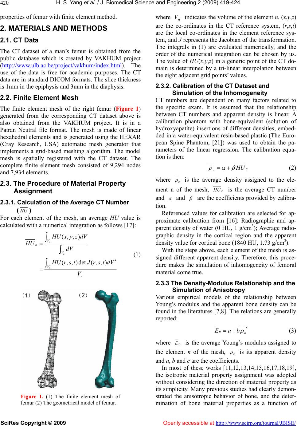

H. S. Yang et al. / J. Biomedical Science and Engineering 2 (2009) 419-424

420

properties of femur with finite element method.

2. MATERIALS AND METHODS

2.1. CT Data

The CT dataset of a man’s femur is obtained from the

public database which is created by VAKHUM project

(http://www.ulb.ac.b e/proj ect/vakhu m/index.h tml). The

use of the data is free for academic purposes. The CT

data are in standard DICOM formats. The slice thickness

is 1mm in the epiphysis and 3mm in the diaphysis.

2.2. Finite Element Mesh

The finite element mesh of the right femur (Figure 1)

generated from the corresponding CT dataset above is

also obtained from the VAKHUM project. It is in a

Patran Neutral file format. The mesh is made of linear

hexahedral elements and is generated using the HEXAR

(Cray Research, USA) automatic mesh generator that

implements a grid-based meshing algorithm. The model

mesh is spatially registered with the CT dataset. The

complete finite element mesh consisted of 9,294 nodes

and 7,934 elements.

2.3. The Procedure of Material Property

Assignment

2.3.1. Calculation of the Average CT Number

(HU )

For each element of the mesh, an average HU value is

calculated with a numerical integration as follows [17]:

(,,)

(,,)det (,,)

HUxyzdV

HU dV

Urst JrstdV











 (1)

Figure 1. (1) The finite element mesh of

femur (2) The geometrical model of femur.

where indicates the volume of the element n, (x,y,z)

are the co-ordinates in the CT reference system, (r,s,t)

are the local co-ordinates in the element reference sys-

tem, and J represents the Jacob ian of the transformation.

The integrals in (1) are evaluated numerically, and the

order of the numerical integration can be chosen by us.

The value of HU(x,y,z) in a generic point of the CT do-

main is determined by a tri-linear interpolation between

the eight adjacent grid points’ values.

2.3.2. Calibration of the CT Dataset and

Simulation of the Inhomogeneity

CT numbers are dependent on many factors related to

the specific exam. It is assumed that the relationship

between CT numbers and apparent density is linear. A

calibration phantom with bone-equivalent (solution of

hydroxyapatite) insertions of different densities, embed-

ded in a water-equivalent resin-based plastic (The Euro-

pean Spine Phantom, [21]) was used to obtain the pa-

rameters of the linear regression. The calibration equa-

tion is then:



 (2)

where n



is the average density assigned to the ele-

ment n of the mesh, n

HU is the average CT number

and



and



are the coefficients provided by calibra-

tion.

Referenced values for calibration are selected for ap-

proximate calibration from [16]: Radiographic and ap-

parent density of water (0 HU, 1 g/cm3); Average radio-

graphic density in the cortical region and the apparent

density value for cortical bone (1840 HU, 1.73 g/cm3).

With the steps above, each element of the mesh is as-

signed different apparent density. Therefore, this proce-

dure makes the simulation of inhomogeneity of femoral

material come true.

2.3.3 The Density-Modulus Relationship and the

Simulation of Anisotropy

Various empirical models of the relationship between

Young’s modulus and the apparent bone density can be

found in the literatures [7,8]. The relations are generally

reported:

Eab



 (3)

where n

E is the average Young’s modulus assigned to

the element n of the mesh, n



is its apparent density

and a, b and c are the coefficients.

In most of these works [11,12,13,14,15,16,17,18,19],

the isotropic material property assignment was adopted

without considering th e direction of material property as

its simplicity. Many prev ious studies had clearly demon-

strated the anisotropic behavior of bone, and the deter-

mination of bone material properties as a function of

H. S. Yang et al. / J. Biomedical Science and Engineering 2 (2009) 419-424

421

direction is the essential requirement [22]. The axial

direction is defined according to the Haversian osteons

of the cortical bone and according to the spatial main

direction of the trabecular structures of cancellous bone.

The relationship between bone material properties and

apparent density is given by [8]:

coincide with the structure of bone.

As we know, bone structure is customarily recognized

as confirming to ‘wolff’s law’ which is essentially the

observation that bone changes its external shape and

internal architecture in response to stresses acting on it.

Thus, the structure of bone (or material orientation)

strongly coincides with the principal stress track. The

directions of the femoral neck and stem can be approxi-

mately regarded as stress track in femur.

 Cortical bone:

1.57 3.09

12 3

1213 23

12 1121323

2314 ,2065 ,

0.58, 0.32,

/ 2(1),3300;

EE E

GE GG







 



 

(4) Femoral bone can be recognized as transversely iso-

tropic material. According to the cortical bone structure

in femoral stem and cancellous bone structure in femoral

neck, the principal material orientation of cancellous

bone is defined by the direction of the trabecular struc-

tures and the principal material orientation of cortical

bone by the direction of the haversian system.

 Cancellous bone:

1.78 1.64

12 3

1213 23

12 1121323

1157 ,1094 ,

0.58, 0.32,

/ 2(1),110;

EE E

GE GG







 



 

(5)

3. RESULTS

where E is the Young’s modulus (MPa), G the shear

modulus (MPa),



is the apparent density (g/cm3),



the Poisson’s ratio. All parameters are set in elemental

Cartesian coordinate system of Patran (MSC, USA).

3.1. Material Properties Distribution

This material assignment procedure produces 165 dif-

ferent material cards. The distribution of the material

properties in femur are shown in Figure 2. The maxi-

mum and minimum values for apparent density and elas-

tic modulus are listed in Ta b l e 1. The maximum values

are corresponding to the Mat-1 and the minimum to

Mat-165 as a result of the definitio n in the program. The

numbers of elements for each material property card are

showed in Figure 3.

This procedure may, theoretically, lead to a different

material card (Mat) for each element of the mesh, which

may result in computational problems with those codes

that can handle a limited number of materials. We can

reduce the number of materials by choosing a



threshold. Then the maximum computed value of the

elastic modulus, is assigned to the material Mat-1.

All the elements with are assigned the

material Mat-1. Mat-2 is characterized by the maximum

E of the remaining elements and so on until the whole

set of the model material is defined. In this paper, the

threshold

max

)( max EEE 

 is taken as 50 MPa.

3.2. The FE Simulation of Transversely

Isotropic Material Property

Figure 2 only showed the inhomogeneous distribution

of material properties. After separating the femoral stem

and neck, th e prin cipa l material orientations for elements

in neck and stem are defined respectively. Figure 4 il-

lustrates the vector form of the principal orientations in

femoral neck. Figure 5 presents the vector form of the

principal orientations in femoral stem.

A program was developed to read the original data in-

cluding CT data, finite element mesh data and some pa-

rameters and then to implement the procedure described

above. In this way, each element is assigned different

density, elastic modulus and Poisson’s ratio. At last, a

finite element mesh provided with the assigned material

properties is written out in a Patran Neutral file format. 4. DISCUSSION

Every element of the finite element model has its own

element coordinate system used to determine the mate-

rial’s principal axe of this element. As the element coor-

dinate systems vary from element to element, the prin-

cipal material orientations need to be defined so as to

As is well-known, it is of significance to explore the

biomechanical behavior of bone. FE analysis has been

adopted by many researchers based on CT data that can

provide useful information on the geometrical topology

Table 1. Material properties of femur (the unit for density is g/cm3, and for elastic modulus is MPa).

Material properties Maximum Minimum



1.787 0.686

E1 (E2) 5755.799 591.512

E3 12410.846 1026.157

Openly accessible at

H. S. Yang et al. / J. Biomedical Science and Engineering 2 (2009) 419-424

422

Figure 2. Right femur with different material properties

mapped on it, observed from different angles of view.

Figure 3. The number of elements for each material property card.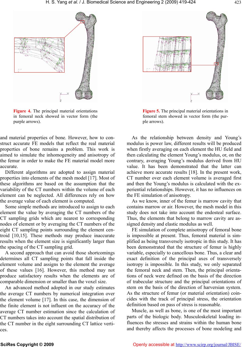

H. S. Yang et al. / J. Biomedical Science and Engineering 2 (2009) 419-424

423

Figure 4. The principal material orientations

in femoral neck showed in vector form (the

purple arrows).

Figure 5. The principal material orientations in

femoral stem showed in vector form (the pur-

ple arrows).

and material properties of bone. However, how to con-

struct accurate FE models that reflect the real material

properties of bone remains a problem. This work is

aimed to simulate the inhomogeneity and anisotropy of

the femur in order to make the FE material model more

accurate.

As the relationship between density and Young’s

modulus is power law, different results will be produced

when firstly averaging on each element the HU field and

then calculating th e element Young’s modulus, or, on the

contrary, averaging Young’s modulus derived from HU

value. It has been demonstrated that the latter can

achieve more accurate results [18]. In the present work,

CT number over each element volume is averaged first

and then the Young’s modulus is calculated with the ex-

periential relationships. However, it has no influences on

the FE simulation of anisotropy.

Different algorithms are adopted to assign material

properties into elements of the mesh model [17]. Most of

these algorithms are based on the assumption that the

variability of the CT numbers within the volume of each

element can be neglected. All differences rely on how

the average value of each element is computed. As we know, inner of the femur is marrow cavity that

contains marrow or air. Howev er, the mesh model in this

study does not take into account the endosteal surface.

Thus, the elements that belong to marrow cavity are as-

signed density and elastic modulus as well.

Some simple methods are introduced to assign to each

element the value by averaging the CT numbers of the

CT sampling grids which are nearest to corresponding

nodes of element or by averaging the CT numbers of the

eight CT sampling points surrounding the element cen-

troid [10,15]. These methods may produce inaccurate

results when the element size is significantly larger than

the spacing of the CT sampling grid.

FE simulation of complete anisotropy of femoral bone

is impossible at present. Thus, femoral material is sim-

plified as being transv ersely isotrop ic in this study. It has

been demonstrated that the structure of femur is highly

variable, especially to cancellous bone. Thus, a clear and

exact definition of the principal axes of transversely

isotropy is impossible. In this study, we only separated

the femoral neck and stem. Then, the principal orienta-

tions of neck were defined on the basis of the direction

of trabecular structure and the principal orientations of

stem on the basis of the direction of harversian system.

As the structure of femur (or material orientation) coin-

cides with the track of principal stress, the orientation

definition based on pass of stress is reasonable.

A second approach that can avoid those shortcomings

determines all CT sampling points that fall inside the

element volume and assigns to the element the average

of these values [16]. However, this method may not

produce satisfactory results when the elements are of

comparable dimension or smaller than the voxel size.

An advanced method adopted in our study estimates

the average CT numbers by numerical integration over

the element volume [17]. In this case, the dimension of

the finite element is not influent on the accuracy of the

average CT number estimation since the calculation of

CT numbers takes into account the spatial distribution of

the CT number in the eight surrounding CT lattice verti-

ces.

Muscle, as well as bone, is one of the most important

parts of the biologic body. Musculoskeletal loading in-

fluences the stresses and strains within the human bone

and thereby affects the processes of bone modeling and

Openly accessible at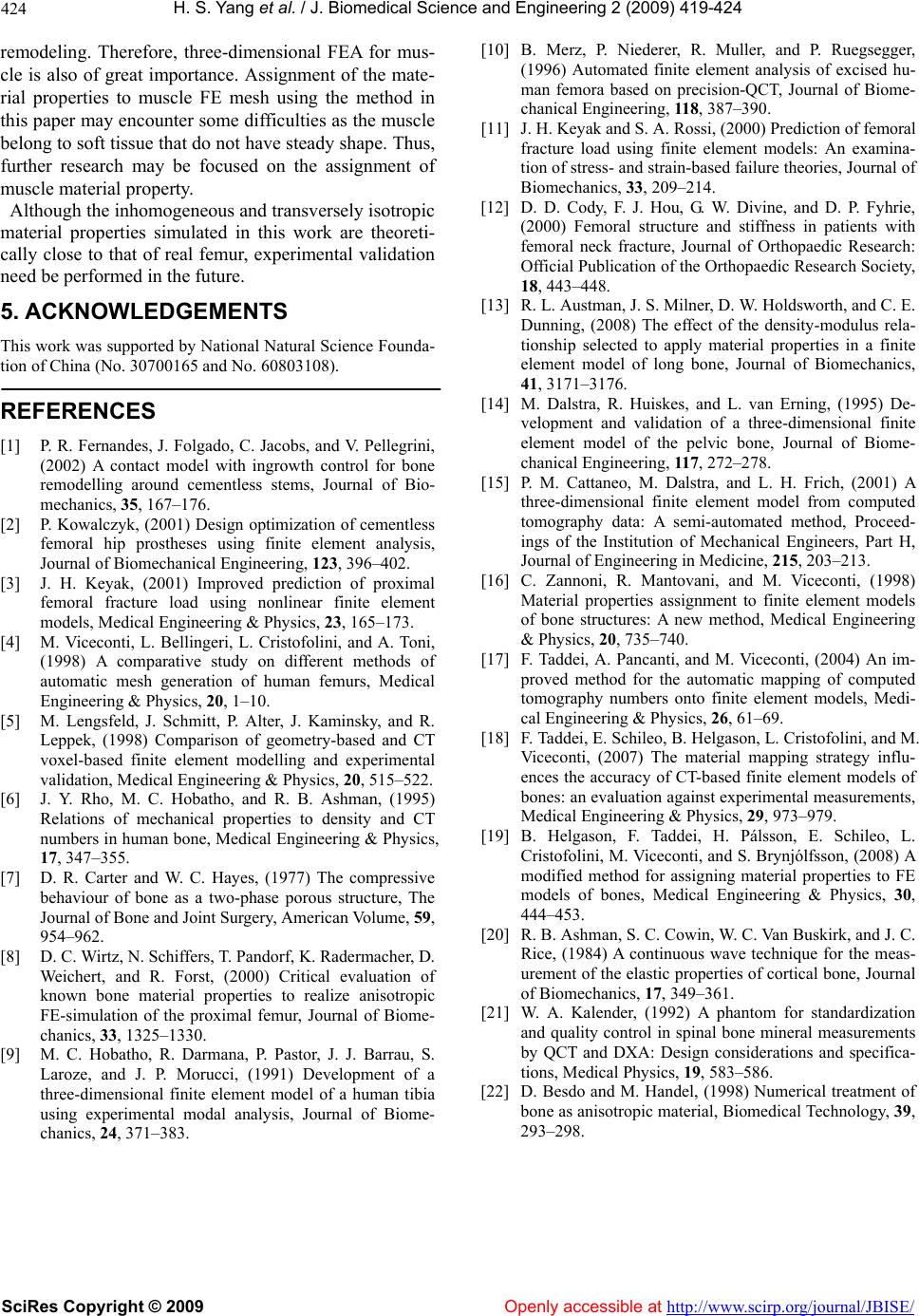

H. S. Yang et al. / J. Biomedical Science and Engineering 2 (2009) 419-424

424

remodeling. Therefore, three-dimensional FEA for mus-

cle is also of great importance. Assignment of the mate-

rial properties to muscle FE mesh using the method in

this paper may encounter some difficulties as the muscle

belong to soft tissue that do not have steady shape. Thus,

further research may be focused on the assignment of

muscle material property.

Although the inhomogen eous and transv ersely iso tropic

material properties simulated in this work are theoreti-

cally close to that of real femur, experimental validation

need be performed in the future.

5. ACKNOWLEDGEMENTS

This work was supported by National Natural Science Founda-

tion of China (No. 30700165 and No. 60803108).

REFERENCES

[1] P. R. Fernandes, J. Folgado, C. Jacobs, and V. Pellegrini,

(2002) A contact model with ingrowth control for bone

remodelling around cementless stems, Journal of Bio-

mechanics, 35, 167–176.

[2] P. Kowalczy k, (2001) Design optimization of cementless

femoral hip prostheses using finite element analysis,

Journal of Biomechanical Engineering, 123, 396–402.

[3] J. H. Keyak, (2001) Improved prediction of proximal

femoral fracture load using nonlinear finite element

models, Medical Engineering & Physics, 23, 165–173.

[4] M. Viceconti, L. Bellingeri, L. Cristofolini, and A. Toni,

(1998) A comparative study on different methods of

automatic mesh generation of human femurs, Medical

Engineering & Ph ysics, 20, 1–10.

[5] M. Lengsfeld, J. Schmitt, P. Alter, J. Kaminsky, and R.

Leppek, (1998) Comparison of geometry-based and CT

voxel-based finite element modelling and experimental

validation, Medical Engineering & Physics, 20, 515–522.

[6] J. Y. Rho, M. C. Hobatho, and R. B. Ashman, (1995)

Relations of mechanical properties to density and CT

numbers in human bone, Medical Engineering & Physics,

17, 347–355.

[7] D. R. Carter and W. C. Hayes, (1977) The compressive

behaviour of bone as a two-phase porous structure, The

Journal of Bone and Joint Surgery, American Volume, 59,

954–962.

[8] D. C. Wirtz, N. Schiffers, T. Pandorf, K. Radermacher, D.

Weichert, and R. Forst, (2000) Critical evaluation of

known bone material properties to realize anisotropic

FE-simulation of the proximal femur, Journal of Biome-

chanics, 33, 1325–1330.

[9] M. C. Hobatho, R. Darmana, P. Pastor, J. J. Barrau, S.

Laroze, and J. P. Morucci, (1991) Development of a

three-dimensional finite element model of a human tibia

using experimental modal analysis, Journal of Biome-

chanics, 24, 371–383.

[10] B. Merz, P. Niederer, R. Muller, and P. Ruegsegger,

(1996) Automated finite element analysis of excised hu-

man femora based on precision-QCT, Journal of Biome-

chanical Engineering, 118, 387–390.

[11] J. H. Keyak and S. A. Rossi, (2000) Prediction of femoral

fracture load using finite element models: An examina-

tion of stress- and strain-based failure theories, Journal of

Biomechanics, 33, 209–214.

[12] D. D. Cody, F. J. Hou, G. W. Divine, and D. P. Fyhrie,

(2000) Femoral structure and stiffness in patients with

femoral neck fracture, Journal of Orthopaedic Research:

Official Publication of the Orthopaedic Research Society,

18, 443–448.

[13] R. L. Austman, J. S. Milner, D. W. Holdsworth, and C. E.

Dunning, (2008) The effect of the density-modulus rela-

tionship selected to apply material properties in a finite

element model of long bone, Journal of Biomechanics,

41, 3171–3176.

[14] M. Dalstra, R. Huiskes, and L. van Erning, (1995) De-

velopment and validation of a three-dimensional finite

element model of the pelvic bone, Journal of Biome-

chanical Engineering, 117, 272–278.

[15] P. M. Cattaneo, M. Dalstra, and L. H. Frich, (2001) A

three-dimensional finite element model from computed

tomography data: A semi-automated method, Proceed-

ings of the Institution of Mechanical Engineers, Part H,

Journal of Engineering in Medicine, 215, 203–213.

[16] C. Zannoni, R. Mantovani, and M. Viceconti, (1998)

Material properties assignment to finite element models

of bone structures: A new method, Medical Engineering

& Physics, 20, 735–740.

[17] F. Taddei, A. Pancanti, and M. Viceconti, (2004) An im-

proved method for the automatic mapping of computed

tomography numbers onto finite element models, Medi-

cal Engineering & Physics, 26, 61–69.

[18] F. Taddei, E. Schileo, B. Helgason, L. Cristofolini, and M.

Viceconti, (2007) The material mapping strategy influ-

ences the accuracy of CT-based finite element models of

bones: an evaluation against experimental measurements,

Medical Engineering & Physics, 29, 973–979.

[19] B. Helgason, F. Taddei, H. Pálsson, E. Schileo, L.

Cristofolini, M. Viceconti, and S. Brynjólfsson, (2008) A

modified method for assigning material properties to FE

models of bones, Medical Engineering & Physics, 30,

444–453.

[20] R. B. Ashman, S. C. Cowin, W. C. Van Buskirk, and J. C.

Rice, (1984) A continuous wave technique for the meas-

urement of the elastic properties of cortical bone, Journal

of Biomechanics, 17, 349–361.

[21] W. A. Kalender, (1992) A phantom for standardization

and quality control in spinal bone mineral measurements

by QCT and DXA: Design considerations and specifica-

tions, Medical Physics, 19, 583–586.

[22] D. Besdo and M. Handel, (1998) Numerical treatment of

bone as anisotropic material, Biomedical Technology, 39,

293–298.