Fault Detection and Isolation Based on Neural Networks Case Study: Steam Turbine

doi:10.4236/epe.2011.34062

Paper Menu >>

Journal Menu >>

Energy and Power En gi neering, 2011, 3, 513-516

doi:10.4236/epe.2011.34062 Published Online September 2011 (http://www.SciRP.org/journal/epe)

Fault Detection and Isolation Based on Neural Networks

Case Study: Steam Turbine

Djamel Benazzouz, Samir Benammar, Smail Adjerid

Solid Mechanic and Systems Laboratory (LMSS), M’Hamed Bougara University, Boumerdès, Algeria

E-mail: [email protected]

Received February 9, 2011; revised March 20, 2011; accepted April 8, 2011

Abstract

The real-time fault diagnosis system is very important for steam turbine generator set due serious fault re-

sults in a reduced amount of electricity supply in power plant. A novel real-time fault diagnosis system is

proposed by using Levenberg-Marquardt algorithm related to tuning parameters of Artificial Neural Network

(ANN). The model of novel fault diagnosis system by using ANN are built and analyzed. Cases of the diag-

nosis are simulated. The results show that the real-time fault diagnosis system is of high accuracy and quick

convergence. It is also found that this model is feasible in real-time fault diagnosis. The steam turbine is used

as a power generator by SONELGAZ, an Algerian company located at Cap Djinet town in Boumerdes dis-

trict. We used this turbine as our main target for the purpose of this analysis. After deep investigation, while

keeping our focus on the most sensitive parts within the turbine, the weakest and the strongest points of the

system were identified. Those are the points mostly adequate for failure simulations and at which the de-

signed system will be better positioned for irregularities detection during the production process.

Keywords: Failure, Diagnosis, Artificial Neural Networks, Isolation, Steam Turbine

1. Introduction

The first role of the industrial diagnosis is to increase the

availability of the industrial installations to reduce the

direct and indirect maintenance costs of the production

equipments. The direct costs of this maintenance are

mainly those related to the various spare parts. On the

other hand, the indirect costs are essentially due to the

off line production [1,2]. The increase repair time influ-

ences negatively on the indirect maintenance costs.

The objective of this paper is to minimize this waiting

time for detecting the failure in the industrial installa-

tions. The proposed model will supervise the system,

detect and localize any faulty in real time. An important

characteristic of the proposed model is that it has the

possibility of detecting and locating several failing points

at the same time. For example: an increase in the vibra-

tion level in the four landings of the turbine. The data

vectors for the training in the Artificial Neural Network

(ANN) model are intervals limited by two values, mini-

mum and maximum. The used symbol “1” represents a

normal functioning and the symbol “–1” represents a

failure situation. The training algorithm used for the

network is the Levenberg-Marquardt algorithm, the choice

of this algorithm is that it gives a fast training of the

ANN compared to the other algorithms of decent of gra-

dient [3,4]. The programming was completely developed

under MATLAB 7.5.

2. Steam Turbine Presentation

The study case concerns a steam turbine of an Algerian

electrical production thermal plant SONELGAZ located

at Cap-Djinet, Boumerdes. The turbine transforms the

thermal energy contained in the vapor coming from the

boiler into a rotation movement of the tree. Mechanical

work obtained is used to actuate the alternator. It is

composed of three bodies, HP body (High Pressure), MP

body (Average Pressure) and BP body (Low Pressure). It

has a power and a nominal number of revolutions of 176

MW and 3000 rpm respectively. The line of tree rests on

four landings, each one of these landings thus carries two

relative vibration sensors, it is the total of eight sensors

on all the line of tree, but for model simplification we

consider only four sensors. The maximum value of rela-

tive vibrations that can be supported by the system is 120

μm. Figure 1 represents the supervision and placement

sensors site in the landings turbine.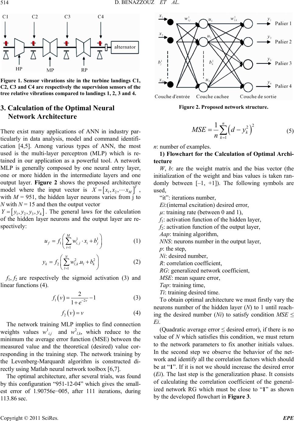

D. BENAZZOUZ ET AL.

514

Figure 1. Sensor vibrations site in the turbine landings C1,

C2, C3 and C4 are respectively the supervision sensors of the

tree relative vibrations compared to landings 1, 2, 3 and 4.

3. Calculation of the Optimal Neural

Network Architecture

There exist many applications of ANN in industry par-

ticularly in data analysis, model and command identifi-

cation [4,5]. Among various types of ANN, the most

used is the multi-layer perceptron (MLP) which is re-

tained in our application as a powerful tool. A network

MLP is generally composed by one neural entry layer,

one or more hidden in the intermediate layers and one

output layer. Figure 2 shows the proposed architecture

model where the input vector is ,

with M = 951, the hidden layer neurons varies from j to

N with N = 15 and then the output vector



,, T

Xxx x







1234

,,,Yyyyy. The general laws for the calculation

of the hidden layer neurons and the output layer are re-

spectively:

ij ij

uf wxb





















(1)

klkl

yf wub











 (2)

f1, f2 are respectively the sigmoid activation (3) and

linear functions (4).



fv e



 (3)





(4)

The network training MLP implies to find connection

weights values w1i,j and w

2l,k, which reduce to the

minimum the average error function (MSE) between the

measured value and the theoretical (desired) value cor-

responding in the training step. The network training by

the Levenberg-Marquardt algorithm is constructed di-

rectly using Matlab neural network toolbox [6,7].

The optimal architecture, after several trials, was found

by this configuration “951-12-04” which gives the small-

est error of 1.90756e−005, after 111 iterations, during

113.86 sec.

Figure 2. Proposed network structure.





SEd y

n



 (5)

n: number of examples.

1) Flowchart for the Calculation of Optimal Archi-

tecture

W, b: are the weight matrix and the bias vector (the

initialization of the weight and bias values is taken ran-

domly between [–1, +1]). The following symbols are

used,

“it”: iterations number,

Ei:(internal excitation) desired error,

µ: training rate (between 0 and 1),

f1: activation function of the hidden layer,

f2: activation function of the output layer,

Aap: training algorithm,

NNS: neurons number in the output layer,

p: the step,

Ni: desired number,

R: correlation coefficient,

RG: generalized network coefficient,

MSE: mean square error,

Tap: training time,

Ti: training desired time.

To obtain optimal architecture we must firstly vary the

neurons number of the hidden layer (N) to 1 until reach-

ing the desired number (Ni) to satisfy condition MSE ≤

Ei.

(Quadratic average error ≤ desired error), if there is no

value of N which satisfies this condition, we must return

to the network parameters to fix another initials values.

In the second step we observe the behavior of the net-

work and identify all the correlation factors which should

be at “1”. If it is not we should increase the desired error

(Ei). The last step is the generalization phase. It consists

of calculating the correlation coefficient of the general-

ized network RG which must be close to “1” as shown

by the developed flowchart in Figure 3.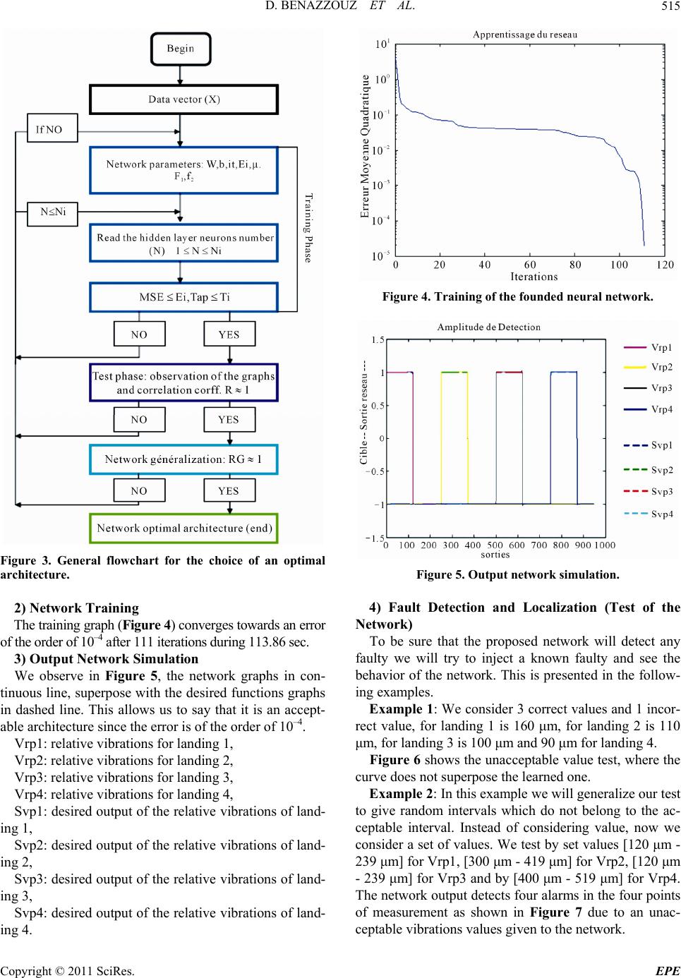

D. BENAZZOUZ ET AL.515

Figure 3. General flowchart for the choice of an optimal

architecture.

2) Network Training

The training graph (Figure 4) converges towards an error

of the order of 10–4 after 111 iterations during 113.86 sec.

3) Output Network Simulation

We observe in Figure 5, the network graphs in con-

tinuous line, superpose with the desired functions graphs

in dashed line. This allows us to say that it is an accept-

able architecture since the error is of the order of 10–4.

Vrp1: relative vibrations for landing 1,

Vrp2: relative vibrations for landing 2,

Vrp3: relative vibrations for landing 3,

Vrp4: relative vibrations for landing 4,

Svp1: desired output of the relative vibrations of land-

ing 1,

Svp2: desired output of the relative vibrations of land-

ing 2,

Svp3: desired output of the relative vibrations of land-

ing 3,

Svp4: desired output of the relative vibrations of land-

ing 4.

Figure 4. Training of the founded neur al ne twork.

Figure 5. Output network simulation.

4) Fault Detection and Localization (Test of the

Network)

To be sure that the proposed network will detect any

faulty we will try to inject a known faulty and see the

behavior of the network. This is presented in the follow-

ing examples.

Example 1: We consider 3 correct values and 1 incor-

rect value, for landing 1 is 160 μm, for landing 2 is 110

μm, for landing 3 is 100 μm and 90 μm for landing 4.

Figure 6 shows the unacceptable value test, where the

curve does not superpose the learned one.

Example 2: In this example we will generalize our test

to give random intervals which do not belong to the ac-

ceptable interval. Instead of considering value, now we

consider a set of values. We test by set values [120 μm -

239 μm] for Vrp1, [300 μm - 419 μm] for Vrp2, [120 μm

- 239 μm] for Vrp3 and by [400 μm - 519 μm] for Vrp4.

The network output detects four alarms in the four points

of measurement as shown in Figure 7 due to an unac-

ceptable vibrations values given to the network.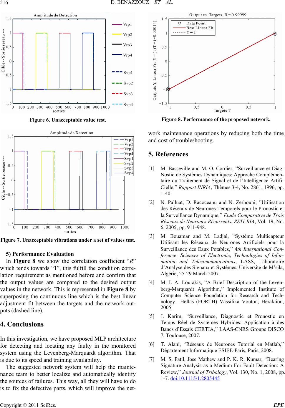

D. BENAZZOUZ ET AL.

516

Figure 8. Performance of the proposed network.

Figure 6. Unacceptable value test.

work maintenance operations by reducing both the time

and cost of troubleshooting.

5. References

[1] M. Basseville and M.-O. Cordier, “Surveillance et Diag-

Nostic de Systèmes Dynamiques: Approche Complémen-

taire du Traitement de Signal et de l’Intelligence Artifi-

Cielle,” Rapport INRIA, Thèmes 3-4, No. 2861, 1996, pp.

1-40.

[2] N. Palluat, D. Racoceanu and N. Zerhouni, “Utilisation

des Réseaux de Neurones Temporels pour le Pronostic et

la Surveillance Dynamique,” Etude Comparative de Trois

Réseaux de Neurones Récurrents, RSTI-RIA, Vol. 19, No.

6, 2005, pp. 911-948.

[3] M. Bouamar and M. Ladjal, “Système Multicapteur

Utilisant les Réseaux de Neurones Artificiels pour la

Surveillance des Eaux Potables,” 4th International Con-

ference: Sciences of Electronic, Technologies of Infor-

mation and Telecommunications, LASS, Laboratoire

d’Analyse des Signaux et Systèmes, Université de M’sila,

Algérie, 25-29 March 2007.

Figure 7. Unacceptable vibrations under a set of values test.

5) Performance Evaluation

In Figure 8 we show the correlation coefficient “R”

which tends towards “1”, this fulfill the condition corre-

lation requirement as mentioned before and confirm that

the output values are compared to the desired output

values in the network. This is represented in Figure 8 by

superposing the continuous line which is the best linear

adjustment fit between the targets and the network out-

puts (dashed line).

[4] M. I. A. Lourakis, “A Brief Description of the Leven-

berg-Marquardt Algorithm,” Implemented Institute of

Computer Science Foundation for Research and Tech-

nology—Hellas (FORTH) Vassilika Vouton, Heraklion,

2005.

[5] J. Karim, “Surveillance, Diagnostic et Pronostic en

Temps Réel de Systèmes Hybrides: Application à des

Bancs d’Essais CERTIA,” LAAS-CNRS Groupe DISCO

7, Toulouse, 2007.

4. Conclusions

In this investigation, we have proposed MLP architecture

for detecting and locating any faulty in the monitored

system using the Levenberg-Marquardt algorithm. That

is due to its speed and training availability.

[6] T. Alani, “Réseaux de Neurones Tutorial en Matlab,”

Département Informatique ESIEE-Paris, Paris, 2008.

[7] M. S. Patil, Jose Mathew and P. K. R. Kumar, “Bearing

Signature Analysis as a Medium For Fault Detection: A

Review,” Journal of Tribology, Vol. 130, No. 1, 2008, pp.

1-7. doi:10.1115/1.2805445

The suggested network system will help the mainte-

nance team to better localize and automatically identify

the sources of failures. This way, all they will have to do

is to fix the defective parts, which will improve the net-