Exploring the Priced Factors in ICAPM in Japan

doi:10.4236/me.2011.24078

Paper Menu >>

Journal Menu >>

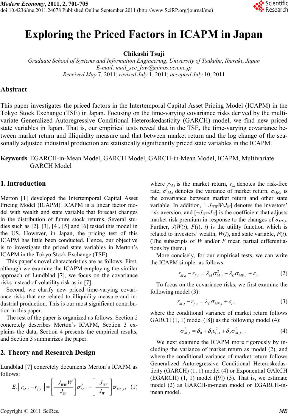Modern Economy, 2011, 2, 701-705

doi:10.4236/me.2011.24078 Published Online September 2011 (http://www.SciRP.org/journal/me)

Exploring the Priced Factors in ICAPM in Japan

Chikashi Tsuji

Graduate School of Systems and Information Engineering, University of Tsukuba, Ibaraki, Japan

E-mail: [email protected]

Received May 7, 2011; revised July 1, 2011; accepted July 10, 2011

Abstract

This paper investigates the priced factors in the Intertemporal Capital Asset Pricing Model (ICAPM) in the

Tokyo Stock Exchange (TSE) in Japan. Focusing on the time-varying covariance risks derived by the multi-

variate Generalized Autoregressive Conditional Heteroskedasticity (GARCH) model, we find new priced

state variables in Japan. That is, our empirical tests reveal that in the TSE, the time-varying covariance be-

tween market return and illiquidity measure and that between market return and the log change of the sea-

sonally adjusted industrial production are statistically significantly priced state variables in the ICAPM.

Keywords: EGARCH-in-Mean Model, GARCH Model, GARCH-in-Mean Model, ICAPM, Multivariate

GARCH Model

1. Introduction

Merton [1] developed the Intertemporal Capital Asset

Pricing Model (ICAPM). ICAPM is a linear factor mo-

del with wealth and state variable that forecast changes

in the distribution of future stock returns. Several stu-

dies such as [2], [3], [4], [5] and [6] tested this model in

the US. However, in Japan, the pricing test of this

ICAPM has little been conducted. Hence, our objective

is to investigate the priced state variables in Merton’s

ICAPM in the Tokyo Stock Exchange (TSE).

This paper’s novel characteristics are as follows. First,

although we examine the ICAPM employing the similar

approach of Lundblad [7], we focus on the covariance

risks instead of volatility risk as in [7].

Second, we clarify new priced time-varying covari-

ance risks that are related to illiquidity measure and in-

dustrial production. This is our most significant contribu-

tion in this paper.

The rest of the paper is organized as follows. Section 2

concretely describes Merton’s ICAPM, Section 3 ex-

plains the data, Section 4 presents the empirical results,

and Section 5 summarizes the paper.

2. Theory and Research Design

Lundblad [7] concretely documents Merton’s ICAPM as

follows:

,,, ,

WW WF

tMt ftMtMFt

JW J

Er rJJ









 







(1)

where rM,t is the market return, rf,t denotes the risk-free

rate, σ2

M,t denotes the variance of market return, σMF,t is

the covariance between market return and other state

variable. In addition, [−JWWW/JW] denotes the investors’

risk aversion, and [−JWF/JW] is the coefficient that adjusts

market risk premium in response to the changes of σMF,t.

Further, J(W(t), F(t), t) is the utility function which is

related to investors’ wealth, W(t), and state variable, F(t).

(The subscripts of W and/or F mean partial differentia-

tions by them.)

More concisely, for our empirical tests, we can write

the ICAPM simpler as follows:

,, , ,.

tftMMtCMFtt



 



 (2)

To focus on the covariance risks, we first examine the

following model (3):

,, ,,

tft CMFtt







 (3)

where the conditional variance of market return follows

GARCH (1, 1) model ([8]) as the following model (4):

,0112,1

MttMt





  (4)

We next examine the ICAPM more rigorously by in-

cluding the variance of market return as model (2), and

where the conditional variance of market return follows

Generalized Autoregressive Conditional Heteroskedas-

ticity (GARCH) (1, 1) model (4) or Exponential GARCH

(EGARCH) (1, 1) model ([9]) (5). That is, we estimate

model (2) as GARCH-in-mean model or EGARCH-in-

mean model.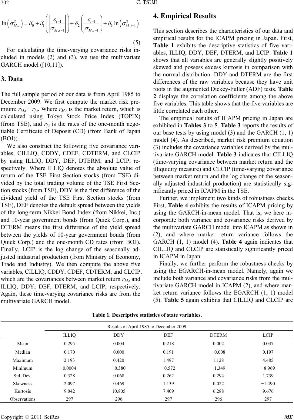

C. TSUJI

702

 

,0123 ,1

,1 ,1

ln ln

Mt Mt



 



 





 





(5)

For calculating the time-varying covariance risks in-

cluded in models (2) and (3), we use the multivariate

GARCH model ([10,11]).

3. Data

The full sample period of our data is from April 1985 to

December 2009. We first compute the market risk pre-

mium: rM,t − rf,t. Where rM,t is the market return, which is

calculated using Tokyo Stock Price Index (TOPIX)

(from TSE), and rf,t is the rates of the one-month nego-

tiable Certificate of Deposit (CD) (from Bank of Japan

(BOJ)).

We also construct the following five covariance vari-

ables, CILLIQ, CDDY, CDEF, CDTERM, and CLCIP

by using ILLIQ, DDY, DEF, DTERM, and LCIP, re-

spectively. Where ILLIQ denotes the absolute value of

return of the TSE First Section stocks (from TSE) di-

vided by the total trading volume of the TSE First Sec-

tion stocks (from TSE), DDY is the first difference of the

dividend yield of the TSE First Section stocks (from

TSE), DEF denotes the default spread between the yields

of the long-term Nikkei Bond Index (from Nikkei, Inc.)

and 10-year government bonds (from Quick Corp.), and

DTERM means the first difference of the yield spread

between the yields of 10-year government bonds (from

Quick Corp.) and the one-month CD rates (from BOJ).

Finally, LCIP is the log change of the seasonally ad-

justed industrial production (from Ministry of Economy,

Trade and Industry). We then compute the above five

variables, CILLIQ, CDDY, CDEF, CDTERM, and CLCIP,

which are the covariances between market return rM,t and

ILLIQ, DDY, DEF, DTERM, and LCIP, respectively.

Again, these time-varying covariance risks are from the

multivariate GARCH model.

4. Empirical Results

This section describes the characteristics of our data and

empirical results for the ICAPM pricing in Japan. First,

Table 1 exhibits the descriptive statistics of five vari-

ables, ILLIQ, DDY, DEF, DTERM, and LCIP. Table 1

shows that all variables are generally slightly positively

skewed and possess excess kurtosis in comparison with

the normal distribution. DDY and DTERM are the first

differences of the raw variables because they have unit

roots in the augmented Dickey-Fuller (ADF) tests. Table

2 displays the correlation coefficients among the above

five variables. This table shows that the five variables are

little correlated each other.

The empirical results of ICAPM pricing in Japan are

exhibited in Tables 3 to 5. Table 3 reports the results of

our base tests by using model (3) and the GARCH (1, 1)

model (4). As described, market risk premium equation

(3) includes the covariance variables derived by the mul-

tivariate GARCH model. Table 3 indicates that CILLIQ

(time-varying covariance between market return and the

illiquidity measure) and CLCIP (time-varying covariance

between market return and the log change of the season-

ally adjusted industrial production) are statistically sig-

nificantly priced in ICAPM in the TSE.

Further, we implement two kinds of robustness checks.

First, Table 4 exhibits the results of ICAPM pricing by

using the GARCH-in-mean model. That is, we here in-

corporate both variance and covariance risks derived by

the multivariate GARCH model into ICAPM as shown in

(2), and where market return variance follows the

GARCH (1, 1) model (4). Table 4 again indicates that

CILLIQ and CLCIP are statistically significantly priced

in ICAPM in Japan.

Finally, we further perform the robustness checks by

using the EGARCH-in-mean model. Namely, again we

include both variance and covariance risks from the mul-

tivariate GARCH model in ICAPM (2), and where mar-

ket return variance follows the EGARCH (1, 1) model

(5). Table 5 again exhibits that CILLIQ and CLCIP are

Table 1. Descriptive statistics of state variables.

Results of April 1985 to December 2009

ILLIQ DDY DEF DTERM LCIP

Mean 0.295 0.004 0.218 0.002 0.047

Median 0.170 0.000 0.191 −0.008 0.197

Maximum 2.193 0.420 1.497 1.128 4.485

Minimum 0.0004 −0.380 −0.572 −1.349 −8.969

Std. Dev. 0.328 0.068 0.262 0.294 1.739

Skewness 2.097 0.469 1.139 0.022 −1.490

Kurtosis 9.042 10.805 7.409 6.288 9.676

Observations 297 296 297 296 297

C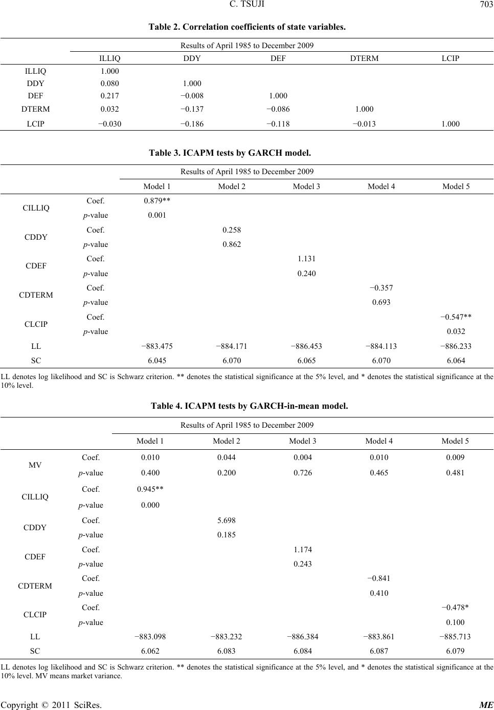. TSUJI703

Table 2. Correlation coefficients of state variables.

Results of April 1985 to December 2009

ILLIQ DDY DEF DTERM LCIP

ILLIQ 1.000

DDY 0.080 1.000

DEF 0.217 −0.008 1.000

DTERM 0.032 −0.137 −0.086 1.000

LCIP −0.030 −0.186 −0.118 −0.013 1.000

Table 3. ICAPM tests by GARCH model.

Results of April 1985 to December 2009

Model 1 Model 2 Model 3 Model 4 Model 5

Coef. 0.879**

CILLIQ p-value 0.001

Coef. 0.258

CDDY p-value 0.862

Coef. 1.131

CDEF p-value 0.240

Coef. −0.357

CDTERM p-value 0.693

Coef. −0.547**

CLCIP p-value 0.032

LL −883.475 −884.171 −886.453 −884.113 −886.233

SC 6.045 6.070 6.065 6.070 6.064

LL denotes log likelihood and SC is Schwarz criterion. ** denotes the statistical significance at the 5% level, and * denotes the statistical significance at the

10% level.

Table 4. ICAPM tests by GARCH-in-mean model.

Results of April 1985 to December 2009

Model 1 Model 2 Model 3 Model 4 Model 5

Coef. 0.010 0.044 0.004 0.010 0.009

p-value 0.400 0.200 0.726 0.465 0.481

Coef. 0.945**

CILLIQ

p-value 0.000

Coef. 5.698

CDDY p-value 0.185

Coef. 1.174

CDEF p-value 0.243

Coef. −0.841

CDTERM p-value 0.410

Coef. −0.478*

CLCIP p-value 0.100

LL −883.098 −883.232 −886.384 −883.861 −885.713

SC 6.062 6.083 6.084 6.087 6.079

LL denotes log likelihood and SC is Schwarz criterion. ** denotes the statistical significance at the 5% level, and * denotes the statistical significance at the

10% level. MV means market variance.

C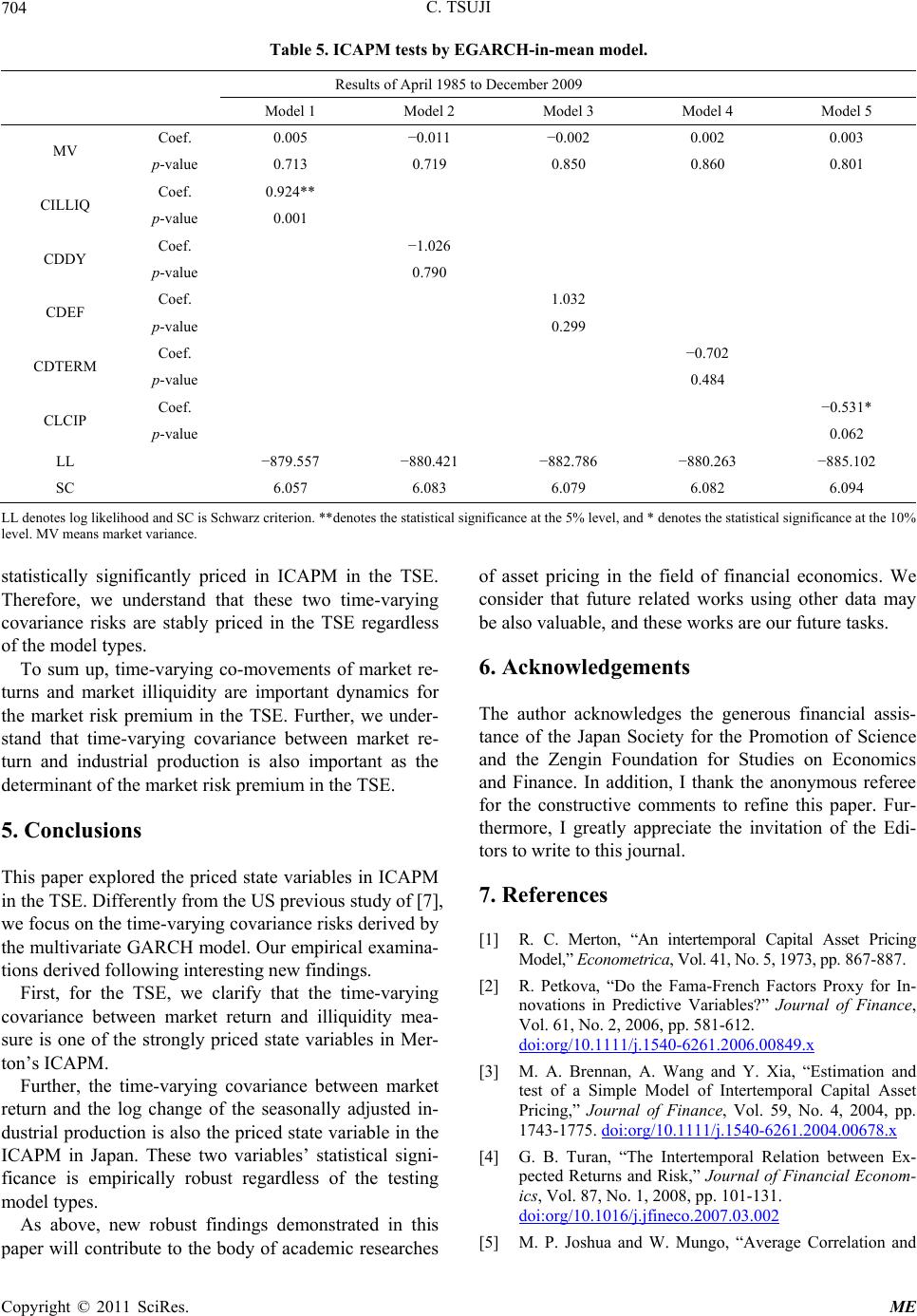. TSUJI

704

Table 5. ICAPM tests by EGARCH-in-mean model.

Results of April 1985 to December 2009

Model 1 Model 2 Model 3 Model 4 Model 5

Coef. 0.005 −0.011 −0.002 0.002 0.003

MV p-value 0.713 0.719 0.850 0.860 0.801

Coef. 0.924**

CILLIQ p-value 0.001

Coef. −1.026

CDDY p-value 0.790

Coef. 1.032

CDEF p-value 0.299

Coef. −0.702

CDTERM p-value 0.484

Coef. −0.531*

CLCIP p-value 0.062

LL −879.557 −880.421 −882.786 −880.263 −885.102

SC 6.057 6.083 6.079 6.082 6.094

LL denotes log likelihood and SC is Schwarz criterion. **denotes the statistical significance at the 5% level, and * denotes the statistical significance at the 10%

level. MV means market variance.

statistically significantly priced in ICAPM in the TSE.

Therefore, we understand that these two time-varying

covariance risks are stably priced in the TSE regardless

of the model types.

To sum up, time-varying co-movements of market re-

turns and market illiquidity are important dynamics for

the market risk premium in the TSE. Further, we under-

stand that time-varying covariance between market re-

turn and industrial production is also important as the

determinant of the market risk premium in the TSE.

5. Conclusions

This paper explored the priced state variables in ICAPM

in the TSE. Differently from the US previous study of [7],

we focus on the time-varying covariance risks derived by

the multivariate GARCH model. Our empirical examina-

tions derived following interesting new findings.

First, for the TSE, we clarify that the time-varying

covariance between market return and illiquidity mea-

sure is one of the strongly priced state variables in Mer-

ton’s ICAPM.

Further, the time-varying covariance between market

return and the log change of the seasonally adjusted in-

dustrial production is also the priced state variable in the

ICAPM in Japan. These two variables’ statistical signi-

ficance is empirically robust regardless of the testing

model types.

As above, new robust findings demonstrated in this

paper will contribute to the body of academic researches

of asset pricing in the field of financial economics. We

consider that future related works using other data may

be also valuable, and these works are our future tasks.

6. Acknowledgements

The author acknowledges the generous financial assis-

tance of the Japan Society for the Promotion of Science

and the Zengin Foundation for Studies on Economics

and Finance. In addition, I thank the anonymous referee

for the constructive comments to refine this paper. Fur-

thermore, I greatly appreciate the invitation of the Edi-

tors to write to this journal.

7. References

[1] R. C. Merton, “An intertemporal Capital Asset Pricing

Model,” Econometrica, Vol. 41, No. 5, 1973, pp. 867-887.

[2] R. Petkova, “Do the Fama-French Factors Proxy for In-

novations in Predictive Variables?” Journal of Finance,

Vol. 61, No. 2, 2006, pp. 581-612.

doi:org/10.1111/j.1540-6261.2006.00849.x

[3] M. A. Brennan, A. Wang and Y. Xia, “Estimation and

test of a Simple Model of Intertemporal Capital Asset

Pricing,” Journal of Finance, Vol. 59, No. 4, 2004, pp.

1743-1775. doi:org/10.1111/j.1540-6261.2004.00678.x

[4] G. B. Turan, “The Intertemporal Relation between Ex-

pected Returns and Risk,” Journal of Financial Econom-

ics, Vol. 87, No. 1, 2008, pp. 101-131.

doi:org/10.1016/j.jfineco.2007.03.002

[5] M. P. Joshua and W. Mungo, “Average Correlation and

C. TSUJI705

Stock Market Returns,” Journal of Financial Economics,

Vol. 96, No. 3, 2010, pp. 364-380.

doi:org/10.1016/j.jfineco.2010.02.011

[6] Y. Jianfeng and Y. Yu, “Investor Sentiment and the

Mean–Variance Relation,” Journal of Financial Eco-

nomics, Vol. 100, No. 2, 2011, pp. 367-381.

doi:org/10.1016/j.jfineco.2010.10.011

[7] C. Lundblad, “The Risk Return Tradeoff in the Long Run:

1836-2003,” Journal of Financial Economics, Vol. 85,

No. 1, 2007, pp. 123-150.

doi:org/10.1016/j.jfineco.2006.06.003

[8] T. Bollerslev, “Generalized Autoregressive Conditional

Heteroskedasticity,” Journal of Econometrics, Vol. 31,

No. 3, 1986, pp. 307-327.

doi:org/10.1016/0304-4076(86)90063-1

[9] D. B. Nelson, “Conditional Heteroskedasticity in Asset

Returns: A New Approach,” Econometrica, Vol. 59, No.

2, 1991, pp. 347-370.

[10] R. F. Engle and K. F. Kroner, “Multivariate simultaneous

generalized ARCH,” Econometric Theory, Vol. 11, No. 1,

1995, pp. 122-150. doi:org/10.1017/S0266466600009063

[11] K. F. Kroner and V. K. Ng, “Modeling Asymmetric Co-

movement of Assets Returns,” Review of Financial Stud-

ies, Vol. 11, No. 4, 1998, pp. 817-844.

doi:org/10.1093/rfs/11.4.817