Identification and Adaptive Control of Dynamic Nonlinear Systems Using Sigmoid Diagonal Recurrent Neural Network

doi:10.4236/ica.2011.23021

Paper Menu >>

Journal Menu >>

Intelligent Control and Automation, 2011, 2, 176-181

doi:10.4236/ica.2011.23021 Published Online August 2011 (http://www.SciRP.org/journal/ica)

Identification and Adaptive Control of Dynamic Nonlinear

Systems Using Sigmoid Diagonal Recurrent Neural

Network

Tarek Aboueldahab1, Mahumod Fakhreldin2

1Cairo Metro Company, Ministry of Transport, Cairo, Egypt

2Computers and Systems Department, Electronic Research Institute, Cairo, Egypt

E-mail: [email protected], [email protected]

Received April 28, 2011; revised May 12, 2011; accepted May 19, 2011

Abstract

The goal of this paper is to introduce a new neural network architecture called Sigmoid Diagonal Recurrent

Neural Network (SDRNN) to be used in the adaptive control of nonlinear dynamical systems. This is done

by adding a sigmoid weight victor in the hidden layer neurons to adapt of the shape of the sigmoid function

making their outputs not restricted to the sigmoid function output. Also, we introduce a dynamic back

propagation learning algorithm to train the new proposed network parameters. The simulation results showed

that the (SDRNN) is more efficient and accurate than the DRNN in both the identification and adaptive con-

trol of nonlinear dynamical systems.

Keywords: Sigmoid Diagonal Recurrent Neural Networks, Dynamic Back Propagation, Dynamic Nonlinear

Systems, Adaptive Control

1. Introduction

The remarkable learning capability of neural networks is

leading to their wide application in identification and

adaptive control of nonlinear dynamical systems [1,2-5,6]

and the tracking accuracy depends on neural networks

structure, which should be chosen properly [7-13].

Feedforward Neural Network (FNN) [4] is a static

mapping and can not reflect the dynamics of the nonlin-

ear systems without using Tapped Delay Lines (TDL)

[7,9]. Fully connected Recurrent Neural Network (RNN)

[9,14,15] contains interlink between neurons to reflect

this dynamics but it suffers both structure complexity

and the poor performance accuracy [9,15]. Based on Lo-

cally Recurrent Globally Feedforward network architec-

tures (LRGF) many researchers focused in (DRNN)

which doesn't contain interlink between hidden layer

neurons leading to the network structure complexity re-

duction [15,8-10].

However, in all these architectures, the hidden layer

neurons output restricted to the sigmoid function output

which represents a major disadvantage in the network

behavior and significantly reduces its performance accu-

racy. Therefore, a new architecture called Sigmoid Di-

agonal Recurrent Neural Network (SDRNN) based on

the hidden layer sigmoid weight and its associated dy-

namic back propagation learning algorithm is proposed.

Simulation results show that SDRNN is more suited than

the (DRNN) for identification and adaptive control of

nonlinear dynamical systems [9].

This paper is organized as follows: Section II presents

some background concerning application of neural net-

works in adaptive control, Section III introduce the new

architecture and its associated dynamical learning algo-

rithm for adaptation of the sigmoid weight. Simulation

results are shown in Section IV, and finally, conclusion

and future work is shown in Section V.

2. Neural Network in Nonlinear System

Identification and Control

In the identification stage of the adaptive control of

nonlinear dynamical system, a neural network identifier

model for the system to be controlled is developed. Then,

this identifier is used to represent the system while train-

ing the neural network controller weights in the control

T. ABOUELDAHAB ET AL.177

stage [6,8,10,12].

2.1. Identification

If a set of data (measurements) can be carried out on a

nonlinear dynamic system, an identifier could be derived

whose dynamic behavior should be as close as possible

to this system. The identifier model is selected based on

whether all the system states or only its output are meas-

ured [1,3,4,9].

The state space representation of a nonlinear system is

given by the following equation:

 



 







1, and ,



kxkukyk xkuk (1)

where: the input to the system,



uk R





kR

the states of the system,



yk R

R

is the outputs of the

system, the nonlinear mappings functions

and are dynamic and

smooth [4,9].

:

nm n

RR Rp



Usually, all the system states are not measured for

process representation, so the Input/Output representa-

tion which is also called Nonlinear Autoregressive Mov-

ing Average (NARMA) representation given by the fol-

lowing equation is used instead [4,6,9]

 



 



,1,, 1

,,1

yk dykykyk n

ukuk m



 





(2)

where d is the relative degree (or equivalent delay) of the

system and it is assumed that both the order of the sys-

tem n and relative degree are specified while the nonlin-

ear function is unknown. ()

In general, any discrete time dynamical nonlinear sys-

tem can be represented using NARMA—Output Error

Model representation shown in Figure 1 and has the fol-

lowing forms:

 









ˆ,1,,

1,,1,,

mmm

ykd ykyk

yknukuk

uk mWk



 

 





(3)

It is crucial to note that, the present identifier output



k represented by the nonlinear mapping function

()



 is a dynamic mapping function because it depends

on its past outputs. Thus, the feed forward neural net-

work can not be used to represent this mapping function

and the recurrent neural network which is a dynamic non

linear mapping is used instead. [9].

2.2. Control

According to both inverse function theorem and implicit



()





ym(k)

u(k)

-1 Z-1 Z-1

Z-1 Z-1 Z-1

Figure 1. NARMA—output error model.

function theorem [4,5,9], if the state vector





kof the

nonlinear system given by equation (1) is accessible,

then the system output





kcan make exact tracking of

a general output





 using a control low given by

the following equation







 





,ukxkyk d





 (4)

If the nonlinear dynamical system given by equations

(1-2) is observable, then the control law can also

be represented in terms of its past values:











1, 1,ukuk m



 as well as previous dynamic

system outputs





,, 1yk n



yk  and





ykd











represents the information that is needed at

the instant to implement the control law (i.e.,









rk ykd





 ) so the above equation can be re-

written as follows [1,3-5,9]:











 







,1,, 1,

(),(1),,1,

ukykykyk n

uk ukukmrk















(5)

As this control law is represented by the nonlinear

dynamical mapping function





, so a neural network

controller model represented by the nonlinear dynamical

mapping function









can be used to achieve the con-

trol law and can be written as:





 



,1,, 1,,

1,,1,,

ukykykyk nuk

ukukmrk Wk















(6)

and







is the set of parameters of the neural network

controller.

As the neural network controller output





ukdepends

on its past outputs, thus, the recurrent neural network

controller is used to evaluate the controller parameters [9].

The structure of the closed loop nonlinear predictive

controller consisting of the nonlinear system, the nonlin-

ear identifier and the nonlinear controller is shown in

Figure 2.

3. The Sigmoid Diagonal Recurrent Neural

Network(SDRNN)

In this section, our proposed architecture and its associ-

T. ABOUELDAHAB ET AL.

178

Figure 2. The structure of the closed loop nonlinear predic-

tive controller.

ated modified dynamic back propagation learning algo-

rithm to learn the new added sigmoid weight vector are

presented

Define the following to obtain the mathematical model

of the proposed neural network architecture:

i,h,o are the number of neurons in input, hidden,

and output layers respectively.

n nn

W is the input weight matrix connecting between

input layer and the hidden layer, ,

are the sig-

moid weight vector and the diagonal weight vector of the

hidden layer, and is the output weight matrix con-

necting between hidden layer and the output layer

Assume, at sample k, the input to the input neu-

ron in the input layer is



k, so the output of the neu-

ral network can be calculated as follows:

The net input to the sigmoid neuron in the hidden

layer can be calculated as follows

 

jjj iji

inkWHkWIk



 

 (7)

And it’s output can be calculated as









fHinkW

Hk W



 (8)

The output of the neuron in the output layer can

be written as follows

 

mjm

YkWHk





j

(9)

For the standard Diagonal Recurrent Neural Network,

the sigmoid weight vector is set to be one and

for the normal Feed Forward Neural Networks the di-

agonal vector







Wk is set to be zero.

Learning Algorithm

Given the structure of the network described by Equa-

tions (7)-(9) and applying the gradient descent method [9,

16] to update the network weights the partial derivatives

of the neural network predictor output with re-

spect to network weights are given by







jk



 (10a)





Yk

SS



 (10b)







jm j

k (10c)







jm ij

k (10d)

where:













jj jj

fHin





()



k WfHinkW

kWW







 

()1 1

jj j P

PkH kWk



















()

j i

k I



(11a)



() ()

ijj ij

QkkW QkC







 









 (11b)

and

 



00,



jij

fHinkW

Hin k





 





From Equation (9), the partial derivatives of the neural

network predictor output represented by the

nonlinear mapping function with respect

to output weight matrix











W is:





k



which lead to (10a).

Also, the partial derivative with respect to sigmoid

weight vector

W is











Yk

And from Equations (7) and (8),

T. ABOUELDAHAB ET AL.179



() 1

ss s

jj j

fHinkW

WW W

fHinkWWW



















 



jj jj

ss ss

jj jj

fHink WfHink W

WW WW



 



 













which lead to (10b).

From Equation (9), the partial derivatives with respect

to diagonal weight vector

W is







mOO

jmjm j

Yk WW



 



and from Equation (8)

 





Ds D

jj j

fHinkW

WW W















Ds D

jj j

fHinkW

kHin

Hin k

WW W





 





and from Equation (7)

  

Hin kHk

Hk W









which leads to (10c), (11a).

Also, the partial derivative with respect to input

weight matrix

W is

()

() ()

mjmjm ij

ij ij

Yk WW



 



and from Equation (8)

 





Is I

ij jij

fHinkW

WW W















Is I

ij jij

fHinkWj

Hin kWW W





 



Hink



and from Equation (7)

  

ij ij

Hin kHk

Ik W









which leads to (10d), (11b).

The full proof of this lemma is given in details in ref-

erence number [9].

4. Results and Discussion

In this section, extensive experimentation is carried out

in an attempt to demonstrate the performance of the

SDRNN architecture and compare it to the DRNN archi-

tecture in nonlinear system identification and in adaptive

control of nonlinear dynamical systems. As a measure to

test the performance, we use the Mean Square Error

(MSE) criteria between the actual nonlinear system out-

put and the neural network output [8-10]. It is worth

mentioning that in our proposed network, there is no

need to use momentum term or learning rate adaptation

[8, 10] because the training is done using the adaptation

of the sigmoid function shape leading to reduction of the

learning algorithm complexity [9].

Example 1: (N o nl i ne a r s y stem identificati o n )

A benchmark problem is employed, the identification

of a dynamical system. The example is taken from [7,9],

where the nonlinear system to be identified is governed

by the following difference equation







  



  

121 2

11 2

Yk YkYkukYk

YkYk

Yk Yk













(12)

As it can be seen, the current output of the plant





1Yk



depends on three previous outputs













,1,Yk 2Yk Yk



 and two previous inputs









1k,uk u



. A NARMA-Output Error Model given

by Equation (3) is considered for identification of this

nonlinear dynamical system. The neural network identi-

fier output







is the approximation of the

nonlinear system output





1Yk. Thus the input to the

neural network identifier are the three previous identifier

outputs i.e. (









,Yk



2,1Yk

Yk m) and the two

previous inputs









,1ukuk



and the size of the neu-

ral network identifier is 5-8-1’ (5 input units, 8 hid-

den units, and one output unit).

In order to comply with previous results reported in

the literature, a new training data containing 200 batches

of 900 patterns is generated. For each data batch, the

input





uk is an independent and identically distrib-

uted uniform in the range between



while the

testing data set is composed of 1000 samples with a sig-

nal described by



1, 1



 



sin π25 250

1 250500

()1 500750

0.3sin π250.1sin π32

0.6sin π10 7501000

uk k







 







 



(13)

As a measure to test the identification performance,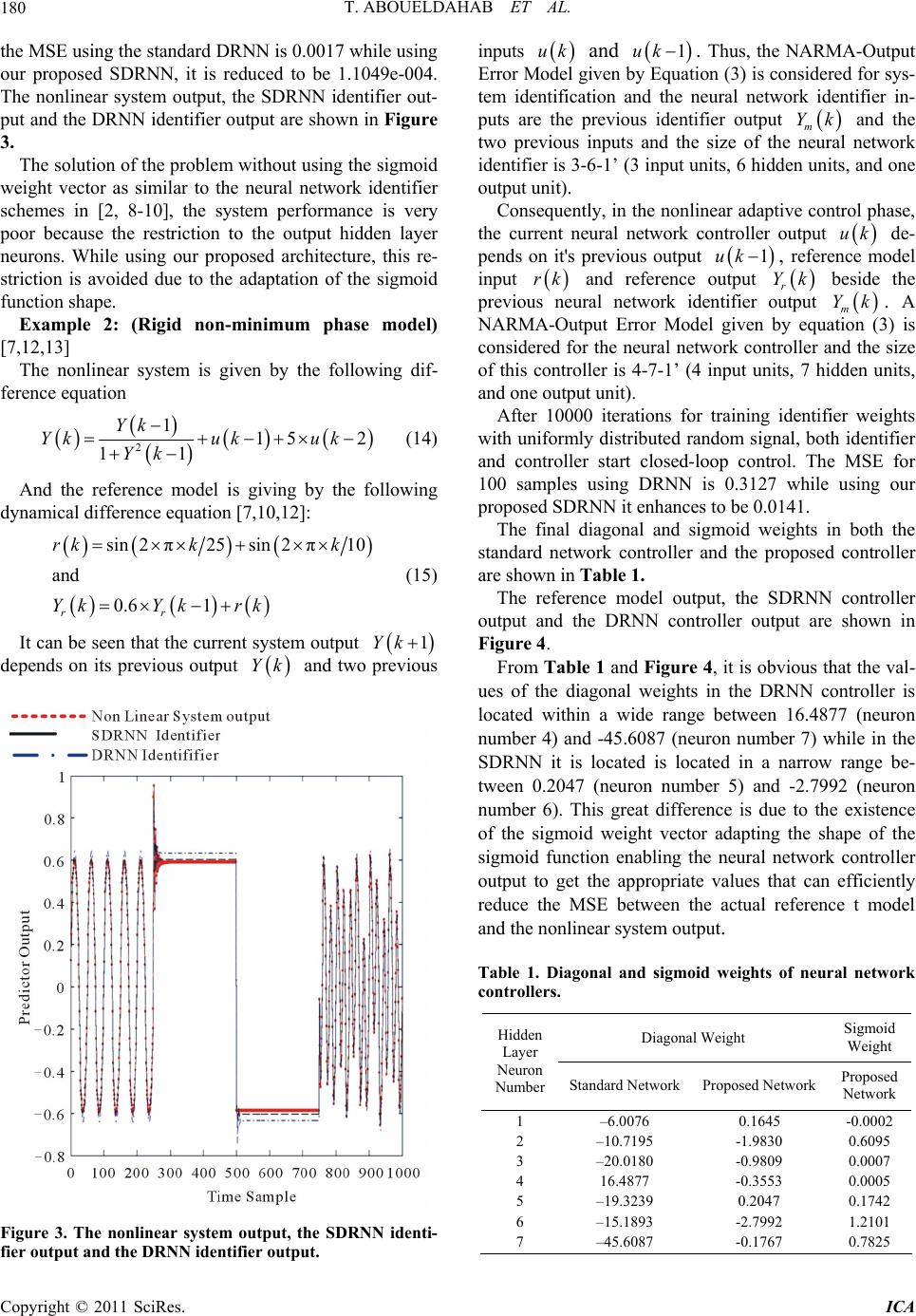

T. ABOUELDAHAB ET AL.

180

the MSE using the standard DRNN is 0.0017 while using

our proposed SDRNN, it is reduced to be 1.1049e-004.

The nonlinear system output, the SDRNN identifier out-

put and the DRNN identifier output are shown in Figure

The solution of the problem without using the sigmoid

weight vector as similar to the neural network identifier

schemes in [2, 8-10], the system performance is very

poor because the restriction to the output hidden layer

neurons. While using our proposed architecture, this re-

striction is avoided due to the adaptation of the sigmoid

function shape.

Example 2: (Rigid non-minimum phase model)

[7,12,13]

The nonlinear system is given by the following dif-

ference equation

 



 

115 2

Ykuk uk











(14)

And the reference model is giving by the following

dynamical difference equation [7,10,12]:

 



sin 2π25sin2π10

and

0.6 1

rk kk

YkYk rk



 

(15)

It can be seen that the current system output





1Yk



depends on its previous output and two previous



Figure 3. The nonlinear system output, the SDRNN identi-

fier output and the DRNN identifier output.

inputs





uk and





1uk



. Thus, the NARMA-Output

Error Model given by Equation (3) is considered for sys-

tem identification and the neural network identifier in-

puts are the previous identifier output and the

two previous inputs and the size of the neural network

identifier is 3-6-1’ (3 input units, 6 hidden units, and one

output unit).



Consequently, in the nonlinear adaptive control phase,

the current neural network controller output





uk de-

pends on it's previous output , reference model

input



1uk







rk and reference output beside the

previous neural network identifier output







Yk. A

NARMA-Output Error Model given by equation (3) is

considered for the neural network controller and the size

of this controller is 4-7-1’ (4 input units, 7 hidden units,

and one output unit).

After 10000 iterations for training identifier weights

with uniformly distributed random signal, both identifier

and controller start closed-loop control. The MSE for

100 samples using DRNN is 0.3127 while using our

proposed SDRNN it enhances to be 0.0141.

The final diagonal and sigmoid weights in both the

standard network controller and the proposed controller

are shown in Table 1.

The reference model output, the SDRNN controller

output and the DRNN controller output are shown in

Figure 4.

From Ta ble 1 and Figure 4, it is obvious that the val-

ues of the diagonal weights in the DRNN controller is

located within a wide range between 16.4877 (neuron

number 4) and -45.6087 (neuron number 7) while in the

SDRNN it is located is located in a narrow range be-

tween 0.2047 (neuron number 5) and -2.7992 (neuron

number 6). This great difference is due to the existence

of the sigmoid weight vector adapting the shape of the

sigmoid function enabling the neural network controller

output to get the appropriate values that can efficiently

reduce the MSE between the actual reference t model

and the nonlinear system output.

Table 1. Diagonal and sigmoid weights of neural network

controllers.

Diagonal Weight Sigmoid

Weight

Hidden

Layer

Neuron

Number Standard NetworkProposed Network Proposed

Network

–6.0076

–10.7195

–20.0180

16.4877

–19.3239

–15.1893

0.1645

–45.6087

-1.9830

-0.9809

-0.3553

0.2047

-2.7992

-0.0002

0.6095

0.0007

0.0005

0.1742

1.2101

-0.1767 0.7825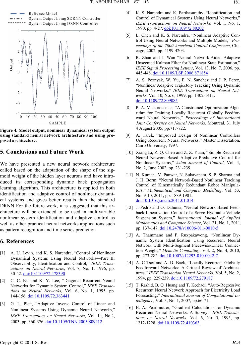

T. ABOUELDAHAB ET AL.

181

[4] K. S. Narendra and K. Parthasarathy, “Identification and

Control of Dynamical Systems Using Neural Networks,”

IEEE Transactions on Neural Networks, Vol. 1, No. 1,

1990, pp. 4-27. doi:10.1109/72.80202

[5] L. Chen and K. S. Narendra, “Nonlinear Adaptive Con-

trol Using Neural Networks and Multiple Models,” Pro-

ceedings of the 2000 American Control Conference, Chi-

cago, 2002, pp. 4199-4203.

[6] R. Zhan and J. Wan “Neural Network-Aided Adaptive

Unscented Kalman Filter for Nonlinear State Estimation,”

IEEE Signal Processing Letters, Vol. 13, No. 7, 2006, pp.

445-448. doi:10.1109/LSP.2006.871854

[7] A. S. Poznyak, W. Yu, E. N. Sanchez and J. P. Perez,

“Nonlinear Adaptive Trajectory Tracking Using Dynamic

Neural Networks,” IEEE Transactions on Neural Net-

works, Vol. 10, No. 6, 1999, pp. 1402-1411.

doi:10.1109/72.809085

[8] P. A. Mastorocostas, “A Constrained Optimization Algo-

rithm for Training Locally Recurrent Globally Feedfor-

ward Neural Networks,” Proceedings of International

Joint Conference on Neural Networks, Montreal, 31 July

4 August 2005, pp.717-722.

Figure 4. Model output, nonlinear dynamical sy stem output

using standard neural network architecture and using pro-

posed architecture. [9] A. Tarek, “Improved Design of Nonlinear Controllers

Using Recurrent Neural Networks,” Master Dissertation,

Cairo University, 1997.

5. Conclusions and Future Work [10] Xiang Li, Z. Q. Chen and Z. Z. Yuan, “Simple Recurrent

Neural Network-Based Adaptive Predictive Control for

Nonilnear Systems,” Asian Journal of Control, Vol. 4,

No. 2, June 2002, pp. 231-239.

We have presented a new neural network architecture

called based on the adaptation of the shape of the sig-

moid weight of the hidden layer neurons and have intro-

duced its corresponding dynamic back propagation

learning algorithm. This architecture is applied in both

identification and adaptive control of nonlinear dynami-

cal systems and gives better results than the standard

DRNN For the future work, it is suggested that this ar-

chitecture will be extended to be used in multivariable

nonlinear system identification and adaptive control as

well as other practical neural networks applications such

as pattern recognition and time series prediction

[11] N. Kumar , V. Panwar, N. Sukavanam, S. P. Sharma and

J. H. Borm, “Neural Network-Based Nonlinear Tracking

Control of Kinematically Redundant Robot Manipula-

tors,” Mathematical and Computer Modelling, Vol. 53,

No. 9-10, 2011, pp. 1889-1901.

doi:10.1016/j.mcm.2011.01.014

[12] J. Pedro and O. Dahunsi, “Neural Network Based Feed-

back Linearization Control of a Servo-Hydraulic Vehicle

Suspension System,” International Journal of Applied

Mathematics and Computer Science, Vol. 21, No. 1, 2011,

pp. 137-147. doi:10.2478/v10006-011-0010-5

[13] A. Thammano and P. Ruxpakawong, “Nonlinear Dy-

namic System Identification Using Recurrent Neural

Network with Multi-Segment Piecewise-Linear Connec-

tion Weight,” Memetic Computing, Vol. 2, No. 4, 2010,

pp. 273-282. doi:10.1007/s12293-010-0042-7

6. References

[1] A. U. Levin, and K. S. Narendra, “Control of Nonlinear

Dynamical Systems Using Neural Networks—Part II:

Observability, Identification and Control,” IEEE Trans-

actions on Neural Networks, Vol. 7, No. 1, 1996, pp.

30-42. doi:10.1109/72.478390

[14] A. C Tsoi and A. D. Back, “Locally Recurrent Globally

Feedforward Networks: A Critical Review of Architec-

tures,” IEEE Transaction Neural Networks, Vol. 5, No. 2,

1994, pp. 229-239. doi:10.1109/72.279187

[2] C. C. Ku and K. Y. Lee, “Diagonal Recurrent Neural

Networks for Dynamic System Control,” IEEE Transac-

tions on Neural Networks, Vol. 6, No. 1, 1995, pp.

144-156. doi:10.1109/72.363441

[15] T. Rashid, B. Q. Huang and T. Kechadi, “Auto-Regressive

Recurrent Neural Network Approach for Electricity Load

Forecasting,” International Journal of Computational In-

telligence, Vol. 3, No. 1, 2007, pp.66-71.

[3] G. L. Plett, “Adaptive Inverse Control of Linear and

Nonlinear Systems Using Dynamic Neural Networks,”

IEEE Transactions on Neural Networks, Vol. 14, No.2,

2003, pp. 360-376. doi:10.1109/TNN.2003.809412

[16] B. A. Pearlmutter, “Gradient Calculations for Dynamic

Recurrent Neural Networks: A Survey,” IEEE Transac-

tions on Neural Networks, Vol. 6, No. 5, 1995, pp.

1212-1228. doi:10.1109/72.410363