

Paper Menu >>
Journal Menu >>
 Applied Mathematics, 2011, 2, 987-992 doi:10.4236/am.2011.28136 Published Online August 2011 (http://www.SciRP.org/journal/am) Copyright © 2011 SciRes. AM A New Analytical Approach for Solving Nonlinear Boundary Value Problems in Finite Domains Jafar Biazar1, Behzad Ghanbari2* 1Department of Applied Mathematics, Faculty of Mathematical Sciences, University of Guilan, Rasht, Iran 2Department of Mat hem at i cs, Kermanshah University of Technology, Kermanshah, Iran E-mail: [email protected] Received November 4, 2010; revised May 25, 2011; accepted July 4, 2011 Abstract Based on the homotopy analysis method (HAM), we propose an analytical approach for solving the follow- ing type of nonlinear boundary value problems in finite domain. In framework of HAM a convenient way to adjust and control the convergence region and rate of convergence of the obtained series solutions, by defin- ing the so-called control parameter , is provided. This paper aims to propose an efficient way of finding the proper values of . Such values of parameter can be determined at the any order of approximations of HAM series solutions by solving of a nonlinear polynomial equation. Some examples of nonlinear initial value problems in finite domain are used to illustrate the validity of the proposed approach. Numerical re- sults confirm that obtained series solutions agree very well with the exact solutions. Keywords: Homotopy Analysis Method, Boundary Value Problems, Finite Domain 1. Introduction In this work, we consider the following typ e of nonlinear boundary value problems in a finite domain (as consid- ered in [1]): ()( 1) ,, ,,, nn uxfxuu uaxb 2 2 (1) subject to th e two-point boundary conditions () 01 (2) 01 ,,, ,() ,, rr nr nr uau aua ub ubub (2) where is an integer. 0rn Also f is a polynomial in and (1) ,,, n, x uxu xux 01 01 2 ,,,,,,, rnr are real constants. Since, such type of boundary value problems arise in the mathematical modeling of the viscoelastic flows and other branches of mathematical, physical and engineer- ing sciences, the approximate solutions of these prob- lems are of great importance. See [2-4] and the refer- ences therein. Some numerical and analytical methods such as shooting method [5], Finite-element method [6], sinc- Galerkin method [7], finite-difference method [8], Ado- mian technique [9], variational iteration method (VIM) [10], homotopy perturbation method (HPM) [11], analy- sis method (HAM) [12], have been studied for obtaining approximate solutions to boundary value problems. The homotopy analysis method [13-17] is a general analytic approach to get series solutions of various types of nonlinear equations, including ordinary differential equations, partial differential equations, differential-in- tegral equations, differential-difference equation, and coupled equations of them. Unlike perturbation methods, the HAM is independent of small/large physical parame- ters, and thus is valid no matter whether a nonlinear problem contains small/large physical parameters or not. More importantly, different from all perturbation and traditional non-perturbation methods, the HAM provides us a simple way to ensure the convergence of solution series, and therefore, the HAM is valid even for strongly nonlinear problems. Besides, different from all perturba- tion and previous non-perturbation methods, the HAM provides us with great freedom to choose proper base functions to approximate a nonlinear problem. These advantages make the method to be a powerful and flexible tool in mathematics and engineering, which can be readily distinguished from existing numerically and analytically methods. Up to now, this method has been successfully applying this method to various nonlinear problems in science and  J. BIAZAR ET AL. 988 ; engineering. A systematic description of the method and its applications are found in [15]. This paper is arranged in the following manner. In Section 2, the HAM is applied to solve the problem of nonlinear boundary value problems. In Section 3, the basic idea of the present approach is described. Further- more, some numerical examples are presented in Section 4. Finally, conclusions are drawn in Section 5. 2. The Implement of HAM to BVPs In order to obtain a convergent series solution to the nonlinear problem (1, 2), we first construct the zeroth order deformation equation 0 1;pLxpu xpNxp (3) where is an embedding parameter, [0,1]p0 is a convergence-control parameter, and ; x p is an unknown function, respectively. According to (1), the auxiliary linear operator is given by L ; ;n n x p Lxp x (4) and the nonlinear operator is given by N 1 1 ;,,, n nn Nxp fxx xx , n (5) From (3), when and , 0p1p 0 ;0 x ux and ;1 x ux both hold. Therefore, as increases from 0 to 1, the p solution ; x p varies from the initial guess 0 uxto the solution ux. Expanding ; x p in Taylor series with respect to, one has p 1 ;;0 i i i x px ux p (6) where 0 ; 1 ! m mm p xp ux mp (7) Assuming that the series (6) is convergent at 1p , The solution series 01 ;1 i i uxxuxu x (8) must be one of the solutions of the original problem (1, 2), as proved by Liao in [15]. Our next goal is to determine the higher order terms (1 m uxm). Define the vector 01 ,,,uss x uxux ux (9) Differentiating the zeroth order deformation Equation (3) times with respect to , then setting mp0p , finally dividing them by , we obtain the th order deformation equation !mm 1mmmm Lu xuxhRx 1 (10) and its boundary cond itions () 0 r mm m ua uaua (11) (2) 0 nr mm m ub ubub where 1 11 0 ; 1 1! m mm p Nxp Rx mp (12) and 1, 1 0, 1 m m m (13) From (4), th order deformation Equation (10) be- comes m () () 1 nn mmm m uxu xhRx 1 1 (14) In this way, the component solutions of , are not only dependent upon , m um x but also the auxiliary pa- rameter . Thus, the convergence of the series (8) de- pends on the parameter . Finally, theth order approximation to the problem (1, 2) can be generally expres sed by m 01 m m i ux uxux i (15) As we know, to find a proper convergence-control pa- rameter , to get a convergent series solution or to get a faster convergent one, there is a classic way of plotting the so-called ‘‘-curves” or ‘‘curves for convergence- control parameter”. For example, one can consider the convergence of ux and of a nonlinear diffe- ux rential equation 0Nux to find a region say R so that, each gives a convergent series solution of such kind of quantities. R Such a region can be found, although approximately, by plotting the curves of these unknown quantities versus . However, it is a pity that curves for convergence- con- trol parameter (i.e. -curves) give us only a graphically region and cannot tell us which value of R gives the fastest convergent series. Furthermore, recently in Copyright © 2011 SciRes. AM  J. BIAZAR ET AL. 989 [18] a misinterpreted usage of-curves has reported. Although the solution series (15) given by different values in the valid region of converge to the exact solution, the convergence rates of these solution series are usually different. i x 3. Proposed Approach It should be noted that based on the zeroth-order defor- mation Equation (3), th-order HAM ap proximation of the solution , giving by m ux 01 m mi ux uux is also dependent upon the convergence-control parame- ter . For 1 2ba , let ()( 1) ,, 0 mm nn m PNu uf uu ,, u (16) donate the residual error of the governing Equation (12) at the th-order of HAM approximation. m Since is indeed a polynomial equation of order , so at each order of approximation , we can gain the value of by solving only one algebraic equa- tion. 0 m P mm 4. Numerical Examples To demonstrate the efficiency of the proposed approach, we consider several examples. For comparison purpose they were taken from [1,12]. Example 1. Let’s consider the following second order boundary value problem [1]. 33 262,1u xuxuxxx 2 (17) with the boundary conditions 5 12,2 2 uu (18) which has the exact solution in the form of 1 uxx x (19) For the zeroth order deformation Equation (3), the auxiliary linear operator is given by L 2 2 ; ; x p Lxp x and the nonlinear operator is given by N 223 2 ; ;2;6; xp Nxpxp xpx x 2 In view of the boundary conditions (18), the initial guess is determined as 2 057 22 ux xx To obtain higher order terms , the th order deformation Equation (10) and its boundary conditions (11) are calculated: m ux m 11mmm m uxux hRx 10, 20 mm uu where 3 11 1 1 00 621 2() u mm mmm j m mjiji ji R xuxuxx uxuxux In this way, we can calculate (1 m uxm) recur- sively. In this example, from Equation (16) with 10m , the proper value for .obtained as . 0.364 As it can be seen in Table 1 and Figure 1, obtained approximate series solution agrees very well with the exact solution (19). Example 2. As the example, let’s have the following third order boundary value problem [1]. (3)2 10,0 1utututut x (20) with the boundary conditions 001uu u 0 (21) This problem was considered in [9] via the finite dif- ference method. For the zeroth order deformation Equation (3), the auxiliary linear operator is given by L 3 3 ; ; x p Lxp x and the nonlinear operator is given by N Table 1. Absolute errors of different methods in Example 1. x Exact solution Shooting method [5]10th HAM for[1] 0.167 10th HAM for 0.364 1.1x2.00909090.00067230.0001009 4.32e–6 1.3x 2.06923080.00216820.0001164 2.59e–7 1.5x 2.16666670.00330090.0004174 7.44e–6 1.7x2.28823530.00362130.0000210 8.15e–6 1.9x 2.42631580.00218490.0007363 1.80e–5 Copyright © 2011 SciRes. AM  990 J. BIAZAR ET AL. Figure 1. Symbols: 5th-order HAM approximation for 0.364; solid line: exact solution. 32 3 2 ; ;; ;1 2 ; x px Nxp xp x xp x p x In view of the boundary conditions (21), the initial guess is determined as 32 0 uxx x ux . To obtain higher order terms m, the th order deformation Equation (10) and its boundary conditions (11) are calculated: m (3) (3)1 00,00, 1 mmm m mmm uxuxhRx uuu 0 where 1 (3)11 0 1 1 01 um mmmi mi i m j mj m j Rxuxuxu uxu x x ) In this way , can be do ne re cursively . (1 m uxm 0.922 In this case, is obtained by our approach. As shown in Table 2 and Figure 2, approximate series solution using such value of parameter, is in excellent agreement with the numerical solution given by the Runge-Kutta-Fehlberg 4-5 technique. Table 2. Absolute errors of different methods in Example 2. x Exact solution Shooting method [5] 10th HAM for [1] 1.23 10th HAM for 0.922 0.1x 2.0090909 0.0006723 1.46e–6 3.96e–7 0.3x 2.0692308 0.0021682 1.41e–6 3.00e–11 0.5x 2.1666667 0.0033009 1.74e–6 1.19e–8 0.7x 2.2882353 0.0036213 2.00e–6 6.89e–8 0.9x 2.4263158 0.0021849 2.31e–6 1.02e–7 Figure 2. Solid line: 5th-order HAM approximation for 0.32683722 ; symbols: numerical solution. Example 3. As the example, let’s have the following nonlinear fourth-order boundary value problem involving a parameter [12]. c 2 (4)1, 02uxcux x (22) with the boundary conditions 0022uu uu 0 (23) For the zeroth order deformation Equation (3), the auxiliary linear operator is given by L 4 4 ; ; x p Lxp x and the nonlinear operato r is given by N 42 4 ; ;; xp Nxp cxp x 1 In view of the boundary conditions (23), the initial guess is determined as 43 044ux xxx2 To obtain higher order terms , the th order deformation Equation (10) and its boundary conditions (11) are calculated: m ux m (4) (4)1 00, 00,20, 20 mmmm mmmm ux uxhRx uuuu where 1 (4)11 0 1um mmmmi im i Rxuxcuxux In this way (1 m uxm) , can be done recursi vely. Copyright © 2011 SciRes. AM 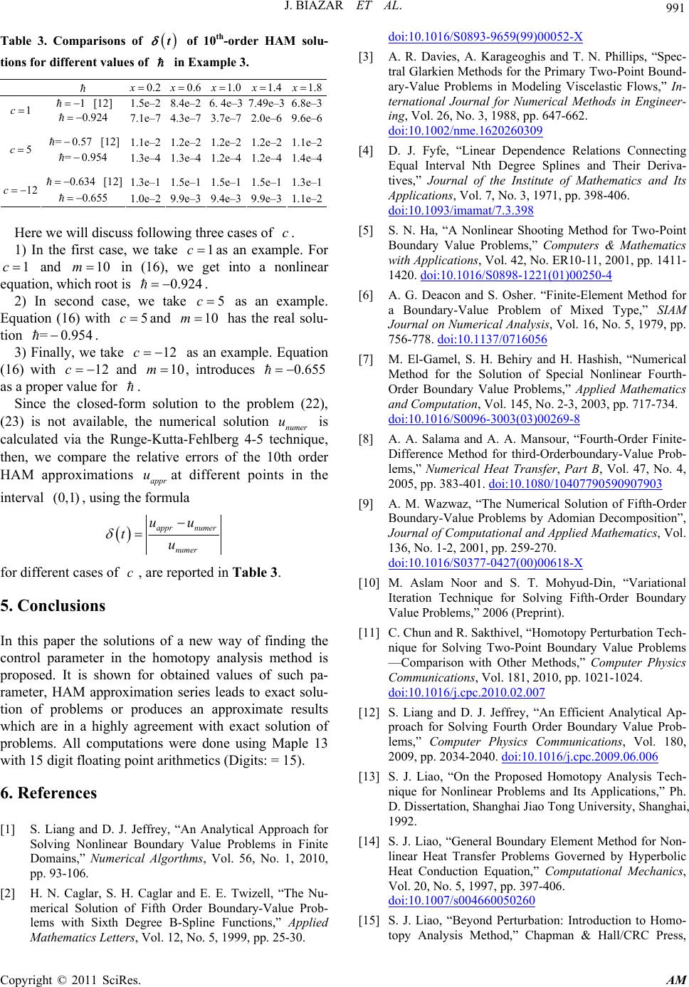 J. BIAZAR ET AL. 991 Table 3. Comparisons of of 10th-order HAM solu- tions for different values of in Example 3. t 0.2x 0.6x 1.0x 1.4x1.8x 1 [12] 1.5e–2 8.4e–2 6. 4e–3 7.49e–36.8e–3 1c 0.924 7.1e–7 4.3e–7 3.7e–7 2.0e–69.6e–6 =0.57 [12] 1.1e–2 1.2e–2 1.2e–2 1.2e–21.1e–2 5c =0.954 1.3e–4 1.3e–4 1.2e–4 1.2e–41.4e–4 0.634 [12] 1.3e–1 1.5e–1 1.5e–1 1.5e–11.3e–1 12c 0.655 1.0e–2 9.9e–3 9.4e–3 9.9e–31.1e–2 Here we will discuss following three cases of . c 1) In the first case, we take as an example. For and in (16), we get into a nonlinear equation, which root is . 1c 0.924 1c10m 2) In second case, we take as an example. Equation (16) with and has the real solu- tion . 5c 105cm =0.954 3) Finally, we take as an example. Equation (16) with and , introduces as a proper value for . 12c 10m 12c 0.655 Since the closed-form solution to the problem (22), (23) is not available, the numerical solution numer is calculated via the Runge-Kutta-Fehlberg 4-5 technique, then, we compare the relative errors of the 10th order u HAM approximations at different points in the appr u interval , using the formula (0,1) appr numer numer uu tu for different cases of , are reported in Table 3. c 5. Conclusions In this paper the solutions of a new way of finding the control parameter in the homotopy analysis method is proposed. It is shown for obtained values of such pa- rameter, HAM approximation series leads to exact solu- tion of problems or produces an approximate results which are in a highly agreement with exact solution of problems. All computations were done using Maple 13 with 15 digit floating point arithmetics (Digits: = 15). 6. References [1] S. Liang and D. J. Jeffrey, “An Analytical Approach for Solving Nonlinear Boundary Value Problems in Finite Domains,” Numerical Algorthms, Vol. 56, No. 1, 2010, pp. 93-106. [2] H. N. Caglar, S. H. Caglar and E. E. Twizell, “The Nu- merical Solution of Fifth Order Boundary-Value Prob- lems with Sixth Degree B-Spline Functions,” Applied Mathematics Letters, Vol. 12, No. 5, 1999, pp. 25-30. doi:10.1016/S0893-9659(99)00052-X [3] A. R. Davies, A. Karageoghis and T. N. Phillips, “Spec- tral Glarkien Methods for the Primary Two-Point Bound- ary-Value Problems in Modeling Viscelastic Flows,” In- ternational Journal for Numerical Methods in Engineer- ing, Vol. 26, No. 3, 1988, pp. 647-662. doi:10.1002/nme.1620260309 [4] D. J. Fyfe, “Linear Dependence Relations Connecting Equal Interval Nth Degree Splines and Their Deriva- tives,” Journal of the Institute of Mathematics and Its Applications, Vol. 7, No. 3, 1971, pp. 398-406. doi:10.1093/imamat/7.3.398 [5] S. N. Ha, “A Nonlinear Shooting Method for Two-Point Boundary Value Problems,” Computers & Mathematics with Applications, Vol. 42, No. ER10-11, 2001, pp. 1411- 1420. doi:10.1016/S0898-1221(01)00250-4 [6] A. G. Deacon and S. Osher. “Finite-Element Method for a Boundary-Value Problem of Mixed Type,” SIAM Journal on Numerical Analysis, Vol. 16, No. 5, 1979, pp. 756-778. doi:10.1137/0716056 [7] M. El-Gamel, S. H. Behiry and H. Hashish, “Numerical Method for the Solution of Special Nonlinear Fourth- Order Boundary Value Problems,” Applied Mathematics and Computation, Vol. 145, No. 2-3, 2003, pp. 717-734. doi:10.1016/S0096-3003(03)00269-8 [8] A. A. Salama and A. A. Mansour, “Fourth-Order Finite- Difference Method for third-Orderboundary-Value Prob- lems,” Numerical Heat Transfer, Part B, Vol. 47, No. 4, 2005, pp. 383-401. doi:10.1080/10407790590907903 [9] A. M. Wazwaz, “The Numerical Solution of Fifth-Order Boundary-Value Problems by Adomian Decomposition”, Journal of Computational and Applied Mathematics, Vol. 136, No. 1-2, 2001, pp. 259-270. doi:10.1016/S0377-0427(00)00618-X [10] M. Aslam Noor and S. T. Mohyud-Din, “Variational Iteration Technique for Solving Fifth-Order Boundary Value Problems,” 2006 (Preprint). [11] C. Chun and R. Sakthivel, “Homotopy Perturbation Tech- nique for Solving Two-Point Boundary Value Problems —Comparison with Other Methods,” Computer Physics Communications, Vol. 181, 2010, pp. 1021-1024. doi:10.1016/j.cpc.2010.02.007 [12] S. Liang and D. J. Jeffrey, “An Efficient Analytical Ap- proach for Solving Fourth Order Boundary Value Prob- lems,” Computer Physics Communications, Vol. 180, 2009, pp. 2034-2040. doi:10.1016/j.cpc.2009.06.006 [13] S. J. Liao, “On the Proposed Homotopy Analysis Tech- nique for Nonlinear Problems and Its Applications,” Ph. D. Dissertation, Shanghai Jiao Tong University, Shanghai, 1992. [14] S. J. Liao, “General Boundary Element Method for Non- linear Heat Transfer Problems Governed by Hyperbolic Heat Conduction Equation,” Computational Mechanics, Vol. 20, No. 5, 1997, pp. 397-406. doi:10.1007/s004660050260 [15] S. J. Liao, “Beyond Perturbation: Introduction to Homo- topy Analysis Method,” Chapman & Hall/CRC Press, Copyright © 2011 SciRes. AM  J. BIAZAR ET AL. Copyright © 2011 SciRes. AM 992 Boca Raton, 2003. doi:10.1201/9780203491164 [16] S. J. Liao, “Numerically Solving Nonlinear Problems by the Homotopy Analysis Method,” Computational Me- chanics, Vol. 20, No. 6, 1997, pp. 530-540. doi:10.1007/s004660050273 [17] S. J. Liao, “Notes on the Homotopy Analysis Method: Some Definitions and Theorems,” Communications in Nonlinear Science and Numerical Simulation, Vol. 14, No. 4, 2009, pp. 983-997. doi:10.1016/j.cnsns.2008.04.013 [18] A. Mehmood, S. Munawar and A. Ali, “Comments to: ‘‘Homotopy Analysis Method for Solving the MHD Flow over a Non-Linear Stretching Sheet,” Communications in Nonlinear Science and Numerical Simulation, Vol. 14, No. 6, 2009, pp. 2653-2663. doi:10.1016/j.cnsns.2009.12.039 |