On chromospheric variations modeling for main-sequence stars of G and K spectral classes

doi:10.4236/ns.2011.38087

Paper Menu >>

Journal Menu >>

Vol.3, No.8, 641-645 (2011) Natural Science

http://dx.doi.org/10.4236/ns.2011.38087

On chromospheric variations modeling for

main-sequence stars of G and K spectral classes

Bruevich Elena Alecsandrovna

Sternberg Astronomical Institute, Moscow, Russia; [email protected]

Received 2 March 2011; revised 13 April 2011; accepted 21 April 2011.

ABSTRACT

We present a method of 13 late-type main-se-

quence stars chromospheric flux observation

data calculations. These Sun-like stars have

well-determined cyclic flux variations similar to

the 11-year solar activity cycle. Our flux predic-

tion is based on chromospheric HK emission

time series measurements from the Mount Wil-

son Observatory and comparable solar data. We

show that solar three-component modeling ex-

plains well the stellar observations. We find that

the 10% - 20% of K-stars disc’s surfaces are

occupied by bright active regions.

Keywords: The Sun; Late-Type Stars;

Chromospheric Emission

1. INTRODUCTION

This paper continues the study of variability among

Sun-like stars. Here the purpose is to obtain the possibil-

ity of modeling the behavior of the star’s chromospheric

emission in future or for periods of time without meas-

urements.

Observations of chromospheric variability requires at

least a decade to reveal variations with timescales to the

11-year solar cycle.

We use the data from the observation program that

was initiated by Wilson who discovered the widespread

occurrence of activity cycles by monitoring Ca II H and

K variations in 91 stars on or near the lower main se-

quence over 12 year. Two sets of measurements (named

“HK-project”) have been combined to make more than

30 years records of stellar chromospheric activity. Wil-

son made observations from 1966 to 1977 at monthly

intervals on 2.5 m telescope at Mount Wilson Observa-

tory. The survey moved in 1977 to 1.5 m telescope with

instrument whose measurements can be compared to

those of Wilson’s system. Some new stars were added to

91 Wilson’s stars to bring the total in the monitoring

program to 111 stars [1,2]. Ca II H (396.8 nm) and K

(393.4 nm) emission is observed in stars with spectral

class later than approximately F2 V, i.e. less massive

than about 1.5

. Areas of concentrated magnetic

fields on the Sun and Sun-like stars emit Ca II H and K

more intensely than areas with less magnetic field pre-

sent. So the contrast of Active Regions (AR) emission

(where the local magnetic fields are more then some

orders higher than average global magnetic field) in

these Ca II lines changes from 1.2 to 1.5 with changing

of chromospheric activity cycle phase.

Comparing of variability of H and K emission in

main-sequence stars should provide important validation

for theories of magnetic activity, as well as place of solar

activity in a general perspective.

The influence of photospheric flux in the total solar or

stars irradiance we can interpretate as the cyclic flux

variations caused by slight imbalance between the flux

deficit produced by dark sunspots and the excess flux

produced by bright faculae. average emission (that varies

with the so-called the 11-year chromospheric cycle).

Besides of such structures as AR in solar and stars

chromosphere there is another regular structure—“chro-

mospheric network” (connecting with the supegranula-

tion). It also varies its own relative brightness with

chromospheric activity cycle.

We can note that the maximum amplitude of photo-

spheric flux variability in the 11-year solar cycle may be

as much as 1% - 3% of the average photospheric flux

level but the maximum amplitude of Ca II chromos-

pheric flux may be as much as 20% of the average level.

These values are our estimations for the maximum am-

plitudes of the 11-year variations of Sun-like stars pho-

tospheric and chromospheric fluxes.

2. THE THREE-COMPONENT MODEL

OF STELLAR CHROMOSPHERIC

EMISSION

The processes in solar atmosphere caused the emis-

sion in different spectral intervals and lines are studied

B. E. Alecsandrovna / Natural Science 3 (2011) 641-645

642

well enough. But it’s very difficult to take into account

the contribution of all different structures that emitted

from the solar surface. As a successful example of solar

flux model calculations in spectral intervals of 40 - 140

nm (that are in agreement with SKYLAB’s observations)

we can point out the [3].

These calculations (made in [3]) take into account the

influence of 6 main different components on the solar

surface and their contributions to the total emission in

this spectral interval. These components are: the dark

areas inside the chromospheric network cells, the centers

of networks, the areas of quiet Sun, the average level of

network emission region, the bright areas of network, the

most bright areas of network. When the observations are

not made with high accuracy all this structures we see as

quiet Sun

These structures contribute significantly to the full

flux emitted from the quiet Sun chromospheric average

emission.

The next most important source of solar chromos-

phere emission is the Active Regions (AR) emission.

The SKYLAB’s observations show the brightness of AR

are 1.5 - 2.5 times greater the average quiet surface

brightness [4]. This AR brightness contrast is depend of

wavelengths. They note also that the AR surface bright-

ness depends of the AR area and the number of spots the

AR consists of.

The model [5] (that’s made for 40 - 140 nm spectral

interval) based on NIMBUS 7 observations assumed that

the full flux from chromosphere is determined by three

main components.

These components are: 1) the constant component

with uniform distributed sources on solar surface, 2) the

“active” network component (uniformly distributed too

but also connected with destroyed parts of previous AR

and so is proportional to total AR areas), 3) the AR

component.

So one can use formulae from [5] for calculation of

the flux in chromospheric lines:









=1 1

2π11

QNN

Qiiipi

II fC

FARCW









 

(1)

where I is the full flux of chromospheric emission, Q



is the contribution of the constant component (BASAL),



is the values of AR contrasts and they are similar

to contrasts from [6],



is the value of “active net-

work” contrast: they are equal to 0. 5



 for contin-

uum and 13



 for lines,

is part of disk (with-

out AR) that is occupied by the “active network”.

The second member in the right part of (1) describes

emission from all AR on the disk; Ai are values of their

squares, μi describes the AR position: =cos cos

iii





(where i



and i



are the coordinates of AR number i).









describes the relative change of the surface

brightness









with moving from center to edge

of disk. The relative adding AR contribution to full flux

from the different AR is determined by the factor i

that is linearly changed from the value 0.76 to 1.6 de-

pending of the brightness ball of flocculae (according to

ball flocculae changes from 1 to 5).

So the “active” network part in all the surface without

AR is determined by the AR decay, the next relationship

between

in time moment t and average values Ai in

earlier time is right:





= 13.31027

ft At



 (2)

where the time-averaging is taken for 7 previous rotation

periods, Ai is measured in one million parts of the disk.

To analyzed the H and K Ca II flux long-time varia-

tions in case of Sun-like stars we assume that full flux

()

CaII

St is consists of three main components:

1) the “constant part” (so-called BASAL in solar

physics—we call this component min

P),

2) the “low-changed background” (we call this com-

ponent ()

CaII

Pt) and

3) AR on the disk of star (we call this component

()

St).

So the full flux will be





CaIICaII AR

StPtSt

The component (b) ()

CaII

St consists of constant

BASAL component min

P and low-changed pseudo-

sinusitis component which we can see from the Sun ob-

servations and will describe it's approximation later.

It’s evident (from solar observations and their inter-

pretations) that between the values ()

CaII

St and ()

CaII

there is close connection.

According to [7] the average amplitude of flux varia-

tions may be 20% in maximum phase of chromospheric

cycle.

This point of view is according well enough with

Lean’s model [5] for solar L



line (in case of solar L



line flux the maximum amplitude of this flux variation in

different 11 yr cycles reached the value of 20%).

Than we determine the analog coefficient k for star’s

chromospheric cycle as equal to ratio of maximum am-

plitude of so called “background” component to maxi-

mum amplitude of full flux in long-term activity cycle:



 

max max

min min

=CaII CaII

kP PSP

(3)

We consider that k is constant ratio between ()

CaII

and ()

CaII

St for all moments during star’s cycle.

We also assume that max

min

=1.2

CaII

It’s evident from our previous consideration that min

is a constant value during all long-term cycles but differs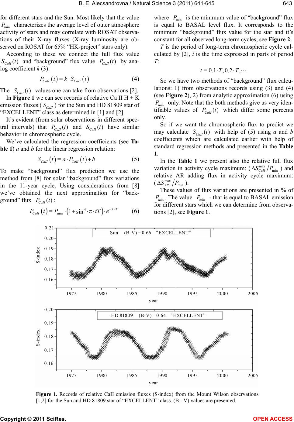

B. E. Alecsandrovna / Natural Science 3 (2011) 641-645

643643

for different stars and the Sun. Most likely that the value

min

P characterizes the average level of outer atmosphere

activity of stars and may correlate with ROSAT observa-

tions of their X-ray fluxes (X-ray luminosity are ob-

served on ROSAT for 65% “HK-project” stars only).

According to these we connect the full flux value

()

CaII

St and “background” flux value ()

CaII

Pt by ana-

log coefficient k (3):

 

CaII CaII

PtkS t (4)

The ()

CaII

St values one can take from observations [2].

In Figure 1 we can see records of relative Ca II H + K

emission fluxes (CaII

S) for the Sun and HD 81809 star of

“EXCELLENT” class as determined in [1] and [2].

It’s evident (from solar observations in different spec-

tral intervals) that ()

CaII

Pt and ()

CaII

St have similar

behavior in chromospheric cycle.

We’ve calculated the regression coefficients (see Ta-

ble 1) a and b for the linear regression relation:

 

CaII CaII

StaPtb (5)

To make “background” flux prediction we use the

method from [8] for solar “background” flux variations

in the 11-year cycle. Using considerations from [8]

we’ve obtained the next approximation for “back-

ground” flux ()

CaII

Pt:



min

=1 π

sin tT

CaII

PtP tTe



  (6)

where min

P is the minimum value of “background” flux

is equal to BASAL level flux. It corresponds to the

minimum “background” flux value for the star and it’s

constant for all observed long-term cycles, see Figure 2.

T is the period of long-term chromospheric cycle cal-

culated by [2], t is the time expressed in parts of period

= 0.1,0.2,tTT





So we have two methods of “background” flux calcu-

lations: 1) from observations records using (3) and (4)

(see Figure 2), 2) from analytic approximation (6) using

min

P only. Note that the both methods give us very iden-

tifiable values of ()

CaII

Pt which differ some percents

only.

So if we want the chromospheric flux to predict we

may calculate ()

CaII

St with help of (5) using a and b

coefficients which are calculated earlier with help of

standard regression methods and presented in the Table

In the Table 1 we present also the relative full flux

variation in activity cycle maximum: (max

min

CaII

SP) and

relative AR adding flux in activity cycle maximum:

(max

min

SP).

These values of flux variations are presented in % of

min

P. The value min

P - that is equal to BASAL emission

for different stars which we can determine from observa-

tions [2], see Figure 1.

Figure 1. Records of relative CaII emission fluxes (S-index) from the Mount Wilson observations

[1,2] for the Sun and HD 81809 star of “EXCELLENT” class. (B - V) values are presented.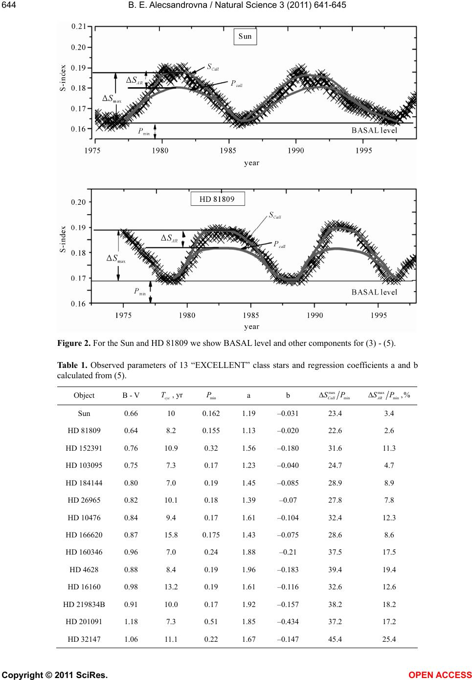

B. E. Alecsandrovna / Natural Science 3 (2011) 641-645

644

Figure 2. For the Sun and HD 81809 we show BASAL level and other components for (3) - (5).

Table 1. Observed parameters of 13 “EXCELLENT” class stars and regression coefficients a and b

calculated from (5).

Object B - V

cyc

T, yr min

P a b max

minCaII

SPmax

min ,%

SP

Sun 0.66 10 0.162 1.19 –0.031 23.4 3.4

HD 81809 0.64 8.2 0.155 1.13 –0.020 22.6 2.6

HD 152391 0.76 10.9 0.32 1.56 –0.180 31.6 11.3

HD 103095 0.75 7.3 0.17 1.23 –0.040 24.7 4.7

HD 184144 0.80 7.0 0.19 1.45 –0.085 28.9 8.9

HD 26965 0.82 10.1 0.18 1.39 –0.07 27.8 7.8

HD 10476 0.84 9.4 0.17 1.61 –0.104 32.4 12.3

HD 166620 0.87 15.8 0.175 1.43 –0.075 28.6 8.6

HD 160346 0.96 7.0 0.24 1.88 –0.21 37.5 17.5

HD 4628 0.88 8.4 0.19 1.96 –0.183 39.4 19.4

HD 16160 0.98 13.2 0.19 1.61 –0.116 32.6 12.6

HD 219834B 0.91 10.0 0.17 1.92 –0.157 38.2 18.2

HD 201091 1.18 7.3 0.51 1.85 –0.434 37.2 17.2

HD 32147 1.06 11.1 0.22 1.67 –0.147 45.4 25.4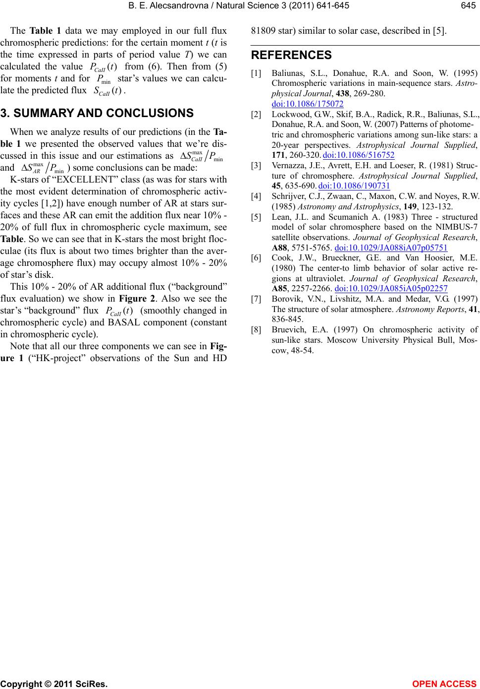

B. E. Alecsandrovna / Natural Science 3 (2011) 641-645

645645

The Table 1 data we may employed in our full flux

chromospheric predictions: for the certain moment t (t is

the time expressed in parts of period value T) we can

calculated the value ()

CaII

Pt from (6). Then from (5)

for moments t and for min

P star’s values we can calcu-

late the predicted flux ()

CaII

St.

3. SUMMARY AND CONCLUSIONS

When we analyze results of our predictions (in the Ta-

ble 1 we presented the observed values that we’re dis-

cussed in this issue and our estimations as max

minCaII

SP

and max

minAR

SP) some conclusions can be made:

K-stars of “EXCELLENT” class (as was for stars with

the most evident determination of chromospheric activ-

ity cycles [1,2]) have enough number of AR at stars sur-

faces and these AR can emit the addition flux near 10% -

20% of full flux in chromospheric cycle maximum, see

Table. So we can see that in K-stars the most bright floc-

culae (its flux is about two times brighter than the aver-

age chromosphere flux) may occupy almost 10% - 20%

of star’s disk.

This 10% - 20% of AR additional flux (“background”

flux evaluation) we show in Figure 2. Also we see the

star’s “background” flux ()

CaII

Pt (smoothly changed in

chromospheric cycle) and BASAL component (constant

in chromospheric cycle).

Note that all our three components we can see in Fig-

ure 1 (“HK-project” observations of the Sun and HD

81809 star) similar to solar case, described in [5].

REFERENCES

[1] Baliunas, S.L., Donahue, R.A. and Soon, W. (1995)

Chromospheric variations in main-sequence stars. Astro-

physical Journal, 438, 269-280.

doi:10.1086/175072

[2] Lockwood, G.W., Skif, B.A., Radick, R.R., Baliunas, S.L.,

Donahue, R.A. and Soon, W. (2007) Patterns of photome-

tric and chromospheric variations among sun-like stars: a

20-year perspectives. Astrophysical Journal Supplied,

171, 260-320. doi:10.1086/516752

[3] Vernazza, J.E., Avrett, E.H. and Loeser, R. (1981) Struc-

ture of chromosphere. Astrophysical Journal Supplied,

45, 635-690. doi:10.1086/190731

[4] Schrijver, C.J., Zwaan, C., Maxon, C.W. and Noyes, R.W.

(1985) Astronomy and Astrophysics, 149, 123-132.

[5] Lean, J.L. and Scumanich A. (1983) Three - structured

model of solar chromosphere based on the NIMBUS-7

satellite observations. Journal of Geophysical Research,

A88, 5751-5765. doi:10.1029/JA088iA07p05751

[6] Cook, J.W., Brueckner, G.E. and Van Hoosier, M.E.

(1980) The center-to limb behavior of solar active re-

gions at ultraviolet. Journal of Geophysical Research,

A85, 2257-2266. doi:10.1029/JA085iA05p02257

[7] Borovik, V.N., Livshitz, M.A. and Medar, V.G. (1997)

The structure of solar atmosphere. Astronomy Reports, 41,

836-845.

[8] Bruevich, E.A. (1997) On chromospheric activity of

sun-like stars. Moscow University Physical Bull, Mos-

cow, 48-54.