

Paper Menu >>
Journal Menu >>
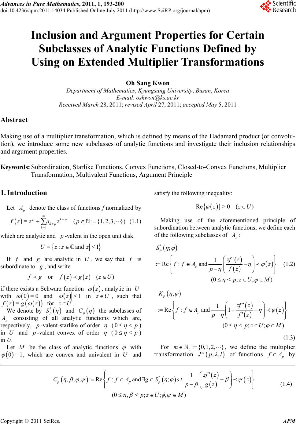 Advances in Pure Mathematics, 2011, 1, 193-200 doi:10.4236/apm.2011.14034 Published Online July 2011 (http://www.SciRP.org/journal/apm) Copyright © 2011 SciRes. APM Inclusion and Argument Properties for Certain Subclasses of Analytic Functions Defined by Using on Extended Multiplier Transformations Oh Sang Kwon Department of Mathematics, Kyungsung University, Busan, Korea E-mail: [email protected] Received March 28, 2011; revised April 27, 2011; accepted May 5, 2011 Abstract Making use of a multiplier transformation, which is defined by means of the Hadamard product (or convolu- tion), we introduce some new subclasses of analytic functions and investigate their inclusion relationships and argument properties. Keywords: Subordination, Starlike Functions, Convex Functions, Closed-to-Convex Functions, Multiplier Transformation, Multivalent Functions, Argument Principle 1. Introduction Let p A denote the class of functions f normalized by =1 =(:{1, 2,3,}) pkp kp k fzza zp (1.1) which are analytic and -valent in the open unit disk p =: and<1Uzz z If f and g are analytic in U, we say that f is subordinate to g , and write or( ) f gfzgzzU if there exists a Schwarz function , analytic in with and z U 0=0 <1z in , such that zU = f zg z for . zU We denote by * p S and p C the subclasses of p A consisting of all analytic functions which are, respectively, -valent starlike of order p (0<p ) in and -valent convex of order U p (0<p ) in U. Let M be the class of analytic functions with , which are convex and univalent in U and 0= 1 satisfy the following inequality: Re> 0()zz U Making use of the aforementioned principle of subordination between analytic functions, we define each of the following subclasses of p A : *; 1 :Re :and (0< ;;) p p S zf z f fA z pfz pz UM (1.2) ; 1 :Re :and1 (0< ;;) p p K zf z f fA z pfz pz UM (1.3) For 0:{0,1, 2,}m , we define the multiplier transformation ,, m J pl of functions p f A by *1 ,;, :Re:and;.. (0,<;; ,) ppp zf z CffAgSst pgz pz UM z (1.4) 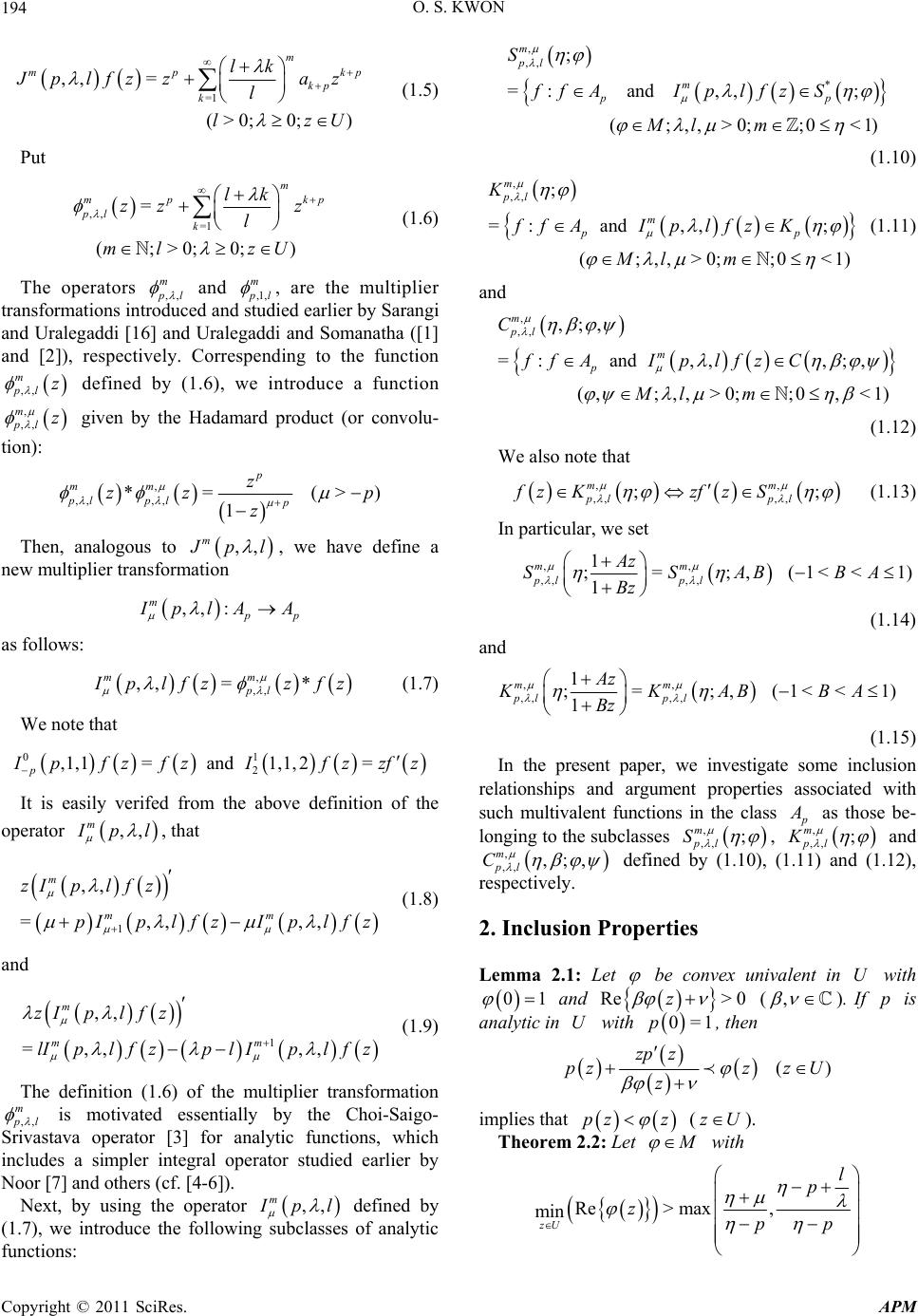 O. S. KWON Copyright © 2011 SciRes. APM 194 =1 ,, = (>0; 0;) m mp kp k lk kp J plfz zaz l lz U (1.5) Put ,, =1 = (;>0;0;) m mp pl k lk zz z l ml zU kp (1.6) The operators ,, m p l and ,1, m p l , are the multiplier transformations introduced and studied earlier by Sarangi and Uralegaddi [16] and Uralegaddi and Somanatha ([1] and [2]), respectively. Correspending to the function ,, m plz defined by (1.6), we introduce a function , ,, m plz given by the Hadamard product (or convolu- tion): , ,, ,, *= (> 1 p mm pl plp z zz z ) p Then, analogous to ,, m J pl , we have define a new multiplier transformation ,, : m p p I plA A as follows: , ,, ,, =* mm pl I plfz zfz (1.7) We note that 01 2 ,1,1=and1,1, 2= p I pfzfz Ifzzf z It is easily verifed from the above definition of the operator ,, m I pl , that 1 ,, =,, ,, m mm zIpl f z pIpl fzIplf z (1.8) and 1 ,, =,, ,, m mm zIplf z lIpl f zplIplf z (1.9) The definition (1.6) of the multiplier transformation ,, m p l is motivated essentially by the Choi-Saigo- Srivastava operator [3] for analytic functions, which includes a simpler integral operator studied earlier by Noor [7] and others (cf. [4-6]). Next, by using the operator ,, m I pl defined by (1.7), we introduce the following subclasses of analytic functions: * =: and ,,; (;,,>0;;0<1 m pp ff AI p lfzS Ml m , ,, ; m pl S ) (1.10) , ,, ; =:and ,,; (;,,>0;;0<1 m pl m pp K ff AI p lfzK Ml m ) (1.11) and ,, ,;, =:and ,,,;, (,;,, >0;;0, <1) pl m p ff AI p lfzC Ml m ,m C (1.12) We also note that ,, ,,pl pl zf zS ,m , ;; m fz K (1.13) In particular, we set ,, ,, ,, 1 mm Az ;=;,(1<<1) 1 pl pl SS ABBA Bz (1.14) and ,, ,, ,, 1 ;= ;,(1<< 1 mm pl pl Az KKABB Bz 1)A (1.15) In the present paper, we investigate some inc re lusion lationships and argument properties associated with such multivalent functions in the class p A as those be- longing to the subclasses , ,, ; m pl S , , ,; , m Kpl and , ,, ,;, m pl C defined(1.12), by (1.10), .11) and (1 respectively. 2. Inclusion Properties emma 2.1: Let L be convex univalent in with U 01 and Re> 0z (, ). Ip is n U f analytic iwith 0=1p, then () zp z pzzz U z implies that pz z 2.2: Let (zU). Theorem M with Re>max, min zU l p zpp 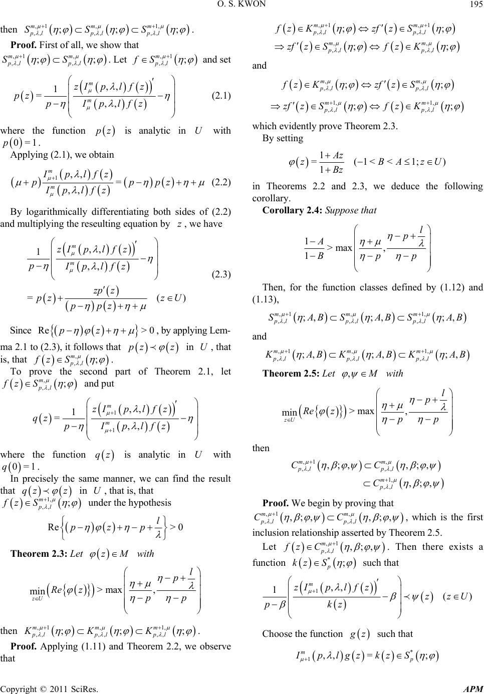 O. S. KWON195 then ; ,1 ,1, ,,,, ,, ;; mmm plpl pl SSS . Proof. First of all, we show that ,1 , ,, ,, ;; mm pl pl SS . Let ,1 ,, ; m pl fS and set ,, 1m zIpl f z =,, m pz pIp fz l (2.1) where the function pz obtain is analytic in with . ng (2.1), we U 0=1p Applyi 1 ,, m pp pz Iplf ,, = m Iplfz z (2.2) tiating both sides of (2.2) and multiplying the reseulting equation by , we have By logarithmically differen z ,, 1 =() m zIplf z zp z pzz U ppz Since , by app ma 2.1 to (2.3), it follows that in , that is, that ,, m pIplfz (2.3) Re> 0pz lying Lem- pz z U , ,, ; m pl fz S . prove the second To parm t of Theore 2.1, let z S , ,, ; m pl f and put 1 1 =,, m qz pIp lfz ,, 1m zIplf z where the function is analytic in with . precisely the sanner, we can ult that in , that is, that qz me ma U find the res 0=1q In qz z U 1, ,, ; m pl fz S unhe hypothesis der t Re> 0pzp t zM with l Theorem 2.3: Le >max , min zU l p Re zpp then ; ,1 ,1, ,,,, ,, ;; mmm plpl pl KKK ,1 ,1 ,, ,, ,, ,, ,, ;; ;; mm pl pl mm pl pl fzKzfzS zfzSf zK and ,, ,,,, ;; mm pl pl fzKzfzS 1, 1, ,, ,, ;; mm pl pl zfzSf zK which evidently prove Theorem 2.3. By setting 1 =(1<<1; 1 Az zBA Bz )zU in Theorems 2.2 and 2.3, we deduce the fo corollary. Corollary 2.4: Suppose that llowing . Proof. Applying (1.11) and Theorem 2.2, we observe that 1>max , 1 l p A Bpp Then, for the function classes defined by (1.12) and (1.13), 1, ,,,,,, ;, m plpl pl SA B and ,1 , ;, ;, mm SABSAB ,1 ,1, ,,,, ,, ;, ;,;, mmm plpl pl K AB KAB KAB Theorem 2.5: Let with , M >max , min zU l p Re zpp then ,1 , ,, ,, ,, ,;, ,;, ;, mm pl pl pl CC C 1, , m Proof. We begin by proving that ,1 , ,, ,, ,;, ,;, mm pl pl CC , which is tfirst inclusion relationship asserted by Theorem 2.5. he Let ,1 ,, ,;, m pl fz C . Then there exists a function ; p kz S * such that 1,, 1() m zIpl f zzzU pkz Choose the function g z such that 1,, = m p Iplgzk *;zS Copyright © 2011 SciRes. APM 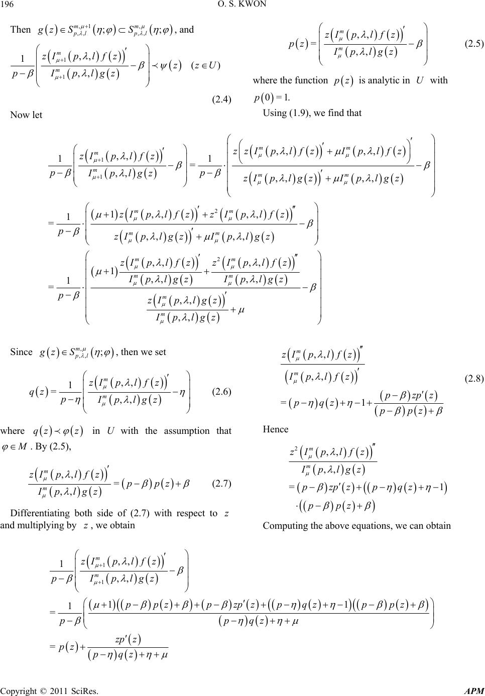 O. S. KWON Copyright © 2011 SciRes. APM 196 Then , ,, ;; pl S ,1 ,, mm pl gz S , and 1 1 ,, 1() ,, m m zIpl f zzzU pIplgz (2.4) Now let ,, =,, m m zIplf z Iplgz pz (2.5) where the function pz is analytic in with U 0=1p. nd th Using (1.9), we fiat 1 1 2 ,, ,, ,, 11 = ,, ,, ,, 1,, ,, 1 = ,, ,, 1 = mm m mmm mm mm zzI p lfzI p lfz zIpl f z pp IplgzzI p lgzI p lgz zIplfzzIplfz pzI p lgzI p lgz p 2 ,, ,, 1,, ,, ,, ,, mm mm m m zIplfz zIplfz Iplgz Iplgz zI p lgz Iplgz Since , ,, ; m pl gz S , then we set ,, 1 =,, m m zIplf z qz pIplgz ,, ,, =1 m m zI p lfz Iplfz pzpz pqz ppz (2.8) Hence (2.6) w in Uumption that here q with the ass z z M . By (2.5), 2,, ,, =1 m m zI plfz Iplgz pzpzpqz ppz ,, = ,, m m zIpl f zppz Iplgz and mu, we obtain (2.7) Differentiating both side of (2.7) with respect to z ltiplying by zComputing the above equations, we can obtain 1 1 ,, 1 ,, = m m zIpl f z pIplgz pz ppqz zp z pz pqz 1 1 =pp z pz 1 pqz ppz 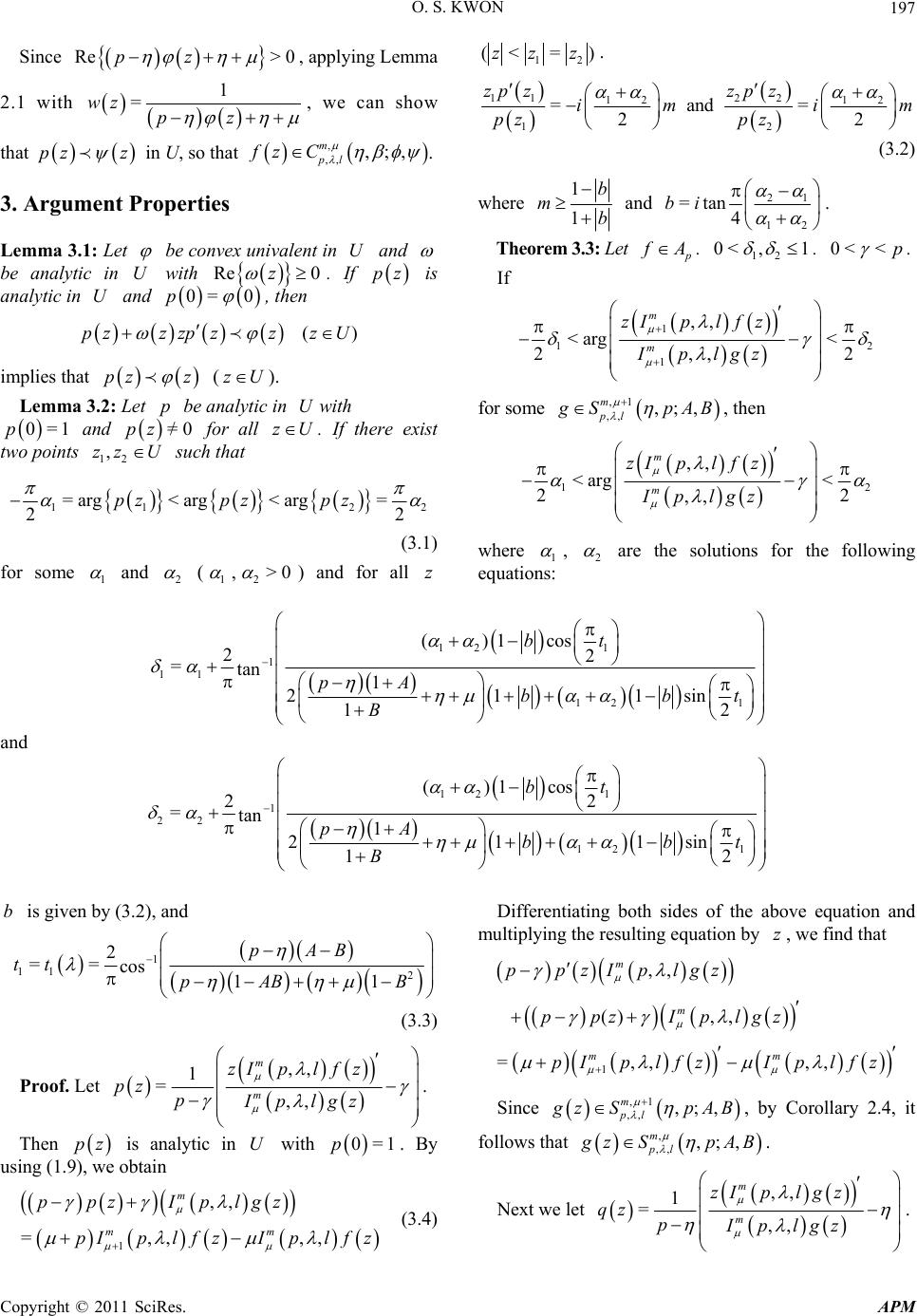 O. S. KWON197 Since , applying Lemma 2.1 wit Re> 0pz h 1 =wz pz , we can show that p zz in U, so that , ,, ,;, m pl fz C . 3. Argument Properties emma 3.1: Let L be convex univalent in and U betic in with analy U Re z 0. If pz is analytic in U and 0= 0 , thepn )pzz U (zzp zz impli z (z es that pz U ). Lemma 3.2: Let be analytic in with p U 0=1p and =0pz for o points ,zz U such that all . If there exist zU tw 12 11 22 =arg <arg 2 p pz <arg=z pz2 (3.1) for some 1 and 2 (1 ,2>0 ) and fr all oz 12 (<= )zz z . 112 2 12 12 12 =and= 22 zp zzpz im i pz pz m (3.2) where 1 1 b mb and 21 12 =tan 4 bi . Theorem 3.3: Let p f A . 12 0< ,1 . 0<< p . If 1 12 1 ,, <arg < 22 ,, m m zIplf z Iplgz ,1 ,, ,;, m pl g SpA B, then for some 1 <a rg < zI 2 ,, 22 ,, m m pl f z Iplgz where , 2 1 are the solutions for the following equatio ns: 1 1 1 ( 2 =tan 2 )1cb 1 1 12 1 os 2 1 211sin 12 t pA bbt B and 1 1 1 22 12 1 22 =tan1 211sin 12 pA bbt B is given by (3.2), and 2 1cosbt () b 1 11 = tt 2 2 = cos 11 pAB pAB B (3.3) Proof. Let ,, 1 =,, m m zIpl f z pz pIplgz . in with . By using (1we obtain (3.4) Differentiating both sides of the above equation and multiplying the resulting equation by , we find that Then pz is analytic U 0=1p .9), 1 ,, =,, ,, m mm ppz Iplgz pIpl f zIpl fz z 1 ,, (),, =,, ,, m m mm ppzIplgz ppz Iplgz pIplfzI plfz Since ,1 ,, ,;, m pl g zS pAB hat , by Corollary 2.4, it follows t , ,, ,;, m pl g zS pA B. Next we let ,, 1 = m m zI p lgz qz gz ,, pIpl . Copyright © 2011 SciRes. APM 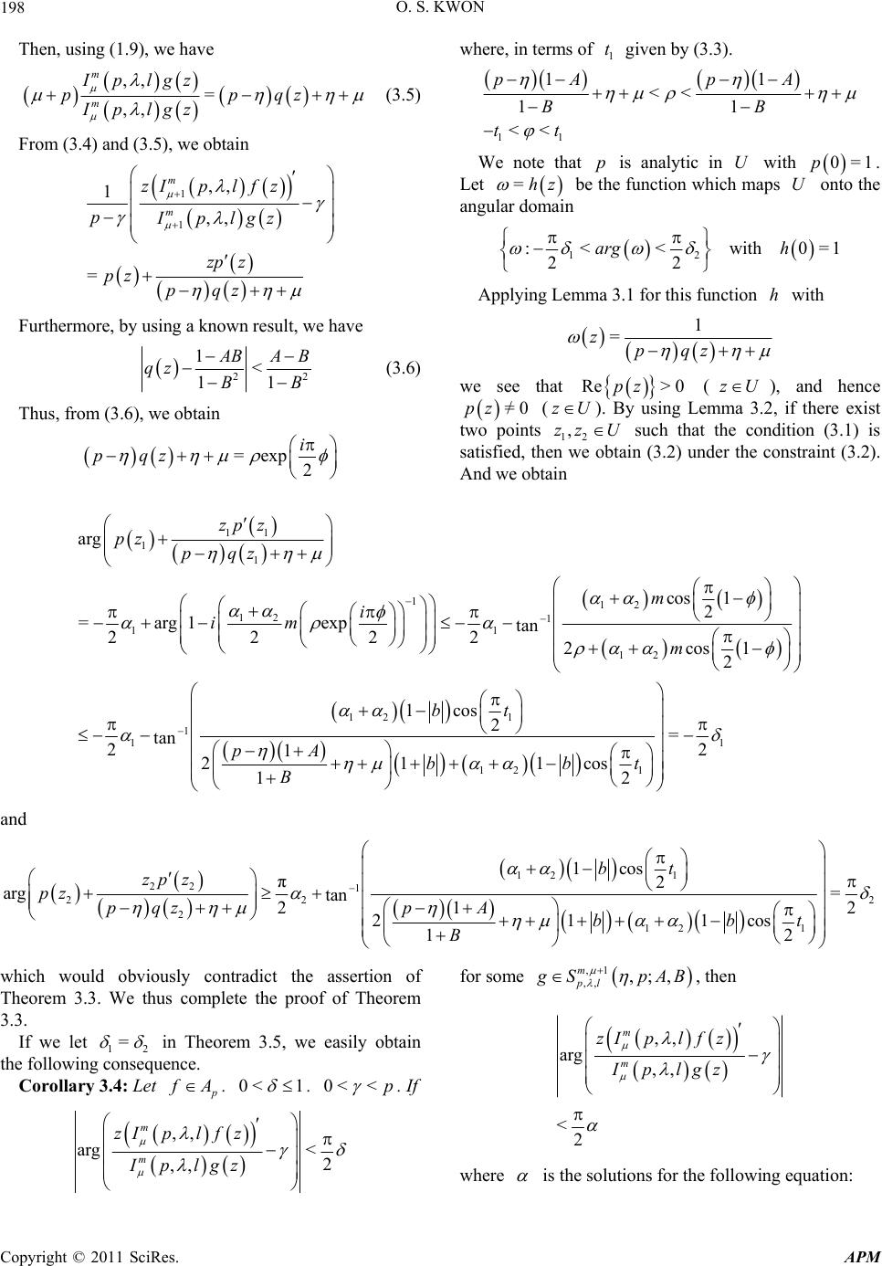 O. S. KWON 198 Then, using (1.9), we have ,, = ,, m m Iplgz ppq Iplgz z (3.5) From (3.4) and (3.5), we obtain 1 1,, = m pIp lgz zp z pz pqz ,, 1m zIplf z Furthermore, by using a known result, we have 22 1< 11 A BAB qz BB (3.6) Thus, from (3.6), we obtain =exp2 i pqz where, in terms of 1 t given by (3.3). 11 <<tt 11 << 11 pA p BB A We note that is analytic in with p U 0=1p. Let =hz lar domain be function whicaps angu theh mU onto the 12 :<< with0 22 arg h =1 Applying Lemma 3.1 for this function with h 1 = zpqz we see that e> 0pz (), and hence RzU =0pz (zU ). By using 12 zz U Lem if there exist ma 3.2, two points , such th we obtain (3.2 at the h condition (3) is ) under te constraint (3.2). A .1 satisfied, then nd we obtain 11 1 1 11 12 1 12 12 1 1 1 arg =arg1 exp 222 2 1 1 cos 1 2 tan 2 2c os1 2 1cos 2 tan 21 21 zp z pz pqz i im m bt pA B m 1 12 1 =2 11cos 2 bbt and 12 1 22 1 22 2 2 12 1 1cos π2 arg = tan 22 1 211cos 12 bt zp z pz pqz pA bbt B which would obviously contradict the assertion of Theorem 3.3. We thus complete the proof of Theorem 3.3. If we let 12 = onseque in Theorem 3.5, we easily obtain the following cnce. rollary 3.4: Let Co p f A. 0< 1 . 0<< p . If ,, arg< 2 ,, m m zIpl f z Iplgz ,1 ,, ,;, m pl g SpA B, then for some ,, arg ,, <2 m m zIpl f z Iplgz where is the solutions for the following equation: Copyright © 2011 SciRes. APM 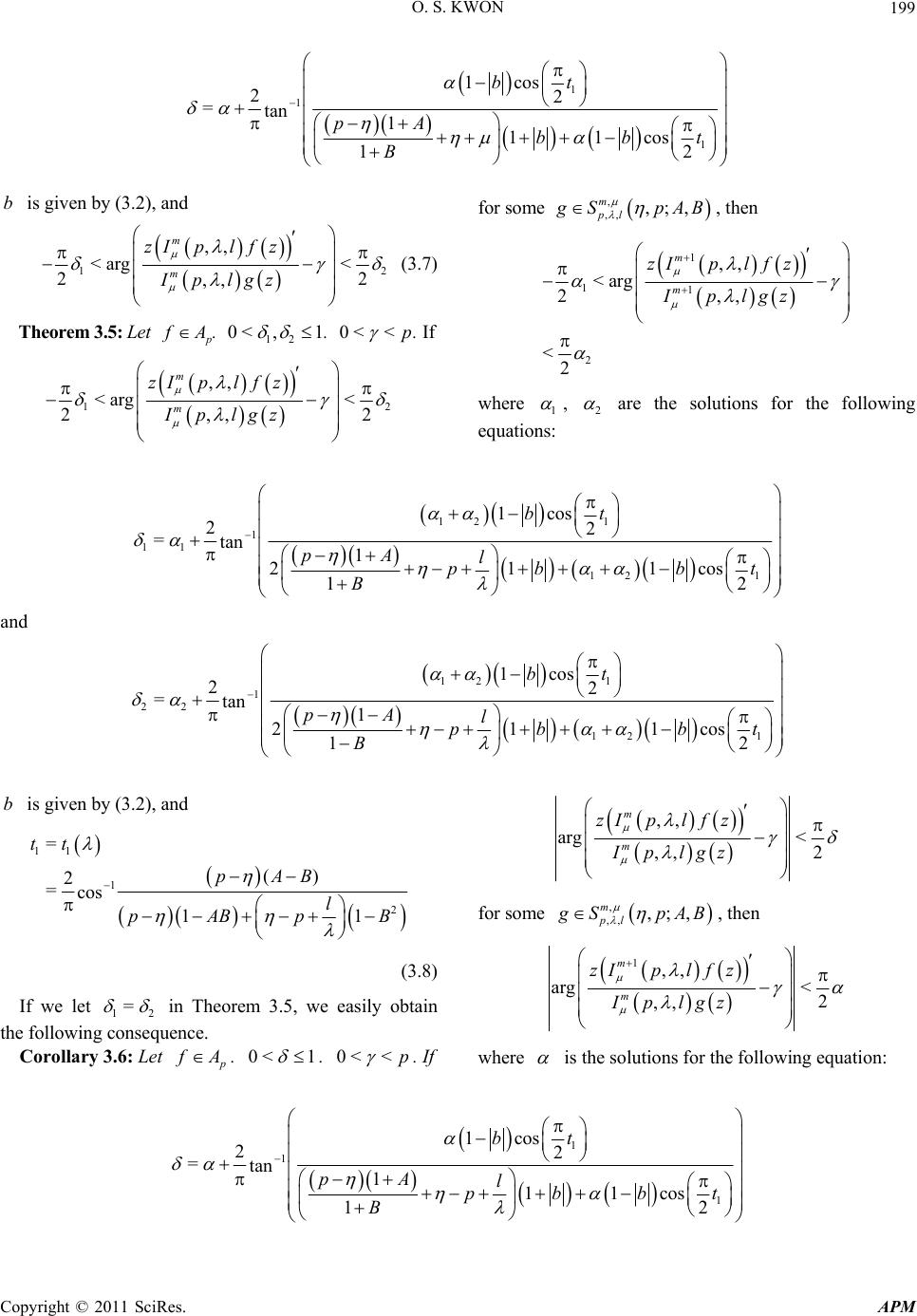 O. S. KWON199 1 1 1 1cos 22 =tan 111cos 12 bt pA bbt B b is given by (3.2), and 1 ,, <arg< 2 m m zIplf z Ip 2 2 ,, lgz (3.7) Theorem 3.5: Let p f A. 12 0< ,1 . 0<<p . If 12 ,, <arg< 22 ,, m m zIplf z Iplgz for some , ,, ,;, m pl g SpA B, then 1 11 2 ,, <arg 2,, <2 m m zIpl f z Iplgz where 1 , 2 are the solutions for the following equations: 12 1 1 11 12 1 1cos 22 =tan 1 211 12 bt pA l pbb B cost and 12 1 1 22 12 1 1cos 22 =tan 1 211cos bt pA lbbt B is given by (3.2), and 12 p b 11 1 2 = () 2 =co s 11 tt pAB l pABp B (3.8) we letIf 12 = in Theorem 3.5, we easily obtain onsequence. Corollary 3.6: Let the following c p f A ,, arg m <2 ,, m zIpl f z Iplgz for some , ,, ,;, m pl g SpA B, then 1,, arg< 2 ,, m m zIplf z Iplgz . 0< 1 . 0<< p . If w here is the solutions for the following equation: 1 1 1 1cos 22 =tan 111cos 12 bt pA l pbb B t Copyright © 2011 SciRes. APM 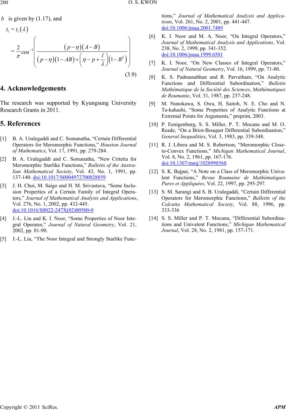 O. S. KWON 200 is given by (1.17), and b 11 1 2 = 2 =cos 1 tt pAB l pABp B 1 (3.9) 4. Acknow The research was supported by Kyungsung University Research Grants in 2011. [1] B. A. Uralegaddi and C. Somanatha, “Certain Differential Operators for Meromorphic Functions,” Houston Journal of Mathematics, Vol. 17, 1991, pp. 279-284. [2] B. A. Uralegaddi and C. Somanatha, “New Critetia for Meromorphic Starlike Functions,” Bulletin of the Austra- lian Mathematical Society, Vol. 43, No. 1, 1991, pp. 137-140. doi:10.1017/S0004972700028859 ledgements 5. References [3 H. M. Srivastava, “Some Inclu- sion Properties of a Certain Family of Integral Ope tors,” Journal of Mathematical Analysis and Applications Vol. 276, No. 1, 2002, pp. 432-445. doi:10.1016/S0022-247X(02)00500-0 ] J. H. Choi, M. Saigo and ra- , [4] J.-L. Liu and K. I. Noor, “Some Properties of Noor Inte- gral Operator,” Journal of Natural Geometry, Vol. 2002, pp. 81-90. [5] J.-L. Liu, “The Noor Integral and Strongly Starlike ” Journal of Mathemalysis and Applica- , Vol. 261, No. 2, 2001, pp. doi:10.1006/jmaa.2001.7489 21, Func- tions, tical Ana tions 441-447. [6] K. I. Noor and M. A. Noor, “On Integral O erators,” Journal of Mathematical Analysis and Applicans, Vol. 238, No. 2, 1999, pp. 341-352. doi:10.1006/jmaa.1999.6501 p tio I” Journal of Natural Geometry, Vol. 16, 1999, pp. 71-80. [8] K. S. Padmanabhan and R. Parvatham, “On Analytic Functions and Differential Subordination,” Bulletin Mathématique de la Société des Sciences, Mathématiques de Roumanie, Vol. 31, 1987, pp. 237-248. [9] M. Nunokawa, S. Owa, H. Saitoh, N. E. Cho and N. Ta-kahashi, “Some Properties of Analytic Functions at Extremal Points for Arguments,” preprint, 2003. [10] P. Eenigenburg, S. S. Miller, P. T. Mocanu and M. O. Reade, “On a Briot-Bouquet Differential Subordination,” General Inequalities, Vol. 3, 1983, pp. 339-348. [11] R. J. Libera and M. S. Robertso “Meromorphic Close- to-Convex Functions,” Michigan , Vol. 8, No. 2, 1961, pp. 167-176. doi:10.1307/mmj/1028998568 [7] K.. Noor, “On New Classes of Integral Operators, n, Mathematical Journal [12] S. K. Bajpai, “A Note on a Class of Meromorphic Univa- lent Functions,” Revue Roumaine de Mathématiques u, “Differential Subordina- Pures et Appliquées, Vol. 22, 1997, pp. 295-297. S. M. Sarangi and[13] S. B. Uralegaddi, “Certain Differential Operators for Meromorphic Functions,” Bulletin of the Calcutta Mathematical Society, Vol. 88, 1996, pp. 333-336 [14] S. S. Miller and P. T. Mocan tions and Univalent Functions,” Michigan Mathematical Journal, Vol. 28, No. 2, 1981, pp. 157-171. Copyright © 2011 SciRes. APM |