The Clouds Microstructure and the Rain Stimulation by Acoustic Waves

doi:10.4236/acs.2011.13009

Paper Menu >>

Journal Menu >>

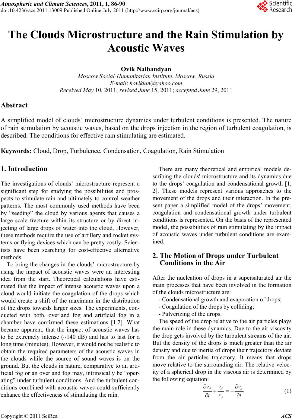Atmospheric and Climate Sciences, 2011, 1, 86-90

doi:10.4236/acs.2011.13009 Published Online July 2011 (http://www.scirp.org/journal/acs)

The Clouds Microstructure and the Rain Stimulation by

Acoustic Waves

Ovik Nalbandyan

Moscow Social-Humanitarian Institute, Moscow, Russia

E-mail: [email protected]

Received May 10, 2011; revised June 15, 2011; accepted J une 29, 2011

Abstract

A simplified model of clouds’ microstructure dynamics under turbulent conditions is presented. The nature

of rain stimulation by acoustic waves, based on the drops injection in the region of turbulent coagulation, is

described. The conditions for effective rain stimulating are estimated.

Keywords: Cloud, Drop, Turbulence, Condensation, Coagulation, Rain Stimulation

1. Introduction

The investigations of clouds’ microstructure represent a

significant step for studying the possibilities and pros-

pects to stimulate rain and ultimately to control weather

patterns. The most commonly used methods have been

by “seeding” the cloud by various agents that causes a

large scale fracture within its structure or by direct in-

jecting of large drops of water into the cloud. However,

these methods require the use of artillery and rocket sys-

tems or flying devices which can be pretty costly. Scien-

tists have been searching for cost-effective alternative

methods.

To bring the changes in the clouds’ microstructure by

using the impact of acoustic waves were an interesting

idea from the start. Theoretical calculations have esti-

mated that the impact of intense acoustic waves upon a

cloud would initiate the coagulation of the drops which

would create a shift of the maximum in the distribution

of the drops towards larger sizes. The experiments, con-

ducted with both, overland fog and artificial fog in a

chamber have confirmed these estimations [1,2]. What

became apparent, that the impact of acoustic waves has

to be extremely intense (~140 dB) and has to last for a

long time (minutes). However, it would not be realistic to

obtain the required parameters of the acoustic waves in

the clouds while the source of sound waves is on the

ground. But the clouds in nature, comparative to an arti-

ficial fog or an overland fog may, intrinsically be “oper-

ating” under turbulent conditions. And the turbulent con-

ditions combined with acoustic waves could sufficiently

enhance the effectiveness of stimulating the rain.

There are many theoretical and empirical models de-

scribing the clouds' microstructure and its dynamics due

to the drops’ coagulation and condensational growth [1,

2]. These models represent various approaches to the

movement of the drops and their interaction. In the pre-

sent paper a simplified model of the drops’ movement,

coagulation and condensational growth under turbulent

conditions is represented. On the basis of the represented

model, the possibilities of rain stimulating by the impact

of acoustic waves under turbulent conditions are exam-

ined.

2. The Motion of Drops under Turbulent

Conditions in the Air

After the nucleation of drops in a supersaturated air the

main processes that have been involved in the formation

of the clouds microstructure are:

- Condensational growth and evaporation of drops;

- Coagulation of the drops by colliding;

- Pulverizing of the drops.

The speed of the drop relative to the air particles plays

the main role in these dynamics. Due to the air viscosity

the drop gets involved by the turbulent streams of the air.

But the density of the drops is much greater than the air

density and due to inertia of drops their trajectory deviate

from the air particles trajectory. It means that drops

move relative to the surrounding air. The relative veloc-

ity of a spherical drop in the viscous air is determined by

the following equation:

dd a

vv v









 (1)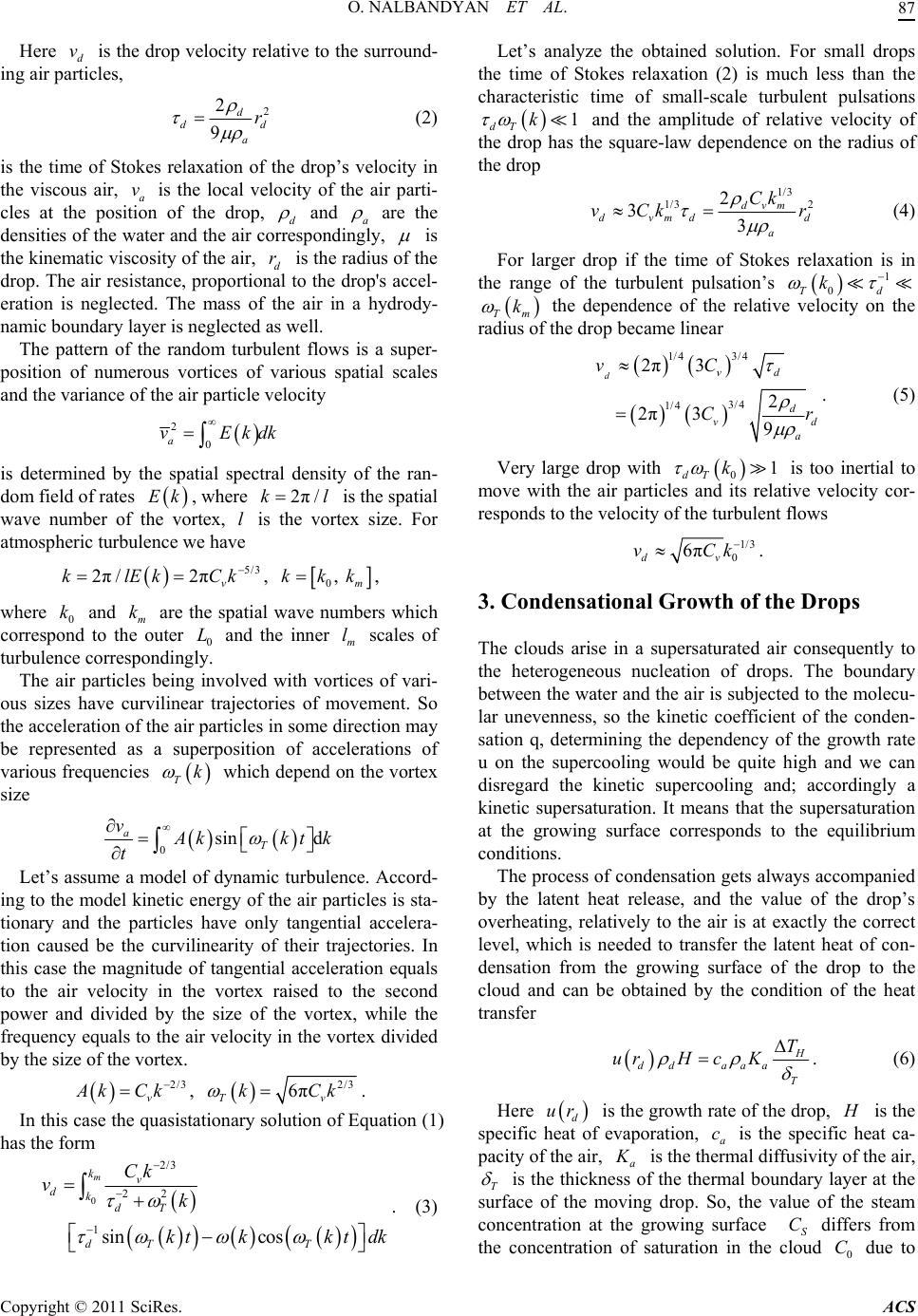

O. NALBANDYAN ET AL.87

Here dis the drop velocity relative to the surround-

ing air particles,





d

(2)

is the time of Stokes relaxation of the drop’s velocity in

the viscous air, a is the local velocity of the air parti-

cles at the position of the drop, d



and a



are the

densities of the water and the air correspondingly,



the kinematic viscosity of the air, d is the radius of the

drop. The air resistance, proportional to the drop's accel-

eration is neglected. The mass of the air in a hydrody-

namic boundary layer is neglected as well.

The pattern of the random turbulent flows is a super-

position of numerous vortices of various spatial scales

and the variance of the air particle velocity



vEk



dk

is determined by the spatial spectral density of the ran-

dom field of rates , where is the spatial

wave number of the vortex, is the vortex size. For

atmospheric turbulence we have



Ek 2π/k



5/3

2π/2πv

klEkCk



,





0, m

kkk,

where 0 and m are the spatial wave numbers which

correspond to the outer 0 and the inner scales of

turbulence correspondingly.

kk Lm

The air particles being involved with vortices of vari-

ous sizes have curvilinear trajectories of movement. So

the acceleration of the air particles in some direction may

be represented as a superposition of accelerations of

various frequencies which depend on the vortex

size





 

0sin d

kkt





k











Let’s assume a model of dynamic turbulence. Accord-

ing to the model kinetic energy of the air particles is sta-

tionary and the particles have only tangential accelera-

tion caused be the curvilinearity of their trajectories. In

this case the magnitude of tangential acceleration equals

to the air velocity in the vortex raised to the second

power and divided by the size of the vortex, while the

frequency equals to the air velocity in the vortex divided

by the size of the vortex.



2/3

kCk



,



2/3

6π

kCk



.

In this case the quasistationary solution of Equation (1)

has the form



 



2/3

1sin cos

dkdT

dT T

ktkkt dk



 











. (3)

Let’s analyze the obtained solution. For small drops

the time of Stokes relaxation (2) is much less than the

characteristic time of small-scale turbulent pulsations





dTk



 and the amplitude of relative velocity of

the drop has the square-law dependence on the radius of

the drop

1/3

1/3 2

dvm

dvmd a

vCk r





 d

(4)

For larger drop if the time of Stokes relaxation is in

the range of the turbulent pulsation’s



0Td













the dependence of the relative velocity on the

radius of the drop became linear



3/4

1/4

3/4

1/4

2π3

2π39

dvd











. (5)

Very large drop with is too inertial to

move with the air particles and its relative velocity cor-

responds to the velocity of the turbulent flows



dTk





1/3

6π

vCk



.

3. Condensational Growth of the Drops

The clouds arise in a supersaturated air consequently to

the heterogeneous nucleation of drops. The boundary

between the water and the air is subjected to the molecu-

lar unevenness, so the kinetic coefficient of the conden-

sation q, determining the dependency of the growth rate

u on the supercooling would be quite high and we can

disregard the kinetic supercooling and; accordingly a

kinetic supersaturation. It means that the supersaturation

at the growing surface corresponds to the equilibrium

conditions.

The process of condensation gets always accompanied

by the latent heat release, and the value of the drop’s

overheating, relatively to the air is at exactly the correct

level, which is needed to transfer the latent heat of con-

densation from the growing surface of the drop to the

cloud and can be obtained by the condition of the heat

transfer



dd aaa

urHcK







. (6)

Here





ur is the growth rate of the drop,

is the

specific heat of evaporation, a is the specific heat ca-

pacity of the air, a

is the thermal diffusivity of the air,



is the thickness of the thermal boundary layer at the

surface of the moving drop. So, the value of the steam

concentration at the growing surface S differs from

the concentration of saturation in the cloud due to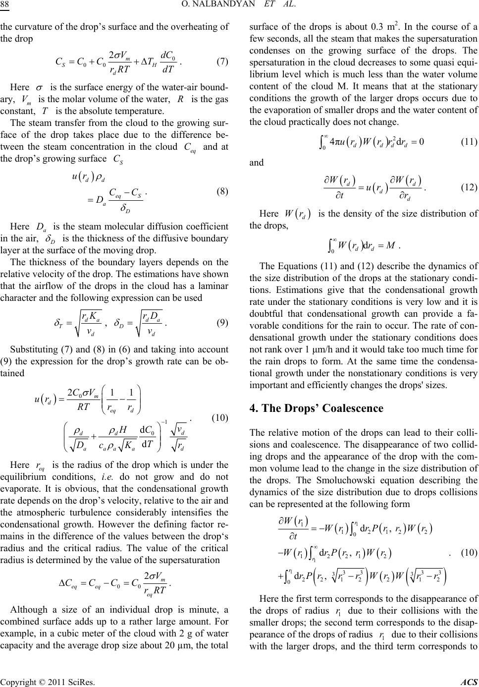

O. NALBANDYAN ET AL.

the curvature of the drop’s surface and the overheating of

the drop

CCC T

rRT dT



 C

. (7)

Here



is the surface energy of the water-air bound-

ary, m is the molar volume of the water, is the gas

constant, is the absolute temperature.

The steam transfer from the cloud to the growing sur-

face of the drop takes place due to the difference be-

tween the steam concentration in the cloud and at

the drop’s growing surface



eq S







. (8)

Here is the steam molecular diffusion coefficient

in the air,



is the thickness of the diffusive boundary

layer at the surface of the moving drop.

The thickness of the boundary layers depends on the

relative velocity of the drop. The estimations have shown

that the airflow of the drops in the cloud has a laminar

character and the following expression can be used



, da



. (9)

Substituting (7) and (8) in (6) and taking into account

(9) the expression for the drop’s growth rate can be ob-

tained



211

deq d

aaaa d

ur RTr r

Dc Kr

























. (10)

Here eq is the radius of the drop which is under the

equilibrium conditions, i.e. do not grow and do not

evaporate. It is obvious, that the condensational growth

rate depends on the drop’s velocity, relative to the air and

the atmospheric turbulence considerably intensifies the

condensational growth. However the defining factor re-

mains in the difference of the values between the drop‘s

radius and the critical radius. The value of the critical

radius is determined by the value of the supersaturation

eq eqeq

CCCC

rRT



.

Although a size of an individual drop is minute, a

combined surface adds up to a rather large amount. For

example, in a cubic meter of the cloud with 2 g of water

capacity and the average drop size about 20 µm, the total

surface of the drops is about 0.3 m2. In the course of a

few seconds, all the steam that makes the supersaturation

condenses on the growing surface of the drops. The

spersaturation in the cloud decreases to some quasi equi-

librium level which is much less than the water volume

content of the cloud M. It means that at the stationary

conditions the growth of the larger drops occurs due to

the evaporation of smaller drops and the water content of

the cloud practically does not change.

 

04πd

dddd

ur Wrrr



0 (11)

and



 

Wr Wr







. (12)

Here





Wr is the density of the size distribution of

the drops,



Wr rM



.

The Equations (11) and (12) describe the dynamics of

the size distribution of the drops at the stationary condi-

tions. Estimations give that the condensational growth

rate under the stationary conditions is very low and it is

doubtful that condensational growth can provide a fa-

vorable conditions for the rain to occur. The rate of con-

densational growth under the stationary conditions does

not rank over 1 μm/h and it would take too much time for

the rain drops to form. At the same time the condensa-

tional growth under the nonstationary conditions is very

important and efficiently changes the drops' sizes.

4. The Drops’ Coalescence

The relative motion of the drops can lead to their colli-

sions and coalescence. The disappearance of two collid-

ing drops and the appearance of the drop with the com-

mon volume lead to the change in the size distribution of

the drops. The Smoluchowski equation describing the

dynamics of the size distribution due to drops collisions

can be represented at the following form



 





12122

12212

33 33

22 12212

Wr WrrPr rWr

WrrPr rWr

rP rrrWrWrr















. (10)

Here the first term corresponds to the disappearance of

the drops of radius 1 due to their collisions with the

smaller drops; the second term corresponds to the disap-

pearance of the drops of radius 1 due to their collisions

with the larger drops, and the third term corresponds to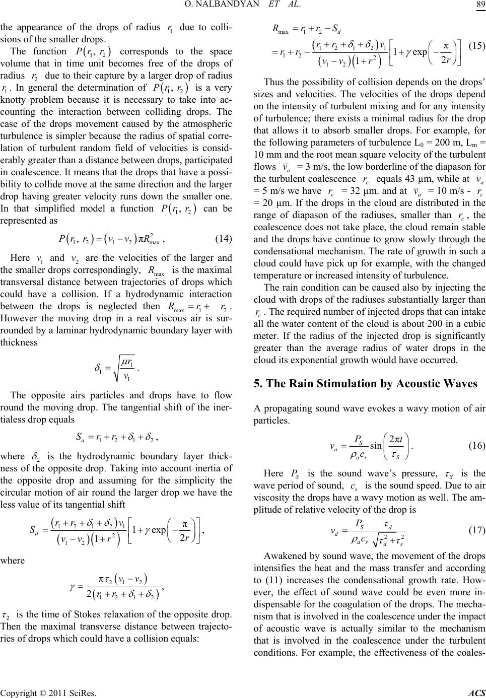

O. NALBANDYAN ET AL.89

the appearance of the drops of radius due to colli-

sions of the smaller drops.



, Pr

The function corresponds to the space

volume that in time unit becomes free of the drops of

radius 2 due to their capture by a larger drop of radius

1. In general the determination of 2

is a very

knotty problem because it is necessary to take into ac-

counting the interaction between colliding drops. The

case of the drops movement caused by the atmospheric

turbulence is simpler because the radius of spatial corre-

lation of turbulent random field of velocities is consid-

erably greater than a distance between drops, participated

in coalescence. It means that the drops that have a possi-

bility to collide move at the same direction and the larger

drop having greater velocity runs down the smaller one.

In that simplified model a function can be

represented as



, Prr





, r





1212ma

, πPr rvvR , (14)

Here 1 and 2 are the velocities of the larger and

the smaller drops correspondingly, max is the maximal

transversal distance between trajectories of drops which

could have a collision. If a hydrodynamic interaction

between the drops is neglected then max1 2.

However the moving drop in a real viscous air is sur-

rounded by a laminar hydrodynamic boundary layer with

thickness

v vR

Rrr





.

The opposite airs particles and drops have to flow

round the moving drop. The tangential shift of the iner-

tialess drop equals

12 1a

Srr2



 ,

where 2



is the hydrodynamic boundary layer thick-

ness of the opposite drop. Taking into account inertia of

the opposite drop and assuming for the simplicity the

circular motion of air round the larger drop we have the

less value of its tangential shift



12 1 21

1exp2

rr v

vv r

 

















 



,

where



21 2

12 1 2









 ,



is the time of Stokes relaxation of the opposite drop.

Then the maximal transverse distance between trajecto-

ries of drops which could have a collision equals:



max1 2

12 1 21

12 2

1exp2

RrrS

rr v

rr r

vvr

 



 



 





 





(15)

Thus the possibility of collision depends on the drops’

sizes and velocities. The velocities of the drops depend

on the intensity of turbulent mixing and for any intensity

of turbulence; there exists a minimal radius for the drop

that allows it to absorb smaller drops. For example, for

the following parameters of turbulence L0 = 200 m, Lm =

10 mm and the root mean square velocity of the turbulent

flows a

v = 3 m/s, the low borderline of the diapason for

the turbulent coalescence c equals 43 µm, while at ra

= 5 m/s we have c = 32 µm. and at ra

v = 10 m/s - c

= 20 µm. If the drops in the cloud are distributed in the

range of diapason of the radiuses, smaller than c, the

coalescence does not take place, the cloud remain stable

and the drops have continue to grow slowly through the

condensational mechanism. The rate of growth in such a

cloud could have pick up for example, with the changed

temperature or increased intensity of turbulence.

The rain condition can be caused also by injecting the

cloud with drops of the radiuses substantially larger than

c. The required number of injected drops that can intake

all the water content of the cloud is about 200 in a cubic

meter. If the radius of the injected drop is significantly

greater than the average radius of water drops in the

cloud its exponential growth would have occurred.

5. The Rain Stimulation by Acoustic Waves

A propagating sound wave evokes a wavy motion of air

particles.

2π

sin

aas S











. (16)

Here S is the sound wave’s pressure, S



is the

wave period of sound,

c is the sound speed. Due to air

viscosity the drops have a wavy motion as well. The am-

plitude of relative velocity of the drop is

das ds







 (17)

Awakened by sound wave, the movement of the drops

intensifies the heat and the mass transfer and according

to (11) increases the condensational growth rate. How-

ever, the effect of sound wave could be even more in-

dispensable for the coagulation of the drops. The mecha-

nism that is involved in the coalescence under the impact

of acoustic wave is actually similar to the mechanism

that is involved in the coalescence under the turbulent

conditions. For example, the effectiveness of the coales-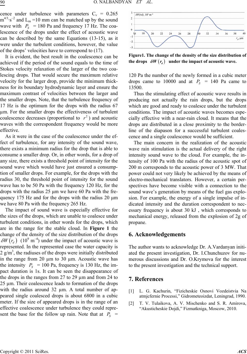

O. NALBANDYAN ET AL.

cence under turbulence with parameters Cv = 0.265

m4/3·s–2 and Lm =10 mm can be matched up by the sound

wave with S = 180 Pa and frequency 17 Hz. The coa-

lescence of the drops under the effect of acoustic wave

can be described by the same Equations (13-15), as it

were under the turbulent conditions, however, the value

of the drops’ velocities have to correspond to (17).

Figure1. The change of the density of the size distribution of

the drops





δWr under the impact of acoustic wave.

It is evident, the best result in the coalescence can be

achieved if the period of the sound equals to the time of

Stokes velocity relaxation of the larger of the two coa-

lescing drops. That would secure the maximum relative

velocity for the larger drop, provide the minimum thick-

ness for its boundary hydrodynamic layer and ensure the

maximum contrast of velocities between the larger and

the smaller drops. Note, that the turbulence frequency of

17 Hz is the optimum for the drops with the radius 67

µm. For the smaller drops the effectiveness of turbulent

coalescence decreases (proportional to ) and acoustic

waves with the correspondent frequency would be more

effective.

120 Pa the number of the newly formed in a cubic meter

drops came to 10000 and at = 140 Pa came to

13500.

Thus the stimulating effect of acoustic wave results in

producing not actually the rain drops, but the drops

which are good and ready to coalesce under the turbulent

conditions. The impact of acoustic waves becomes espe-

cially effective with a near-rain cloud. It means that the

drops are distributed in a close proximity to the border-

line of the diapason for a successful turbulent coales-

cence and a single coalescence would be sufficient.

As it were in the case of the coalescence under the ef-

fect of turbulence, for any intensity of the sound wave,

there exists a minimum radius for the drop that is able to

consume a smaller drop. Or, in other words, for a drop of

any size, there exists a threshold point of intensity for the

sound wave which would have just ensured a consump-

tion of smaller drops. For example, for the drops with the

radius 30, the threshold point of intensity for the sound

wave has to be 50 Pa with the frequency 120 Hz, for the

drops with the radius 25 μm we have 60 Pa with the fre-

quency 175 Hz and for the drops with the radius 20 μm

we have 80 Pa with the frequency 265 Hz.

The main concern in the realization of the acoustic

wave rain stimulation is the actual delivery of the right

intensity sound wave to the cloud. For example, the in-

tensity of 100 Pa with the radius of the acoustic spot of

200 m corresponds to the acoustic power of 3 MW. That

power could not very likely be achieved by the means of

electro-mechanical translators. However, a certain per-

spectives have become visible with a connection to the

sound wave’s generation by means of the fuel gas explo-

sion. For example, the energy of a single impulse of in-

dicated intensity and the duration correspondent to nec-

essary frequency is about 30 kJ , which corresponds to

mechanical energy, released from the explosion of 2g of

propane.

The impact of sound wave is especially effective for

the sizes of the drops, which are unable to coalesce under

turbulent conditions, in other words for the drops, which

are in the range for the stable cloud. In Figure 1 the

change of the density of the size distribution of the drops

(109 m–4) under the impact of acoustic wave is

represented. In the represented case the water capacity is

2 g/m3, the radiuses of the drops were initially distributed

in the range from 20 µm to 30 µm. Acoustic wave has

the intensity S = 100 Pa, frequency is 130 Hz, the im-

pact duration is 1s. It can be seen the disappearance of

the drops in the ranges from 27 to 29 µm and from 24 to

25 µm. Their coalescence leads to formation of the drops

with the radius around 32 µm. A total number of ap-

peared single coalesced drops is about 6800 in a cubic

meter. If the size of appeared drops is in the range of an

effective coalescence under turbulence they could repre-

sent the base for the follow up rain. Note that at =





6. Acknowledgements

The author wants to acknowledge Dr. A.Vardanyan initi-

ated the present investigation, Dr. I.Chunchuzov for nu-

merous discussions and Dr. O.Krymova for the interest

to the present investigation and the technical support.

7. References

[1] L. G. Kachurin, “Fizicheskie Osnovi Vozdeistvia Na

atmjcfernie Processi,” Gidrometeoizdat, Leningrad, 1990.

[2] T. V. Tulaikova, A. V. Mischenko and S. R. Amirova,

“Akusticheskie Dojdi,” Fizmatkniga, Moscow, 2010.