

Journal of Electromagnetic Analysis and Applications
Vol.06 No.10(2014), Article ID:50042,9 pages
10.4236/jemaa.2014.610031
Solution of 1D Poisson Equation with Neumann-Dirichlet and Dirichlet-Neumann Boundary Conditions, Using the Finite Difference Method
Serigne Bira Gueye, Kharouna Talla, Cheikh Mbow
Département de Physique, Faculté des Sciences et Techniques, Université Cheikh Anta Diop, Dakar-Fann, Sénégal
Email: [email protected]
Copyright © 2014 by authors and Scientific Research Publishing Inc.
This work is licensed under the Creative Commons Attribution International License (CC BY).
http://creativecommons.org/licenses/by/4.0/



Received 19 May 2014; revised 16 June 2014; accepted 11 July 2014
ABSTRACT
An innovative, extremely fast and accurate method is presented for Neumann-Dirichlet and Dirichlet-Neumann boundary problems for the Poisson equation, and the diffusion and wave equation in quasi-stationary regime; using the finite difference method, in one dimensional case. Two novels matrices are determined allowing a direct and exact formulation of the solution of the Poisson equation. Verification is also done considering an interesting potential problem and the sensibility is determined. This new method has an algorithm complexity of , its truncation error goes like
 , and it is more precise and faster than the Thomas algorithm.
Keywords:
1D Poisson Equation, Finite Difference Method, Neumann-Dirichlet, Dirichlet-Neumann, Boundary Problem, Tridiagonal Matrix Inversion, Thomas Algorithm

1. Introduction
Poisson equation is used to describe, in quantitative manner, electrostatic and magnetostatic phenomena. It also helps to understand diffusion and propagation related problems, in quasi-stationary regime. Its solution is of great interest for a wide range of fields such as engineering, physics, mathematics, biology, chemistry, etc.
Most of solving methods, of this very important equation, use matrix inversion technics and algorithms, which are dependent on its Right-Hand Side (RHS). A recent study [1] , concerning the case of one dimension, has proposed a direct, exact, and closed formulation of the inverse matrix; independently on the RHS. This inverse matrix has allowed getting a new, extremely fast solution to the Poisson equation. However, this innovative solution, obtained with the finite difference method, discussed only the case of boundary conditions of type: Dirichlet-Dirichlet (DD).
In the present study, we focus on the Poisson equation (1D), particularly in the two boundary problems: Neumann-Dirichlet (ND) and Dirichlet-Neumann (DN), using the Finite Difference Method (FDM). Essentially, attention is given to the matrices extracted from the algebraic equations from this differential method. Furthermore, an exact formulation of their inverses, independently of the RHS, is determined. Therefore, a new and advanced formulation of the solution to the Poisson equation, is found, for Neumann boundary conditions.
The proposed method is more accurate and faster than the Gaussian elimination method and that of Thomas. In addition, it completes the work made by Gueye S. Bira [1] , where the Dirichlet-Dirichlet problem was presented and treated very rigorously and clearly. Here, we determine two matrices that constitute, with the one in ref. [1] , a set of solutions, which will contribute greatly to the advance of research in the field of numerical solving of differential equations. They will also permit an extremely exact and simple formulation of the solution to the Poisson equation.
We will first consider an ND boundary problem and establish the corresponding algebraic equations coming from the application of the finite difference method, using the centered difference approximation (second order derivative). Then, we will, based on these algebraic equations, and considering the boundary conditions; establish the matrix equation. Thereafter, we discuss the properties of the associated matrix and then, determine its inverse, exactly and independently of the RHS. This will allow a direct and exact formulation of the solution to the Poisson equation for a 1D problem with ND boundary conditions. Complexity, accuracy, and stability are discussed and compared with other methods: Gaussian elimination algorithm and Thomas. Moreover, a verification of this new method is done by considering an interesting potential problem with inhomogeneous ND boundary conditions. The results are compared to the exact analytical solution and show great agreement. A similar approach is followed in the case Dirichlet-Neumann problem. The exact formula of the inverse matrix is determined and also the solution of the differential equation.
2. 1D Poisson Equation with Neumann-Dirichlet Boundary Conditions
We consider a scalar potential  which satisfies the Poisson equation
 , in the interval
 , where
  is a specified function.
  fulfills the Neumann-Dirichlet boundary conditions
 and
and . An appropriate discretization is chosen, as shown in Figure 1.
The mesh is composed of  discrete points belonging to the interval
 ; and an extra, imaginary
point,  , which is not within this range [2] [3] . With the following step size:
 , the mesh points
  are defined by the following relation:
 ,
, . We denote by
  the ap-
proximate value of the desired potential at point :
: . For each point
  in the interval
 , the value of the right-hand side function is:
 .
.
 and
and  are the first and second derivative of the potential function
 , respectively, at point
 . With the centered difference approximation
  [2] [4] , one gets the first derivative:
 (1)
(1)
and the second derivative:

Figure 1. Discretization for Neumann-Dirichlet boundary conditions.
 (2)
(2)
Thus, the discretized 1D Poisson equation becomes a set of algebraic equations:
 (3)
(3)
The boundary  must be carefully handled with the extra imaginary point
 . Combining (1) and (3) for
 , the effect of the imaginary point is eliminated:
 (4)
(4)
One sees that this extra point does not affect the result. It is also to remark that the truncation error goes like  [2] . Therefore, this additional point helps to still use the centered difference approximation, even at boundary point
 .
.
We can introduce the vector  which elements
  are defined by:
 (5)
(5)
Thus, one obtains the following matrix equation:
 (6)
(6)
The centered difference approximation leads to an N × N-matrix  that is diagonally dominant, tridiagonal, negative definite, and symmetric.
3. The Inverse of the Matrix 
The inverse of the matrix , denoted
 , is also symmetric. It has the following properties:
 (7)
(7)
where  is the Kronecker’s delta.
It also holds:
 (8)
(8)
The behavior of the determinant and the co-factor of the matrix  in ref. [1] give us also the following relations:
 (9)
(9)
Using the relations in (7)-(9), we can determine exactly the inverse of the matrix  that is associated with our approximation in case of ND boundary conditions. Thus, the coefficients of
  are determined with:
 (10)
(10)
Equation (10) is also equivalent to:
 (11)
(11)
Equations (10) and (11) contain the same information. We prefer the first because it appears to be simpler than the latter and can be preferred for an eventual implementation in a programming language.
Thus, the inverse matrix is entirely determined. We get the simple, beautiful, exact, and very important matrix  that is shown in Figure 2.
We call this impressive matrix , for Neumann-Dirichlet problem: Bira_ND-Matrix. Considering Equation (6), the solution’s vector is obtained with:
 . Thus, solving the 1D Poisson equation is reduced to a simple matrix-vector multiplication. One does not need an inversion method that depend on the right hand side of the differential equation. Further, the interesting properties of this matrix allow us to get the closed formulation of the solution, directly without matrix multiplication.
4. Analysis and Exact Solution of the Poisson Equation
The matrix  is simple and elegant. Only the
  first nonzero integers appear in the matrix
 . Its deeper analysis leads to an exact, closed, and high precise formulation of the solution vector
 , of the Poisson equation.
With Equation (6), one obtains the solution  at point
  with:
with:
 (12)
(12)
The scalar potential  at abscissa
  is given by:
 (13)
(13)
Thus, the solution of the 1D Poisson equation, in the case of Neumann-Dirichlet boundary, is determined exactly with the direct relation:
 (14)
(14)
This is equivalent to:
 (15)
(15)

Figure 2. Inverse matrix for Neumann-Dirichlet problem.
Equation (15) represents a great improvement for solving the Poisson equation, particularly for Neumann- Dirichlet boundary conditions. The solution is determined properly, exactly, and given in a direct formulation. It can be very easily programmed. One loop will be largely sufficient to compute all the solution of one the most important equation in physics and engineering, in the one-dimensional case. It is a novel and exact formulation of the solution with the finite difference method using the centered difference approximation. The very important matrix  allowed us to obtain this innovative solution.
The methods that use inversion technics to obtained the matrix  (Gauss Elimination
 , Thomas Method
  are ameliorated [5] .
The presented new solution is more direct, more exact, more stable; and faster than the Thomas Method for 1D Poisson equation. An important fact is that the determination of  does not depend on the right-hand side of the inhomogeneous Poisson equation. While the other methods use an inversion depending on the RHS of the differential equation. Also, this new solution is very economical with respect to the memory occupation. Then, the solution of the 1D Poisson equation can be got, plotted, and exploited without declaring or using an array in a programming code. That is a great improvement in term of efficient use of memory allocation. Now, we can verify the method, using a potential problem with ND boundary conditions.
5. Verification with a Neumann-Dirichlet Potential Problem
We consider a scalar field , which satisfies
 ,
,
in , where
 ,
,  ,
,  ,
,  , and
, and  are specified real constants.
  fulfills the Neumann-Dirichlet boundary conditions: the values
  and
and  are given. The exact solution is
 (16)
(16)
We can apply the finite difference method, taking: ,
,  ,
,  ,
,  ,
, . We define the mesh according to Figure 1, with
 ,
,  ,
,  ,
,  , and
, and . We consider inhomogeneous Neumann-Dirichlet Boundary conditions:
  and
and .
.
Then, we compute the solution, with new method, given by Equation (15) and compare it with the exact potential (Equation (16)). Naturally, we also take into account the Equation (5).
We denote by  the relative error at point
 , for
, for .
.  is the potential value calculated with the new method i.e.
 , at mesh point
 .
.
For a given , the relative error is obtained according the follow relation:
 (17)
(17)
The denote  the average value of the relative error for a given
 . It is defined by:
 (18)
(18)
It is calculated for the given parameters and its value is: . This is a very good accuracy and corresponds to the results we expected.
Table 1 illustrates the potential , calculated at the position
  by the method of finite differences using
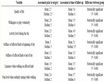
Table 1. Results of the Neumann-Dirichlet problem..
the centered approximation. It also gives the exact value of the potential , obtained by considering the Equation (16) and the relative error at mesh point
 .
.
We see that the solution of the ND boundary problem with the proposed method is also very accurate as shown in the table above.
At this stage, we are interested in the sensitivity of this method. We have shown the average relative error  for different values of
 . Then, we got the curve shown in Figure 3, which is a hyperbola. This func-
tion can be assumed to be proportional to .
.
A curve fitting of the sensibility can be given with:
 (19)
(19)
where . The two curves are shown in Figure 3.
The average relative error  behaves like a truncation error that we express in the following manner
 .
.  is the fourth order derivative of the exact potential function
  in a point (here
 ), which belongs to the interval
 .
.
For the given function  and also the results from the fitting, we have [6] :
 (20)
(20)
6. Solution of Dirichlet-Neumann Problem
6.1. Discretization and Matrix Equation
As we proceeded in the case of boundary conditions of type ND; we will do the same for a DN problem. The first step is to find an adequate and comfortable discretization. We propose that of Figure 4.

Figure 3. Sensibility for the Neumann-Dirichlet problem.

Figure 4. Discretization for Dirichlet-Neumann boundary conditions.
Here, the mesh points  are defined by the following relation:
 ,
, . And,
  and
and  are given. The imaginary point is
 . Its potential
  is eliminated analogically and it holds:
 (21)
(21)
Thus, the vector  can be defined:
 (22)
(22)
Thus, the matrix equation becomes:
 (23)
(23)
In the case of DN boundary conditions, the matrix  is also symmetric, tridiagonal, diagonally dominant, and negative definite. With regard to the anti-diagonal, it is the symmetric of matrix
 , obtained in the case of Neumann-Dirichlet boundary conditions.
6.2. Inverse Matrix and Closed Solution
Thus, the inverse matrix of  can be easily determined from that of the case of ND boundary conditions; using the symmetry in relation to the anti-diagonal. We obtain the beautiful and elegant matrix in Figure 5:
We call this impressive matrix , for Dirichlet-Neumann problem: Bira_DN-Matrix. Thus, the exact expression of the solution of the Poisson equation can be formulated in a very simple manner, as following:
 (24)
(24)
This solution, given by the simple and extremely important Equation (24), can be easily computed, in one programming loop that give all the solutions.
7. Verification with a Dirichlet-Neumann Boundary Problem
We consider the same potential as that of the ND boundary problem, studied above. In this DN problem, the
boundary conditions are:  and
and . The exact solution is obtained by permuting
  and
and  in Equation (16).
We can apply the finite difference method, taking: ,
,  ,
,  ,
,  ,
, . We define the mesh according to Figure 4, with
 ,
,  ,
,  ,
,  , and
, and
 . We consider inhomogeneous DN Boundary conditions:
  and
and .
.
Then, we compute the solution, of our new method, given by Equation (24) and compare it with the exact potential.
Table 2 shows the obtained results:
The solution of the DN problem is also very accurate as shown in Table 2:
 .
.
Table 2. Results of the Dirichlet-Neumann problem.

Figure 5. Inverse matrix for Dirichlet-Neumann problem.

Figure 6. Sensibility for the Dirichlet-Neumann problem.
Now, the sensibility can be determined, for the DN boundary problem: the average relative error  is plotted for different values of
 . Then, we got the hyperbola in Figure 6, which can be assumed to be proportional to
 .
.
A curve fitting of the sensibility can be given using Equation (20) with . The two curves are shown in Figure 6.
The average relative error  goes like
 , which corresponds to the predicted truncation error.
8. Conclusion
This study has determined two novels matrices independently of the RHS providing a new and exact formulation of the solution of the Neumann boundary problem, for the 1D Poisson equation. The presented results and methods constitute a great improvement in the field of solving similar equations: diffusion and wave equations, in the quasi-stationary case, using the FDM. They are direct, highly accurate, extremely fast, and economical in terms of memory occupation.
References
- Gueye, S.B. (2014) The Exact Formulation of the Inverse of the Tridiagonal Matrix for Solving the 1D Poisson Equation with the Finite Difference Method. Accepted Manuscript (JEMAA, April 2014).
- Engeln-Muellges, G. and Reutter, F. (1991) Formelsammlung zur Numerischen Mathematik mit QuickBasic-Program- men, Dritte Auflage, BI-Wissenchaftsverlag, 472-481.
- Kreiss, H.O. (1972) Difference Approximations for Boundary and Eigenvalue Problems for Ordinary Differential Equations. Mathematics of Computation, 26, 605-624. http://dx.doi.org/10.1090/S0025-5718-1972-0373296-3
- LeVeque, R.J. (2007) Finite Difference Method for Ordinary and Partial Differential Equations, Steady State and Time Dependent Problems. SIAM, 15-16. http://dx.doi.org/10.1137/1.9780898717839
- Conte, S.D. and de Boor, C. (1981) Elementary Numerical Analysis: An Algorithmic Approach. 3rd Edition, McGraw- Hill, New York, 153-157.
- Mathews, J.H. and Fink, K.K. (2004) Numerical Methods Using Matlab. 4th Edition, 323-325, 339-342.