Journal of Water Resource and Protection
Vol.4 No.3(2012), Article ID:17949,14 pages DOI:10.4236/jwarp.2012.43018
Optimization Model for Management of Water Quality in a Tidal River Using Upstream Releases
Madras Civil Engineering Department, Environmental and Water Resources Division, 1Professor, Indian Institute of Technology, Chennai, India Madras Civil Engineering Department, Environmental and Water Resources Division
2Indian Institute of Technology Madras Civil Engineering Department, Environmental and Water Resources Division
Email: bsm@iitm.ac.in, tambek72@gmail.com
Received ********* January 3, 2012; revised January 28, 2012; accepted February 29, 2012
Keywords: Water Quality Modeling; Tidal Flow; Simulated Annealing
ABSTRACT
This study deals with the management of water quality in a tidal river through optimal releases of water from an upstream environmental reservoir. A management model is proposed based on the simulation-optimization framework, in which a complete hydrodynamic model for transport of BOD and DO in a tidal river is linked to Simulated Annealing (SA) algorithm for optimization. The proposed management model is used to investigate the effect of tidal variation on the constant minimum in stream discharge that is required to maintain the water quality, for a given pollutant loading. It is demonstrated how the total upstream release volume can be minimized, while still maintaining the desired water quality, by resorting to an optimum temporal variation in releases from the upstream environmental reservoir. The performance of the methodology is evaluated for an illustrative river. The proposed model will be helpful in arriving at best water release policy for maintaining water quality in tidal rivers for given tidal variation and pollutant loading.
1. Introduction
Although the global water crisis tends to be viewed as a water quantity problem, water quality is increasingly being acknowledged as a central factor in the water crisis. Even though not all countries are facing a crisis of water shortage, all have, to a greater or lesser extent, serious problems associated with degraded water quality [1]. In this context, management of water quality along a river system becomes very important. This involves maintenance of acceptable level of water quality for an intended purpose by means of monitoring, assessing, identifying the possible sources of pollution and controlling them accordingly, and diluting by means of upstream releases. In the process of determining the level of problem and devising optimal management strategies, a river water quality model is often employed as a supporting tool in the assessment of aquatic environment. Many efforts have been devoted in the past to the development of water quality management strategies to ensure supply of water with targeted quality [2]. The water quality responses in these management strategies are quantified in terms of the Dissolved Oxygen (DO). Many water quality management models use Streeter-Phelps (S-P) equation for determining the DO in a stream. The Enhanced Stream Water Quality Model (QUAL2E) [3] has been the widely used one for the water quality simulation model.
However these models are limited to a non transient flow conditions that is, it assumes the river flows are steady and quasi-uniform. Management models based on either the S-P equation or the QUAL2E model for simulation of river water quality response have a major limitation in not being applicable to situations where either non-uniform or unsteady flow conditions are significant. Recently, Yandamuri et al. [4] demonstrated the effect of non-uniform flow on optimal waste load allocation decisions in rivers within the framework of a cost-equity based management model. In their study, the flow conditions were non-uniform, but steady.
Although many mathematical models are available for simulation of water quality in river under dynamic conditions, only a few water quality management models have included hydrodynamics within their algorithm structure and can handle transient conditions. Such models are required for managing water quality in a river by dilution using up stream releases from an environmental reservoir or in tidal rivers. Recently, Dhar and Datta [5] developed a management model, where optimal releases from a reservoir were used for controlling the water quality in the downstream river segment. They linked the complete hydrodynamic simulation model, CE-QUAL-W2 to the Genetic Algorithm (GA) based optimization model. The single objective management model developed by them considers the objective of minimizing the summation of normalized squared deviation of actual storage from specified target storage at the end of each management period, subject to the constraint of maintaining water quality standards at downstream control points. The river in their example problem was a non-tidal river, and the target pollutant was nitrate plus nitrite (as N).
In many island countries, countries with limited territory, and in coastal areas, rivers are generally not long, and tidal variations may significantly affect the river water quality. Although several optimization models have been developed and applied for water quality management in the non-tidal rivers, only a few studies have focused on optimal management of water quality in tidal rivers [6]. The use of cyclic discharge of BOD in to a tidal segment and several discharge policies under various tidal cycles that takes advantage of the short time periodic tidal nature of the river in utilizing the capacity of the river to assimilate BOD loading. It was demonstrated that the augmentation of river flow has as much effect on raising DO level as the reduction of point source loadings. Fan et al. [7] assessed the impact of tidal effects on the water quality simulation, and found that usage of the common water quality simulation models without appropriate consideration of the tidal boundary condition may result in a significant discrepancy between the observed and simulated values. All the earlier studies on tidal rivers have highlighted the importance of discharge policy and upstream releases on the water quality, and suggested methods for maintaining the water quality. However, they did not employ any formal optimization technique to arrive at cost effective and efficient management strategies for maintaining water quality.
In this study, maintenance of water quality in a tidal river by optimal releases of water from an upstream environmental reservoir is investigated. A management model, which utilizes a formal optimization technique, is proposed to investigate the effect of tidal variation on the constant minimum in stream discharge that is required to maintain the water quality, for a given pollutant loading. It is also demonstrated how the proposed model can be used to arrive at an optimum temporal variation in releases from an upstream environmental reservoir to maintain the desired water quality. The proposed management model is based on a simulation-optimization framework, where in a complete hydrodynamic model for transport of BOD and DO in a tidal river is linked to Simulated Annealing (SA) algorithm for optimization. It may be noted that although SA has been successfully employed as an optimization tool in several other areas of hydraulic engineering from the earliest [8] to recent work of [9] so far it has had limited application in river water quality management. The performance of the methodology is evaluated for Adyar River in Chennai. The proposed model will be helpful in arriving at best management option for maintaining water quality in tidal rivers for given tidal variation, pollutant loading and water availability in an upstream reservoir.
2. Water Quality Management Model
In this study, a simulation-optimization framework is used to develop the water quality management model. The water quality simulation model is used to determine the spatial and temporal variation in biochemical oxygen demand (BOD) and DO concentrations, for specified inflow (either constant or time varying) at the upstream end, temporal variation of tidal levels at downstream end, waste loading, and channel characteristics. The Simulated Annealing (SA) algorithm is used for obtaining the optimal solutions for reservoir releases.
2.1. Water Quality Simulation Model
The water quality responses to different external interactions and processes in the water environment (i.e. pollutant loading and decay and transport in the river) are simulated using the water quality model. This model consists of two sub-modules: (1) flow module and (2) transport module.
2.1.1. Flow Module
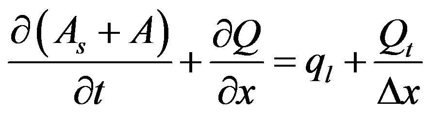
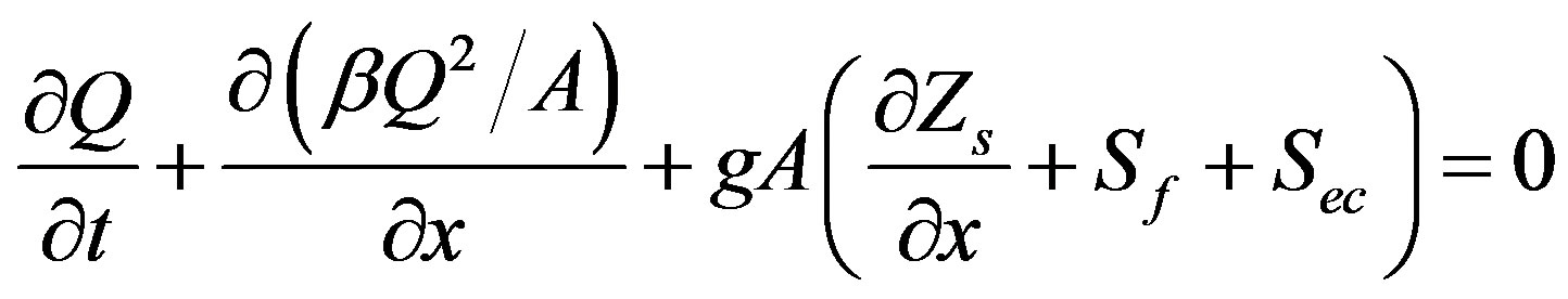
The basic governing equations for river flow considered in the flow module are the St. Venant equations, which represent the conservation of mass and momentum [10]. In this work, long and narrow channels, with possibility of off-channel storage, are considered. These equations, for a one-dimensional flow [11] modified for the effect of the dead storage area are given as:
 (1)
(1)
 (2)
(2)
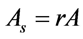
where, Q = main stream flow rate (m3/s), A = main stream cross sectional area (m2), Qt = tributary flow in to the main river (m3/s), ql = lateral flow in to the river along the river stretch (m3/s/m), β = momentum correction factor, Sec = the energy loss due to channel cross sectional shape change (either expansion/constriction), g = gravitational acceleration (m/s2), Sf = friction slope, Zs = the water surface elevation above a given datum (m), and As = the transient storage area in the river banks or dead ends (m2) which contributes only to storage and not to movement of water. As is given as a function of the main channel cross sectional area:
 (3)
(3)
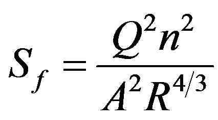
where, r = the ratio of dead storage area to main channel cross sectional area. The friction slope is determined using the Manning equation.
 (4)
(4)
where, R = hydraulic radius, and n = Manning roughness coefficient. It may be noted here that the effect of salinity gradient on the flow is considered to be insignificant in the present work. However, inclusion of the term for salinity effect in momentum equation is not difficult [11]. Equations (1) and (2) are solved numerically for specified initial and boundary conditions. The upstream boundary is the specified inflow hydrograph, while the downstream boundary condition is the specified temporal variation in the water level due to tide. Temporal variation of lateral inflow and tributary inflow is also specified. Arbitrary initial conditions are specified first, and the governing equations are solved for a constant inflow rate at upstream end and corrected for tidal boundary at the downstream end, for a minimum number of tidal cycles (three cycles in the present study). The flow conditions would become steady oscillatory by the end of this time period, and these flow conditions are taken as the initial conditions for further simulations.
In this work, flow equations are solved by the classical Preissmann implicit scheme [10]. Inputs to the flow simulation model are: (1) the geometric characteristics of the river cross sections,; (2) the bed profile of the river, ; (3) the Manning roughness coefficient, ; (4) inflow hydrographs for the main river and the tributaries and (5) tidal levels at the downstream end. For the above input, the flow module simulates temporal and spatial variation in flow area and mean velocity.
2.1.2. Transport Module
This module uses the temporally and spatially varying flow area and flow rate obtained from the flow module for solving the transport equations for BOD and DO. The transport model adapted in the present work considers the exchange of solute (i.e. BOD and DO) between the dead storage zone and the main stream flow zone using decoupled main channel and dead zone transport equations [12]. It is assumed in this study that there is complete mixing in both vertical and transverse directions. This assumption is valid when the flow depth is shallow and the variation of velocity in the vertical direction is not very significant [13]. One-dimensional transport equations for BOD in the main stream and dead storage zone are given by:
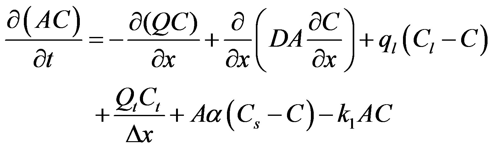 (5)
(5)
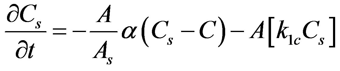 (6)
(6)
The transport equations for DO in the main stream and dead storage zone are given by:
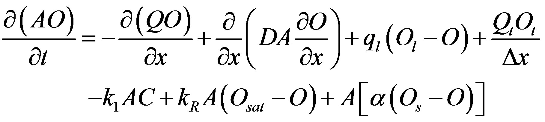 (7)
(7)
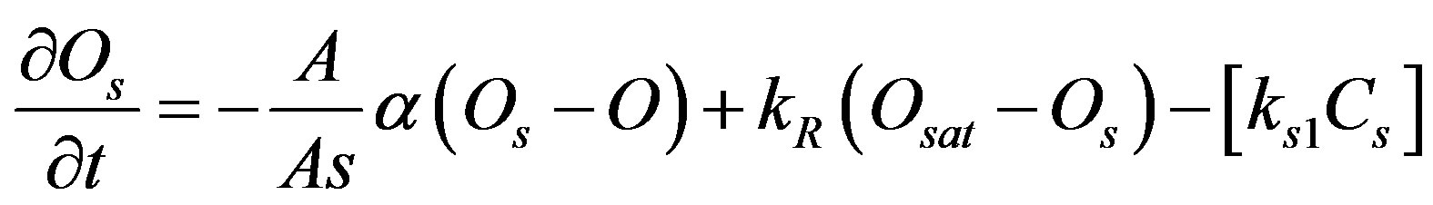 (8)
(8)
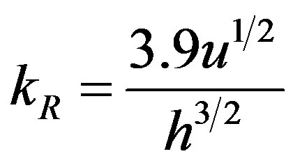
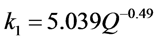
where, C = BOD concentration in the stream (mg/L)Cl = BOD concentration in the lateral inflow (mg/L), D = longitudinal dispersion coefficient (m2/s), Ct = BOD concentration in the tributary in flow (mg/L), Cs = BOD concentration in the storage zone (mg/L), α = stream storage zone solute exchange coefficient, k1 = BOD decay rate coefficient in the stream (1/day), ks1 = BOD decay rate coefficient in the storage zone (1/day), O = concentration of dissolved oxygen in the mainstream, Os = concentration of dissolved oxygen in the storage zone (mg/L), OL = Concentration of dissolved oxygen in the lateral flow (mg/L), Ot = concentration of dissolved oxygen in the tributary flow (mg/L), kR = re-aeration coefficient (1/day), B = bottom width of the channel cross section (m). Fischer’s equation [14] is used for estimating the re-aeration coefficient in Equations (7) and (8), while the decay coefficient in Equations (4) - -(8) are determined using the following equation.
 (9)
(9)
 (10)
(10)
where, u = cross sectional averaged longitudinal flow velocity (m/s) and h = the depth of flow (m). A number of factors affect dispersion in a river system and usually shear-flow dispersion is the dominant. In this study, it is assumed that flow is one dimensional where the longitudinal dispersion dominates. The dispersion coefficient in Equations (5) and (7) are estimated using the following equation proposed by Seo and Cheong [15,16].
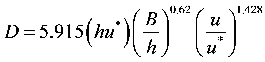 (11)
(11)
where, B = width of the channel, and u* is the friction velocity (m/s), which is given by
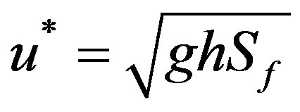 (12)
(12)
The inputs for the transport simulation module consist of 1) initial conditions i.e. spatial variation of BOD and DO at time t = 0, ; 2) boundary conditions i.e. temporal variation of BOD and DO at the upstream and downstream ends, ; 3) pollutant loadings from point and nonpoint sources i.e., temporal variation of Cl, Ct, Ol, and Ot, ; 4) values of system parameters such as ks1, and α,, ; 5) channel characteristics and (v) spatial and temporal variation in flow velocity and flow area, obtained from the solution of Equations (1) and (2). For the above mentioned inputs, Equations (4) - -(7) are solved numerically to obtain spatial and temporal variations of BOD and DO.
The partial implicit-explicit method [1617] is used for the discritization of the partial differential equations. In the discritization process, the transport equations for the dead zone and main stream system are decoupled. First the concentrations of BOD and DO at new time levels in the main stream system are determined, by using concentrations in the dead zone at the known time levels. Concentrations of BOD and DO at new time levels in the main stream system are then substituted in the storage zone transport equation to calculate the concentrations in the dead zone at new time level. At the upstream end, BOD and DO are specified whenever the flow is positive while they are interpolated from interior points when the flow is negative. Similarly, BOD and DO at the downstream end are interpolated from the interior points while they are equal to specified values when the flow is negative. In the present study, they are zero and Osat, respectively, assuming that the BOD in sea is zero owing to dilution. Although a simple boundary condition as described above is implemented at the ocean boundary in this work, it is not difficult to implement a more elaborate boundary condition as described by [1718]. Period of adjustment is allowed by after the flow from ocean starts to flood the river and before the concentration at the mouth reaches the oceanic values.
Water quality simulation models are typically used for simulating the physical and biochemical processes governing water quality in the water bodies. However, simulation models only provide a detailed description of how systems respond to, or are affected by, planning and design solutions, or sets of solutions. Prescription of optimal strategies requires formulation and solution of optimization models [5]. The optimization model used in the present study is described in the following section.
2.2. Optimization Model
The main objective of the present study is to develop a management model for maintaining water quality in a tidal river, by utilizing the releases from an upstream environmental reservoir, for given pollution loading and tidal variation. The optimal operation policy for releases is obtained as a solution of an optimization model. Since water quality is more important in dry periods than in wet periods, the explicit objective of operation is to minimize the total release volume so that water that saved in the environmental reservoir can be used for some other beneficial purpose. The single objective management model formulated in this study considers the objective of minimizing the summation of releases during the operation period, subject to the constraint of maintaining the water quality i.e. the DO concentration above a minimum specified value at all the checking locations in the river. In this study, a simulation-optimization framework is adopted, wherein the simulation model is externally linked to the optimization model and therefore, the number of decision variables is not large. Thus the constraint on DO is incorporated through the externally linked water quality simulation model. The decision variables are the rates of releases and the time durations for which the corresponding releases are maintained. Each day is divided into “M” number of segments of duration. The duration of any segment k (Tk) and the release during that duration (QRel,k) are the decision variables. The transient water quality management model can be mathematically represented as:
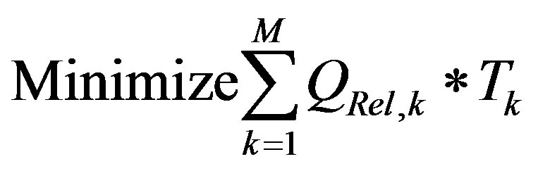 (13)
(13)
It may be noted here that the time horizon for management is taken as three days in all the illustrations in the present study. Each day is divided into M time periods, and the pattern of Tk and corresponding QRel,k on the first day are repeated on the following two days. A time horizon of three days is considered so that the effect of cyclic nature of tidal boundary is incorporated.
Ÿ Simulation constraint. The temporal and spatial variations in the concentrations of BOD and DO in the river depend upon the releases from the upstream environment reservoir. The functional relationship between these variables is specified as a binding equality constraint through the externally linked numerical water quality simulation model:
 (14)
(14)
Wherewhere, 
 is the concentration vector, which includes both BOD and DO,
 is the release vector, and
 is the time duration vector corresponding to releases.
Ÿ Water quality constraint. The concentration of DO at any location j at any time t is more than the minimum required as per standards, DOstd:
 (15)
(15)
Ÿ Reservoir release constraint: The release from the reservoir at any time should not be more than a maximum value, Qmax and less than a minimum value, Qmin which are determined by the channel characteristics.
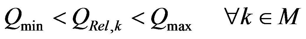 (16)
(16)
The above optimization model for water quality management in the river is solved using a suitable non-linear optimization technique. Simulated Annealing (SA) technique is used for solving the single-objective non-linear optimization model.
2.3. Solution Methodology
A simulation-optimization framework is used in this study for solving the management problem. The simulation model used in this study is the transport and fate numerical hydrodynamic water quality simulation model, described by Equations (1) - -(12). This simulation model is linked to the SA based optimization model. In the linked simulation–-optimization approach, the water quality simulation constraint (Equation (14)) is actually satisfied by numerically solving the water quality simulation model comprising Equations (1) - -(12), linked to the optimization model. The adopted solution methodology is presented schematically in Figure 1.
SA is a generic probabilistic metaheuristic algorithm, developed by [1819] to solve global optimization problems, namely to locate a good approximation to the global minimum of a given function in a large search space. In this method, a configuration consists of a combination of
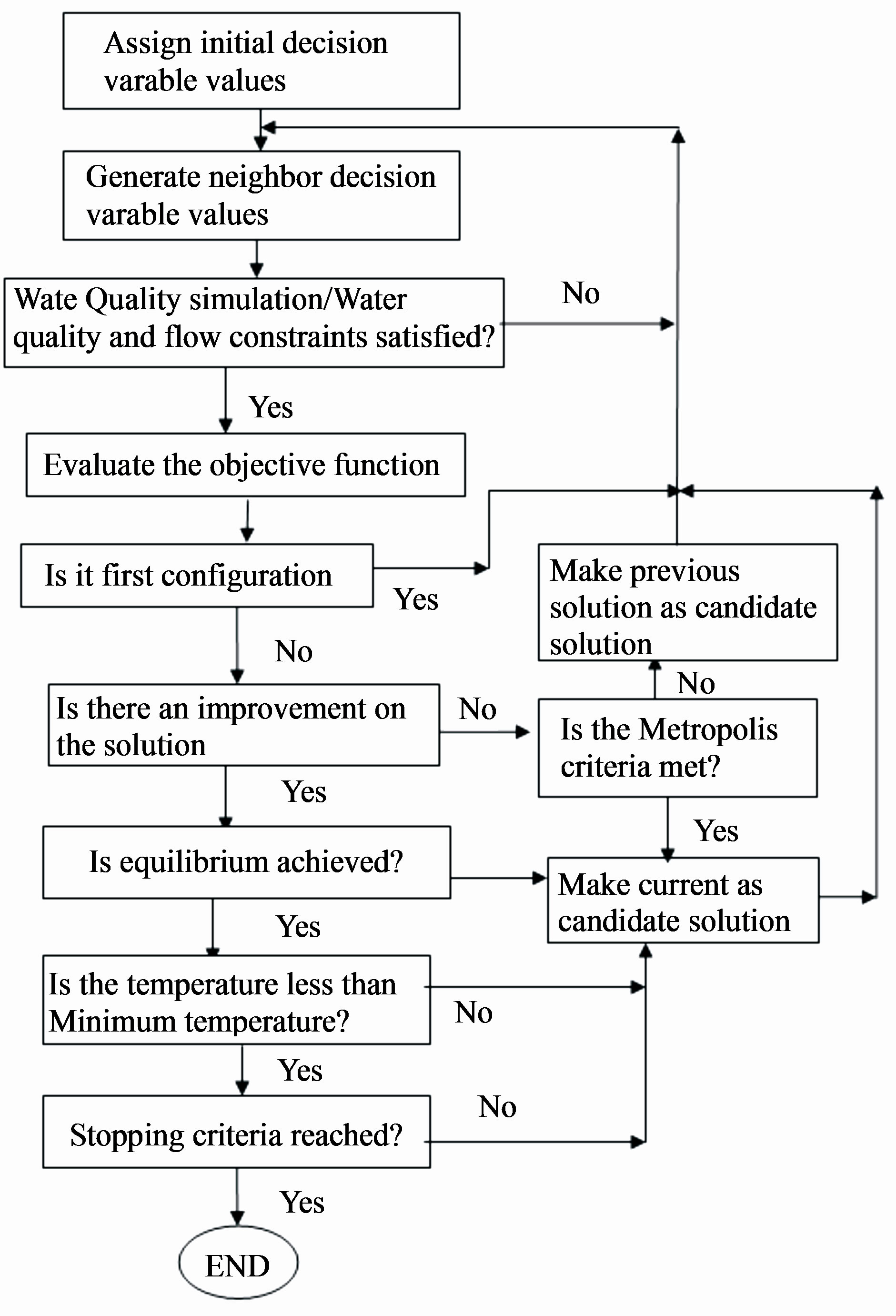
Figure 1. Scheme of solution procedure using simulated annealing.
decision variables, and each decision variable in a combination can only take a discrete value from a set of possible values, specified by the user. Each iteration in the algorithm consists of (1) generation of a random configuration (trial point) within the specified space through perturbation, (; 2) using the water quality simulator to determine the state variables, ; and (3) evaluation of the objective function and constraints. To begin with, the decision variables are initialized by the user, and an initial objective function value is computed. The same values of decision variables are used by the simulation model to evaluate the constraints. The decision variables are then perturbed in the neighborhood and a new configuration is generated. The objective function value and the constraints corresponding to this new configuration are evaluated, once again using the simulator. The current configuration is rejected if it results in constraint violation, a new configuration is generated, and the process is repeated. If the current configuration does not result in constraint violation, and the corresponding objective function value is better than the previous best record, then the current configuration is accepted and the record for best value is updated. A new configuration is then generated, and the process is repeated. If the current configuration does not result in constraint violation, but the corresponding objective function value is worse than the best value available so far, then the acceptance or rejection of the current configuration is decided based on Metropolis criterion and a parameter known as “temperature”, T. Once the decision regarding acceptance or rejection is taken, a new configuration is again generated, and the process is repeated. Metropolis criterion for the acceptance or rejection of uphill moves is implemented by first generating a random deviate, which is uniformly distributed on the interval (0, 1). The worse or “uphill” move is accepted if this random deviate is smaller than the acceptance probability. The probability of acceptance is given by , where ∆E = difference in objective function values corresponding to the current and previous best configurations. The initial value of temperature T is taken large so that a large percentage of uphill moves are also accepted in the initial stages. In the course of iterations, the value of T is progressively lowered so that the acceptance probability of uphill moves in the final stages of iterations is almost equal to zero. The entire iteration process is terminated after a fairly large number of iterations. The allowance for “uphill” moves in the initial stages saves the method from getting stuck at local minima.
3. Validation of the Simulation Model
The water quality simulation model is internally used as a sub-module in the optimization model to determine the stream water quality response for given pollution loading and in stream flow conditions. In this work, different components of adapted water quality simulation model are validated using bench mark solutions available in literature. Although the focus of this study is on optimal management of water quality, a few validation results for flow simulation module are presented here for the sake of completeness. The flow simulation module is validated for a transient flow condition, while the transport and transformation module is validated for a non conservative pollutant i.e., BOD and DO in a single reach of the channel.
3.1. Flow Model
The adapted flow simulation module is validated for transient flow conditions using the data provided by [1920] for an example problem.
Validation Example-1
In this example, the flow at the upstream boundary increases linearly from 224 m3/s - 710 m3/s over a period of 20 minutes. Then it decreases linearly back to its original value over the next 40 minutes, and then remain constant. A uniform flow condition is imposed at the downstream boundary. The time step used in the simulation is 15 seconds. The hydrodynamic data for this example are presented in Table 1.
The flow hydrographs at a distance of 11,000 m from the upstream end obtained analytically [1920] and numerically, are compared in Figure 2. It can be observed from this figure that the performance of the flow model used in the simulation process is satisfactory. There is only a slight attenuation of the peak flow due to numerical diffusion errors.
3.2. Contaminant Transport Model
Transport module is validated for two different pollutant loading cases adopted from literature [2021-2223] and [4]. These loading cases correspond to: time varying loading of BOD and DO at the upstream boundary (Validation Example-2).
Validation Example-2
The ability of the adapted model to simulate the effect of the temporal variation of DO and BOD at the upstream end on the spatial and temporal variation of DO and BOD in the river is tested. In this example problem, a sinusoidal variation in the concentrations of DO is specified as the upstream boundary condition, while zero gradient condition in concentrations is specified at the
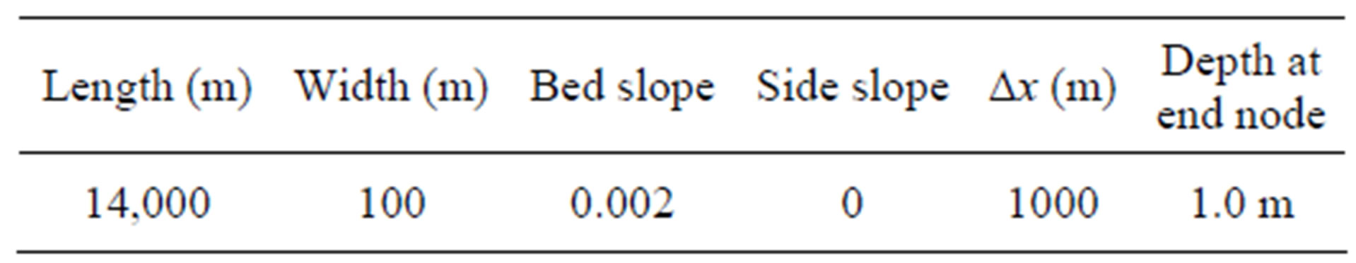
Table 1. Input data for the validation example - -1.
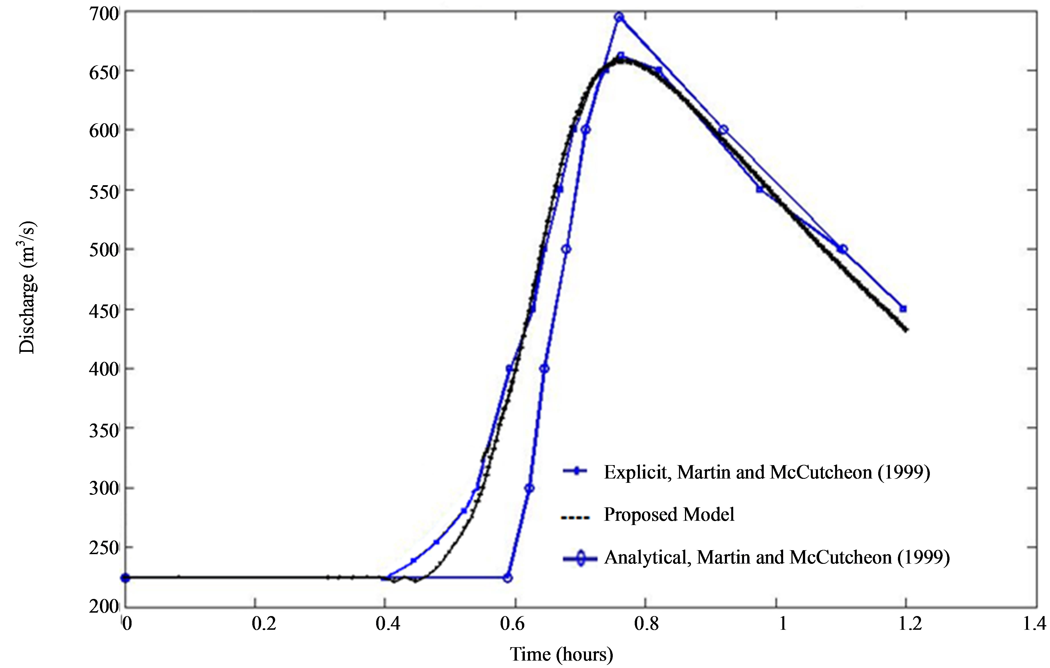
Figure 2. Transient flow simulation profiles at 11th km: Validation Example-1.
downstream boundary. The upstream boundary conditions are given by: DO (0, t) = 8.5 + 3.5cos (2πt) in mg/L, where t = 0 at noon and it is in days. Concentrations of DO all along the channel at time t = 0 are zero. The kinetic reaction constants and solute characteristics are given as k1 = 0.25 /day, kR = 2/day, and DOsat = 9.5 mg/L, Cl = 5.0 mg/(L∙.day). Other input data for flow conditions are presented in Table 2. The simulated variations in DO with distance at 6:00 PM and 6:00 AM after ten days are compared with analytical solutions given by [2122]. This is presented in Figures 3 and 4, respectively. It can be observed from these figures that, as in the case of constant loading, numerically simulated DO variations matched satisfactorily with analytical solutions. Thus it can be concluded that the adapted simulation model can be satisfactorily utilized for predicting water quality response of a river to imposed flow and pollutant loading conditions.
4. Illustrative Application of the Management Model
The management model developed in this study is applicable for the water quality management in tidal rivers subjected to a given pollutant loading. Illustrative appli-
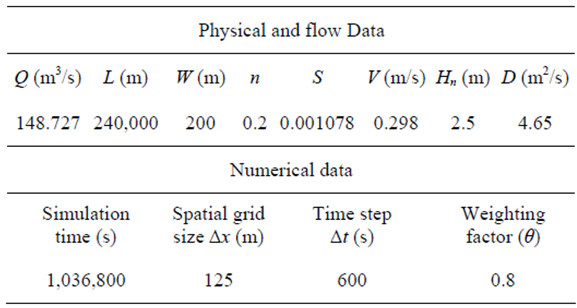
Table 2. Input data for validation example-2 [2122].
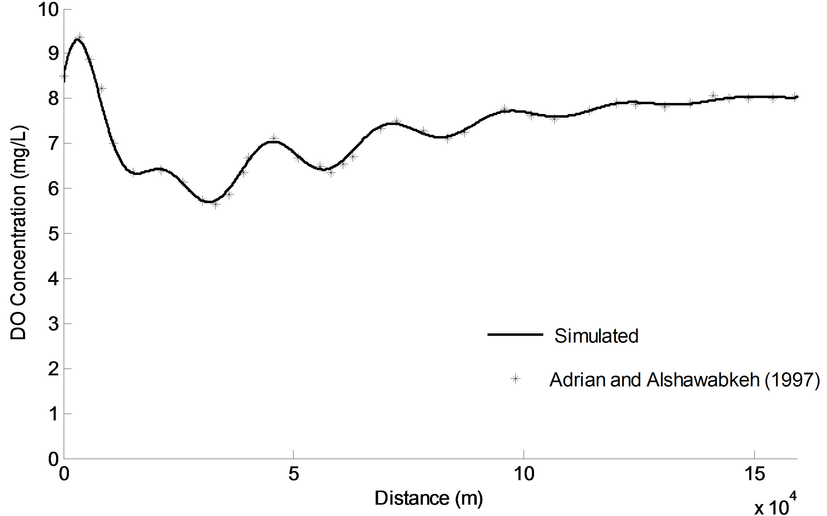
Figure 3. Dissolved Oxygen (DO) profile at 6 PM for Example-3.
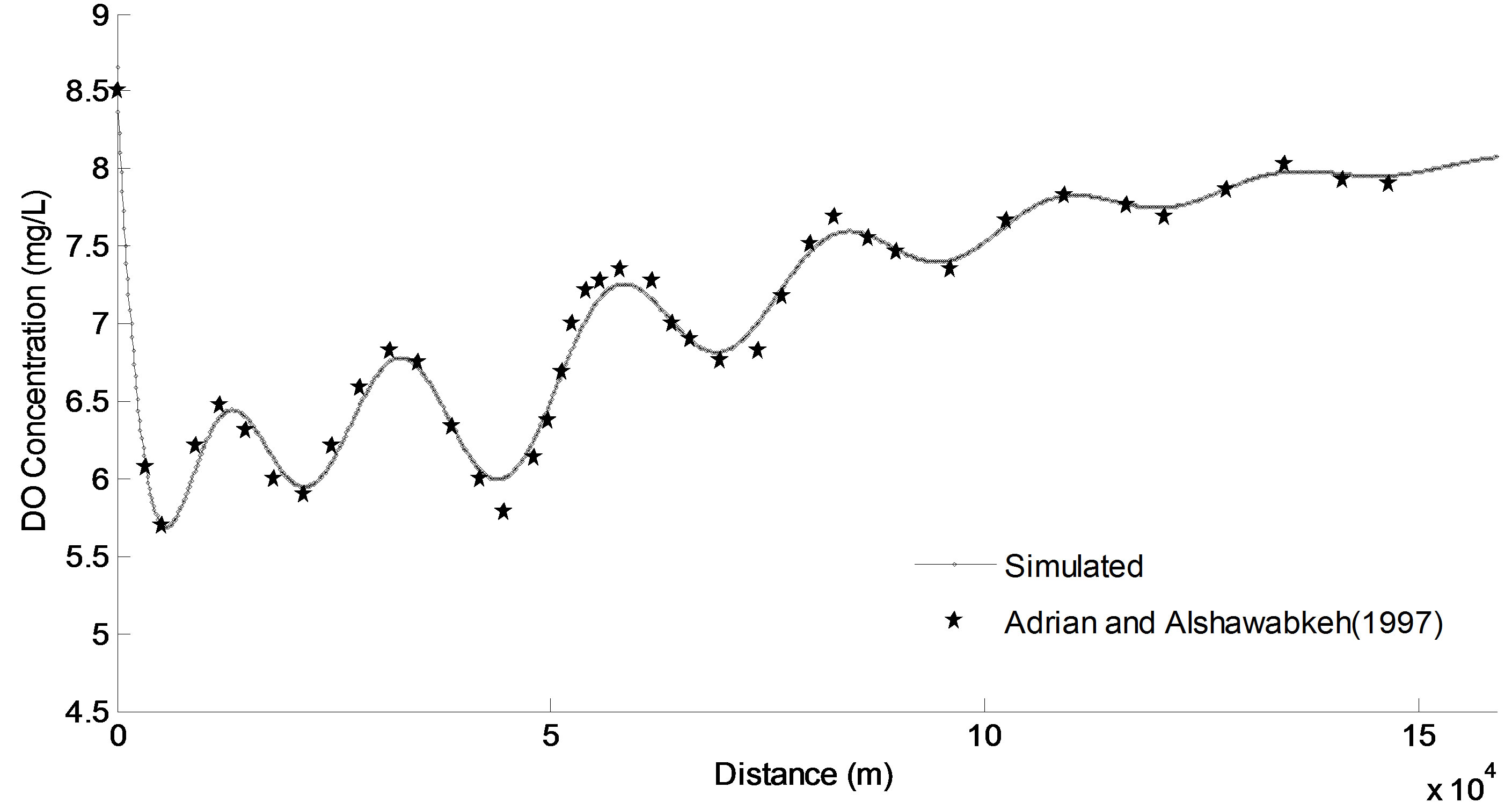
Figure 4. Dissolved Oxygen (DO) profile at 6 AM for Example-3.
cations of management model presented in this study are intended to test the feasibility, applicability and evaluation of the methodology under representative conditions and for the case of Adyar River in Chennai, India. It may be mentioned that discussions presented in this section are subject to the limitations and assumptions in the simulation model.
4.1. Description of the Study AREA
A hypothetical data set representing a tidal channel is used to illustrate various example applications of the proposed management model. The hypothetical system considers a 15 km long channel, with an environmental reservoir at the upstream end, releases, which are used for maintaining the water quality in the river. The geometric and flow data for this illustrative channel are as presented in Table 3. The channel is subjected to a sinusoidal tidal variation at its mouth (downstream end). This channel is subjected to a point pollution loading at a distance of 5.0 km from the upstream end of the river, with the rate of BOD loading ranging from 1500 mg/L to 4500 mg/L at a pollutant discharging rate of 1 m3/s, for different cases. The initial (at t = 0) BOD concentrations along the full stretch of the river are considered to be zero, while the DO concentration is its saturated value (9.2 mg/L). The kinetic reaction constants (kR and k1) and the dispersion coefficients are given as a function of the flow parameters by Equations (9) - -(11).
The illustrative example problem is solved for the case of Adyar River as well. Adyar River originates near the Chembarambakkam Lake in Chengalaputta district, which is about 15 km west of Tambaram near Chennai. It is one of the two rivers, which winds through Chennai (Madras), capital city of Tamil Nadu in South India. It covers about 12.2 km within basin area of Chennai limits. It joins the Bay of Bengal at the Adyar Estuary (13˚°0′47″N, 80˚°16′37″E) Figure 5. Despite the high pollution levels, boating and fishing take place in this river.
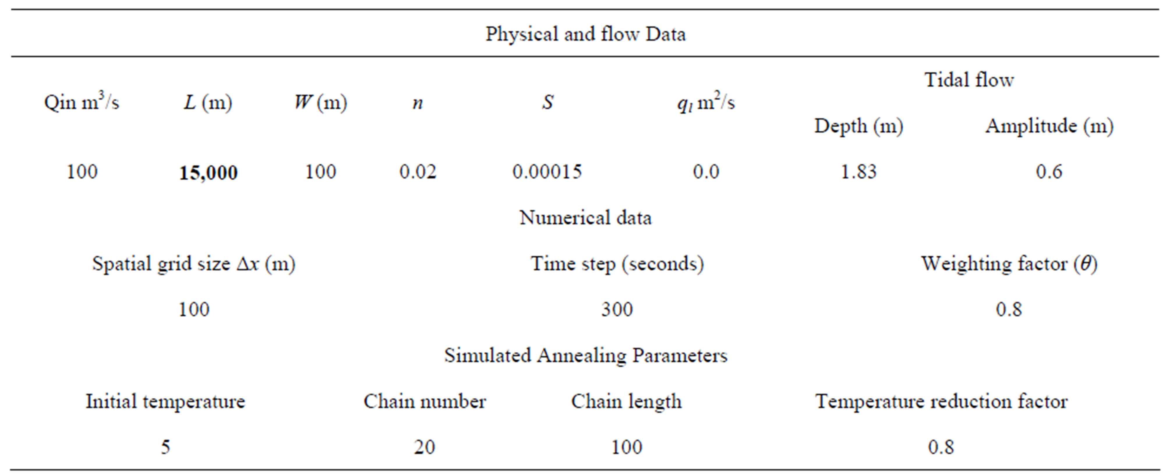
Table 3. Input data to the water quality model in the SA optimization model.
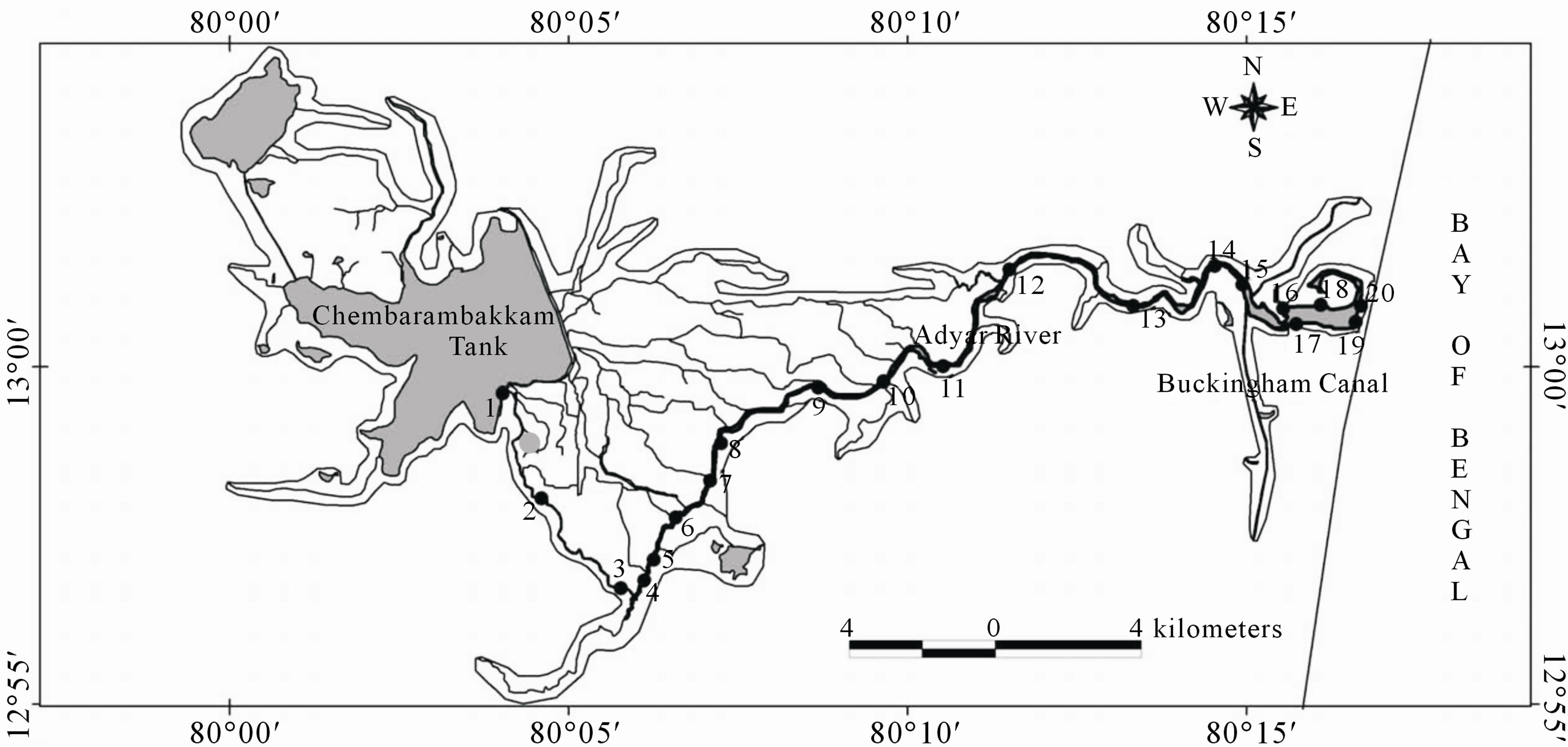
Figure 5. Adyar river map [25].
Initial flow conditions in the channel cannot correspond to steady uniform flow conditions as the river is subjected to tidal variation in all the cases. Therefore, arbitrary flow data is prescribed at all the nodes in the channel at time t = 0, with correct inflow condition at the upstream end. The flow module is then used, along with the prescribed tidal variation at the downstream end, to evolve the flow conditions in the channel for at least three tidal cycles. During these computations, the inflow rate at the upstream end is kept constant. The evolved flow conditions after three tidal cycles are used as initial conditions for subsequent application of the management model in all the cases.
The annealing parameters were specified based on guidelines suggested by [8] and [2223] while applying the simulated annealing optimization algorithm. Extensive numerical experimentation was carried out to choose appropriate values of (1) the initial temperature, (; 2) number of temperature reductions, (; 3) maximum number of iteration within each temperature and (4) the temperature reduction factor. In this work, the initial temperature is 5, the number of temperature reductions is 20, the chain length (number of iteration for each temperature) is 100 and the temperature reduction factor is 0.8. The evolution of the optimization model solution using the SA algorithm for a typical problem is shown in Figure 6. It is assumed that the termination criterion is met if four or more successive temperature reductions did not yield any improvement in the solution. In this work the significance of tidal effect on water quality management in a tidal river is illustrated first by using a hypothetical river system and then the management model is applied to Adyar River in Chennai India.
4.2. Effect of Tidal Flow
To understand the effect of tidal variation on the maintenance of river water quality, twelve runs are made for the hypothetical river system using the proposed simulation-optimization model. The management model is used for determining the minimum constant upstream flow rate that is required to maintain the DO value in the river above a minimum specified value (5.0 mg/L). In each case, the BOD loading rate at the pollution discharge point is kept time invariant, while it ranged from 1500 mg/L to 4500 mg/L for different cases. Numerical experiments are carried out for two different conditions: (1) tidal variation at the downstream end, ; and (2) constant flow depth at the downstream end, in order to illustrate the effect of tidal variation on water quality management.
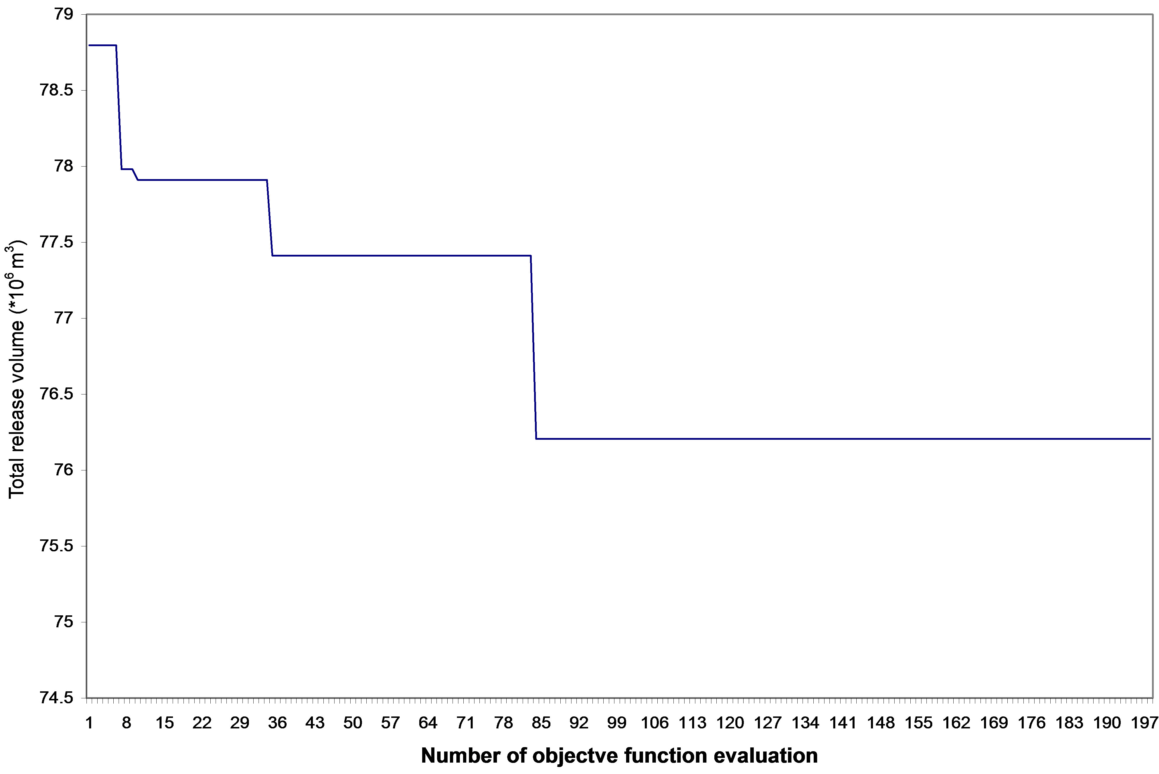
Figure 6. Evolution of the objective function in a typical optimization model solution.
The minimum constant upstream release that is required to maintain the river water quality as a function of pollutant loading rate is presented in Figure 7, for both the cases of constant depth (non-tidal) and tidal boundary conditions at the downstream end. It can be observed from Figure 7, the minimum upstream flow required for water quality maintenance is lesser in the case of a river with tidal boundary as compared to the case of same river with a constant depth downstream boundary condition. The tidal ingress of relatively fresh water from sea during the high tide reduces the need for upstream release for same standard of water quality and pollutant loading scenarios as compared to that for non tidal condition. The reduction in the required minimum upstream release due to tidal effect increases with the pollution loading rate. For the particular case studied here, the reduction in the requirement of minimum in stream flow, ranges from 15% to 19 % for the cases of a pollution loading rate of 1500 mg/L to 4500 mg/L. This reduction in the requirement of water for maintaining the water quality leads to increased availability of water for other purposes such as drinking water supply and irrigation. It can also be observed from Figure 7 that larger upstream releases are required to maintain the in-stream water quality for elevated pollution loading rates, as expected. While only 167 m3/s of water release is sufficient to maintain the water quality for a pollution loading rate of 1500 mg/L, a release of 357 m3/s is required in case of a loading rate of 4500 mg/L. In the case of non tidal boundary condition, the flow rates are 196.4 m3/s and 440.7 m3/s for the loading rates of 1500 mg/L and 4500 mg/L, respectively.
The optimization problem solved in the above cases involves only a single decision variable (single upstream flow rate), and the solutions for these cases can be easily obtained through enumeration. This helps in evaluating the performance of the SA technique used in the management model. It is found in the present study that the solutions determined using the enumeration technique coincided with those obtained using the SA technique for optimization, thus indicating a satisfactory performance of the optimization module of the water quality management model. It may be noted that enumeration technique can be used only for simple cases, and the use of proposed management model with SA technique becomes essential for complex cases, where the release from the upstream environmental reservoir can vary with time.
4.3. Optimal Time Varying Release
Earlier studies on tidal rivers [11] have indicated how the effluent discharge can be varied with time, to match with the tidal cycle, in order to maintain acceptable water quality in tidal water systems. Significantly lower contaminant concentrations in the river were obtained by varying effluent discharge into the river system in accordance with the absolute flow rate. Similarly, for a given time invariant pollutant loading and tidal variation, it may be possible to vary the upstream flow rate with time, with the objective of minimizing the total release volume over a management period, while maintaining the river water quality standards. This is demonstrated in this section by solving the optimization problem wherein a day
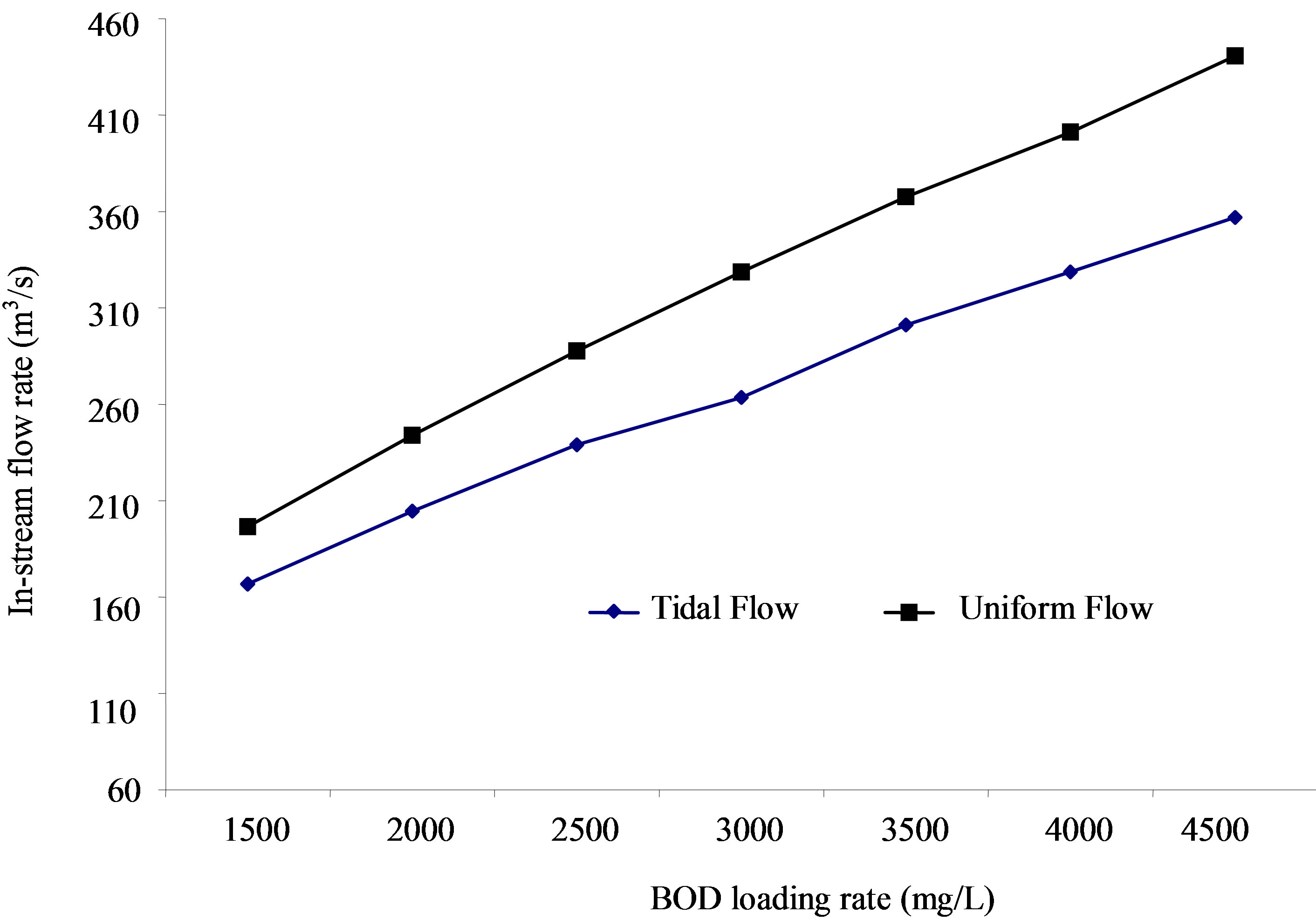
Figure 7. Minimum in stream flow as a function of pollutant loading rate.
is divided into four equal time periods (M = 4; and Tk = 6 hrs for all k = 1 to 4), with upstream flow rate being different during each time period. As mentioned earlier, total management period is three days, with the daily inflow pattern being same on all the three days. Thus, this optimization problem involves four decision variables, Qrel,k, for k = 1 to 4. Other data concerning the channel geometry, tidal variation, and pollutant characteristics are the same as given earlier. Numerical runs for optimal release pattern are carried out for five different pollutant loading rates: 1500, 2000, 2500, 3500 and 4500 mg/L. Table 4 shows the optimal release pattern obtained using the management model developed in this study for both tidal and non tidal flow scenarios. As described in the earlier section, this problem is also solved assuming that the rate of upstream release is constant throughout the day. The total volume of water released from the upstream reservoir to maintain the water quality over a period of three days, obtained for the case of constant upstream release is compared with that obtained for the case of varying upstream release. It can be observed from Figure 8 that water required for maintaining the river water quality can be reduced by temporally varying the upstream releases to match with the tidal variation at the downstream end. For example, it is required to release 78 Mm3 of water in three days in order to keep the DO levels in the river above the minimum value of 5.0 mg/L if the upstream release is kept constant throughout, and the BOD loading rate is 3500 mg/L. On the other hand, it is required to release only 76 Mm3 of water when the upstream releases are varied temporally. The volume of water saved by resorting to time varying release pattern shows an increasing trend as the rate of pollution loading increases (Figure 8). It can also be observed from Table 4 that, as expected, the temporal variation in the optimal rates of upstream release is insignificant when the downstream condition corresponds to a nontidal boundary. Consequently, for the case of non-tidal boundary condition, the difference between optimal total release volumes obtained (1) assuming temporal variation in release rates, ; and (2) assuming constant release rate, is insignificant (Figure 8).
It may be possible to achieve further savings in use of water for dilution by increasing the number of release intervals i.e., by increasing M in the management model. This aspect is evaluated by making five different numerical runs of the management model with M = 1, 2, 4 and 6 and 8, for two pollutant loading rates of 1500 mg/L and 2000 mg/L. Figure 9 shows the optimal upstream release volume obtained as a function of the number of time intervals (in a day) for varying the upstream release. It can be observed from Figure 9 that the total amount of water required for maintaining water quality over the
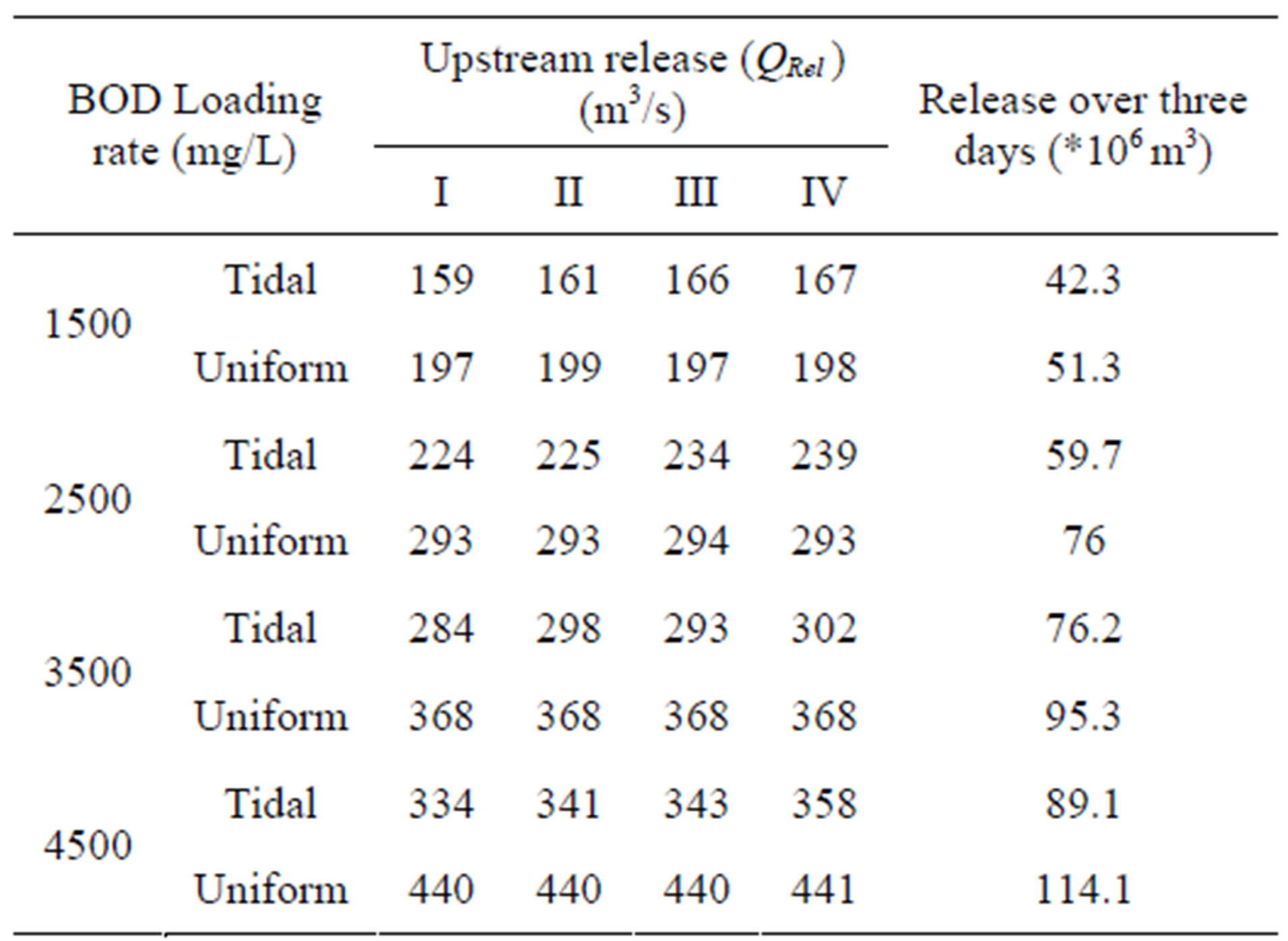
Table 4. Optimal release values under uniform and tidal boundary conditions.

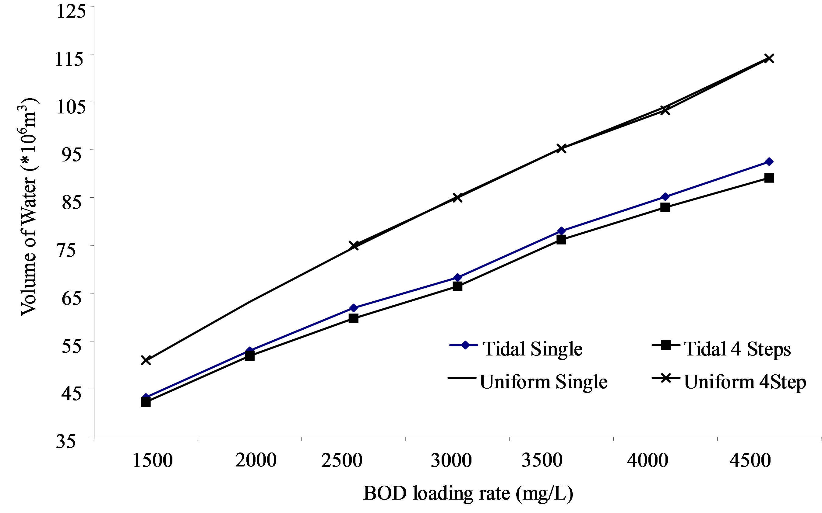
Figure 8. Optimal released over the management period.
management period reduces as the number of release intervals M increases. This indicates that water can be saved by reducing the rate of upstream release more frequently, depending on the tidal level. Higher release rates are required only during the low tide.
In all the cases discussed so far, Tk (duration of time for which a particular rate of release is maintained) is a constant for all k and is equal to 24/M hours. It is tested here whether it is possible to obtain a better optimal solution if Tks are also considered as decision variables. In the example problem illustrated here, it is assumed that the day is divided into four (M = 4) unequal intervals and the rate of release is different during each of these intervals. The number of decision variables is eight in the optimization problem. This problem is solved for two pollutant loading rates of 1500 mg/L and 4500 mg/L, and the results are presented in Table 5. It can be observed from Tables 4 and 5 that there is a further marginal improvement in optimal results i.e. minimization of water required for maintaining the water quality by taking the time interval also as a decision variable.
4.4. Water Quality Management in Adyar River
An attempt is made to use the single objective optimization model for evaluating several alternative strategies for maintaining water quality in Adyar River through optimal release of water from an upstream environmental

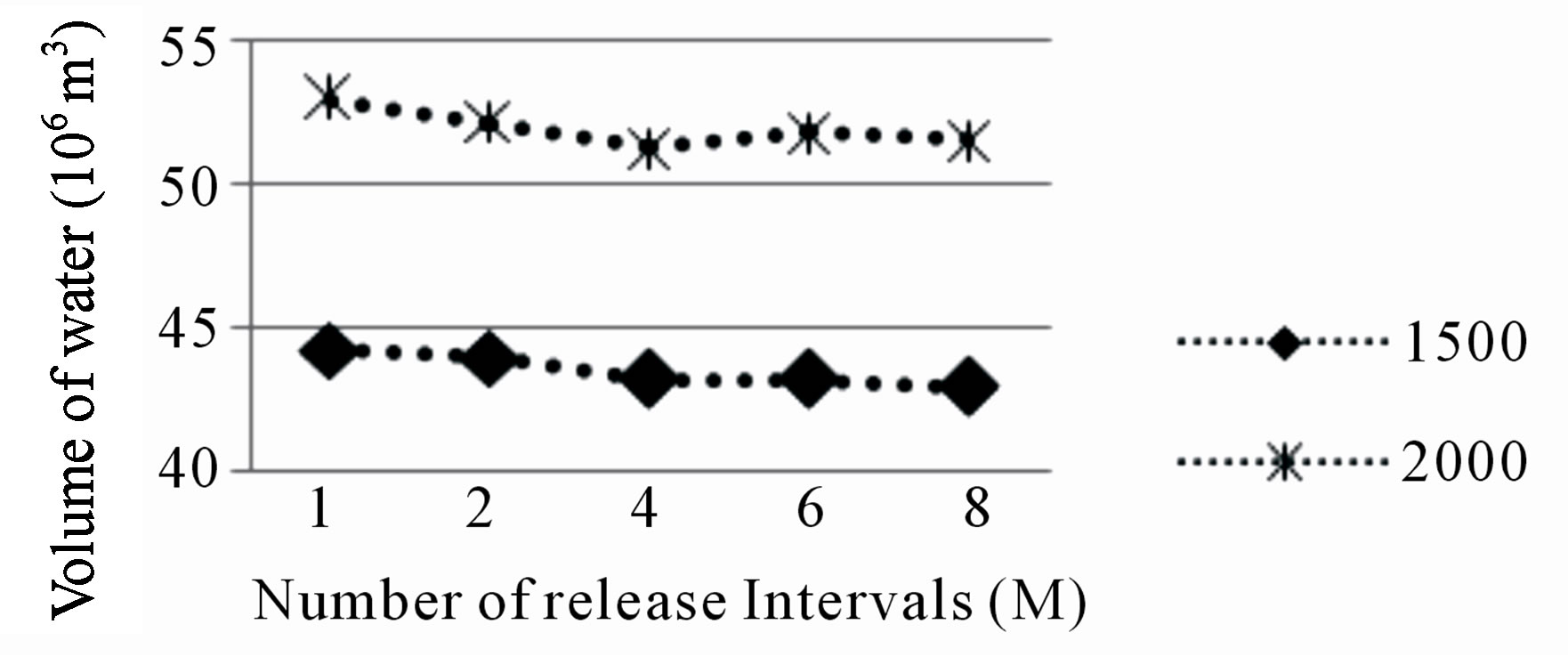
Figure 9. Optimal total release volumes as a function of number of intervals for varying the release rate.
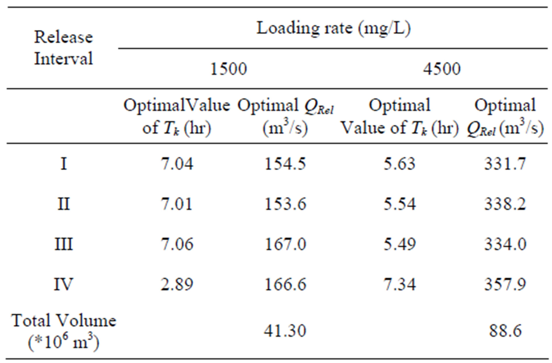
Table 5. Optimal solution with Tk also as decision variables.
reservoir. Although attempts have been made to calibrate the simulation model, the calibration can be considered only partial because complete flow, cross-sectional and depth data are not available. The results presented in this section should be viewed only as planning level results for comparing several strategies to maintain water quality in the Adyar River. The river receives a sizeable quantity of sewage after reaching Nandambakkam near Chennai. The total amount of sewage produced in Adyar river basin is about 96.4 Million Liters per Day (MLD). Out of this 77.0 MLD is treated (from 350 mg/L raw sewage to 10 mg/L after treatment) at Nesapkkam Sewage Treatment Plant (STP) (23 MLD) and Perungudi STP (54 MLD). The remaining 19.4 MLD is supposed to be discharged to the river untreated. On the other hand, based on the average amount of water supply to the basin area (i.e. 135.0 LPCD), the amount of sewage produced in Adyar river basin is expected to be 132.7 MLD. Based on this figure and the total amount of treated sewage (i.e. 77.0 MLD), there is an amount of 55.7 MLD untreated sewage that could make its way to Adyar river. In this work, we considered that, this amount of sewage with the specified BOD concentration of 350 mg/L is released in to the river system at five prominent sewage effluents outlet points (i.e. Chennai bypass, MIOT Hospital, Sidapet near Parsan Nagar, Kotturpuram bridge and green way road) which are located at 10, 14, 19, 20 and 25 km from upstream end. The sewage after treatment is released in the lower river catchment near Kasi Bridge in the industrial area.
The river is almost stagnant except during the rainy season. The river has varying depth with approximately 0.75 m in its upper reaches and 0.5 m in its lower reaches. It discharges about 190 to 940 million m3 water annually to the Bay of Bengal [2324], which is –-6.02 m3/s to –-29.8 m3/s. The peak discharge is about, 200 m3/s, which is 7 to 33 times more than the annual average during the North East monsoon season between Septembers to December. The river is sub divided into three segments based on their overall concentration ranges of dissolved gases and inorganic nutrients (Table 6). In this work we considered lower basin, where the BOD loading is high and the DO is worst. During low flow periods (February and August) the development of a sand bar across the mouth of the estuary due to monsoon-driven long shore drift typically reduces the tidal range from –-0.6 m to –-0.2 m [2425]. This explains that the dissolved O2 in the lower catchments and estuary must be replenished mainly via air–-sea gas exchange and the importance of the tidal flow.
4.5. Optimal Upstream Reservoir Release
Several management strategies are suggested to maintain the water quality of the river to a minimum DO standard
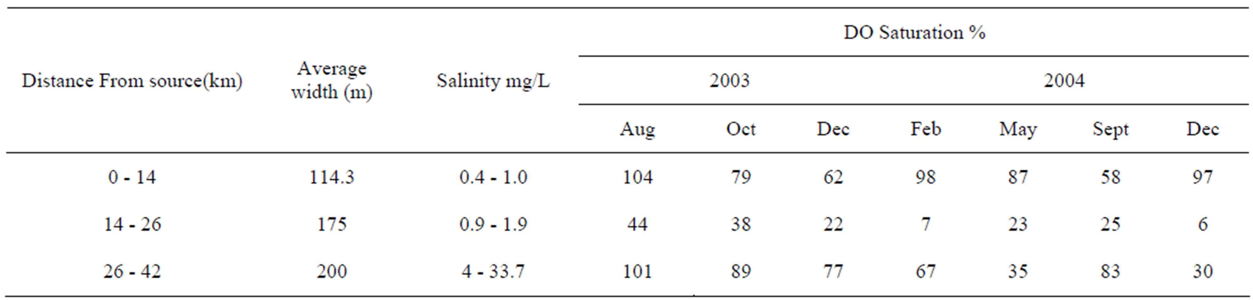
Table 6. Mean concentrations of dissolved oxygen data, salinity in the three Adyar river segments [25].
of 5 mg/L, assuming the creation of an upstream reservoir in the future, and based on the total estimated sewage effluent discharged into the river and the capacity of existing treatment plant. The first option is to operate the existing sewage treatment as it is now and use an upstream reservoir release for dilution. The second is to treat the entire sewage discharged in to the river system to 50%, 75% and 97% removal of BOD, and then use upstream reservoir releases. In these options, it is assumed that a constant rate of upstream release is maintained, and the interest is to determine the minimum rate of upstream release that is required. The respective optimal upstream reservoir releases to meet a DO standard of 5 mg/L in the Adyar River under a given treatment level of the sewage effluent are presented in Figure 10. In the first scenario, an upstream release of 116 m3/s is required to maintain the river water quality, compared to the existing 10 m3/s lean flow rate. This means an extra 106 m3/s of release from upstream reservoir needs to be obtained. On the other hand, if all the sewage is treated for 97% of BOD removal, one would require only 82 m3/s of in-- stream flow. If we reduce the effluent concentration to its 75% and 50% of raw strength, we need 78 m3/s and 84 m3/s extra upstream environmental releases to maintain the stream water quality to 5 mg/L, respectively. The simulated DO profile plots for the respective cases of treatment are presented in Figure 11. The DO levels in all the cases are above the minimum DO standard specified to be maintained in this work.

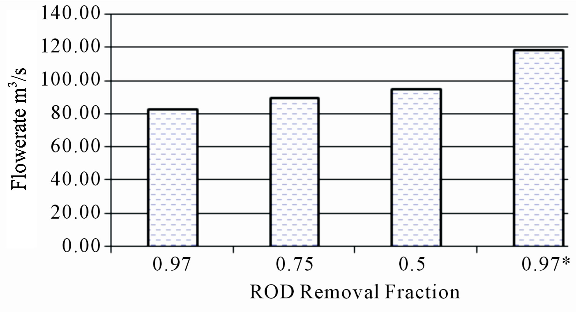
Figure 10. Upstream reservoir releases on Adyar River.
5. Summary
In this study, a simulation-optimization model is proposed for the management of water quality in a tidal river using releases of water from an upstream environmental reservoir. In the proposed management model, a complete hydrodynamic model for transport of BOD and DO in a tidal river is linked to Simulated Annealing (SA) algorithm for optimization in a simulation-optimization framework. The boundary conditions correspond to a temporally varying water releases at upstream end and temporally varying water level at the downstream end. The performance of the proposed methodology is evaluated for an illustrative river and for Adyar River in Chennai, India. Application of the management model has shown that significantly less amount of upstream water release is required to maintain the DO standard in a tidal river as compared to that in a corresponding non-tidal river. It is demonstrated that it is possible to reduce the amount of water released to maintain the water quality by resorting to a time varying release policy, wherein the rate of upstream release is different during different time durations, in accordance with the tidal levels. It is found that more savings in water can be achieved by allowing for more changes in the rate of upstream release during a day. The proposed model will be helpful in arriving at best water release policy for maintaining water quality in tidal rivers for given tidal variation and pollutant loading. The results presented here are meant only for illustrative purpose. They do not establish the range of validity of the management model.
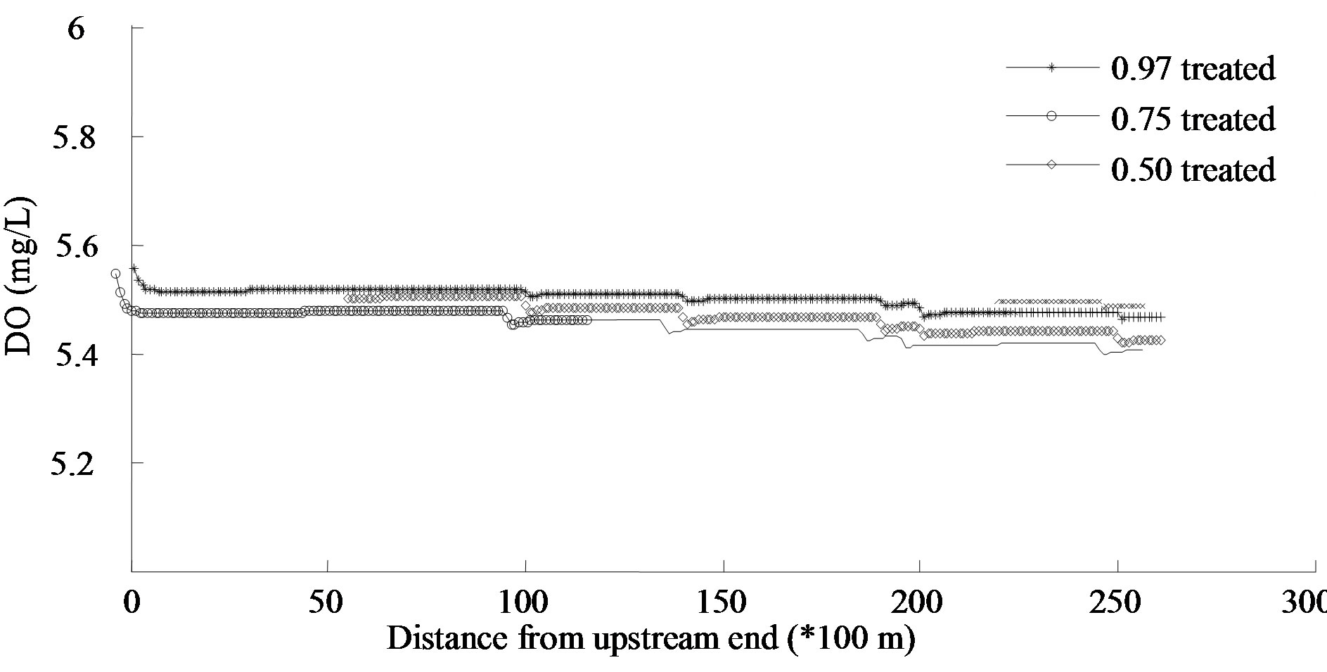
Figure 11. Simulated DO profiles for given treatment levels.
Also, the applicability of the proposed methodology is limited by the assumptions on which the simulator is based. The simulation model should be modified to take into account the effect of spatially and temporally varying salinity on the mixing process for the contaminant.
REFERENCES
- E. D. Ongley, “Water Quality Management: Design, Financing and Sustainability Considerations-II,” World Bank’s Water Week Conference: Towards a Strategy for Managing Water Quality, Washington, D.C. , 3-4 April 2000.
- A. Elshorbagy, and L. Ormsbee, “Object-Oriented Modeling Approach to Surface Water Quality Management,” Environmental Modeling & Software, Vol. 21, No. 5, 2006, pp. 689-698. doi:10.1016/j.envsoft.2005.02.001
- L. C. Brown, and T. O. J. R. Barnwell, “The Enhanced Stream Water Quality Models QUAL2E and QUAL2EUNCASP Documentation Manual,” US Environmental Protection Agency, Athens, GA, 1987.
- S. R. M. Yandamuri, S. M. Bhallamudi and K. Srinivasan, “Non-Uniform Flow Effect on Optimal Waste Load Allocation in Rivers,” Water Resources Management, Springer, Vol. 20, 2006, pp. 509–-530.
- A. Dhar, and B. Datta, “Optimal Operation of Reservoirs for Downstream Water Quality Control Using Linked Simulation Optimization,” Journal of Hydraulic Process, Vol. 22, No. 6, 2008, pp. 842–-853. doi:10.1002/hyp.6651
- K. I. Mumme, “Cyclic Control of Water Quality in Tidal River Segment,” Pergamon press Ltd. Automatica, Vol. 15, 1979, pp. 47-57.
- C. Fan, W. S. Wang, and M. C. Liao, “Impact of Tidal Effects on Water Quality Simulation of Rivers Running through Urban Area a Case Study in North Taiwan,” International Society of Environmental Information ScienceISEIS, Vol. 5, 2007, pp. 409-414.
- R. A. Maryott, “Optimal Groundwater Management Simulated Annealing,” Water Resources Research, Vol. 27, No. 10, 1991, pp. 2493–-2508. doi:10.1029/91WR01468
- A. Vasan, and K. S. Raju, “Comparative Analysis of Simulated Annealing, Simulated Quenching and Genetic Algorithms for Optimal Reservoir Operation,” Applied Soft Computing, Vol. 9, No. 1, 2009, pp. 274–-281. doi:10.1016/j.asoc.2007.09.002
- M. H. Chaudhry, “Open Channel Flow. ,” 2nd Edition, New Jersey: Prentice Hall, New Jersey, 2008. doi:10.1007/978-0-387-68648-6
- J. H. Bikangaga, and V. Nassehi, “Application of Computer Modeling Techniques to the Determination of Optimum Effluent Discharge Policies in Tidal Water System,” Water Resources, Elsevier Science Ltd, Vol. 29, No. 10, 1995, pp. 2367- 2375.
- R. L. Runkel, “Toward a Transport-Based Analysis of Nutrient Spiraling and Uptake in Streams,” Limnology and Oceanography: MethodsLimnol Oceanogr: Methods, US, Vol. 5, 2007, pp. 50–-62
- J. D. Wang and K. L. Vassiliki, “Circulation on the Continental Shelf of the Southeastern United States Part II: Model Development and Application to a Tidal Flow,” Journal of Physical OceanographyAmerican Metrological Society, 1984., Vol. 14, No. 6, 1984, pp. 1013-1021.
- H. B. Fischer, E. J. List, R. C. Y. Koh, J. Imberger, and N. H. Brooks, “Mixing in Inland and Coastal Waters,” Academic, New York, 1979.
- W. Seo, and T. S. Cheong, “Predicting Longitudinal Dispersion Coefficient in Natural Streams,” Journal of Hydraulic Eng., Vol. 124, No. 1, 1998, pp. 25-33.
- S. C. Chapra and R. P. Canale “Numerical Methods for Engineers,” McGraw Hill, 5th Ed., ition, McGraw Hill, New York, 1988.
- W. C. Liu, S. Y. Liu, M. H. Hsu, and A. Y. Kuo, “Water Quality Modeling to Determine Minimum in Stream Flow for Fish Survival in Tidal Rivers,” Journal of Environmental Management, Vol.76, No. 4, 2005, pp. 293-308. doi:10.1016/j.jenvman.2005.02.005
- S. C. D. Kirkpatrick, and G. M. P. Vecchi, “Optimization by Simulated Annealing,” Science New Series, Vol. 220, No. 4598, 1983, pp. 671–-680.
- J. L. Martin, and S. C. MaCutcheon, “Hydrodynamics and Transport for Water Quality Modeling,” CRC Press, Inc., New York, 1999.
- R. Dresnack, and W. E. Dobbins, “Numerical Analysis of BOD and DO Profiles,” Journal of Sanitary Engineering Division (Proceeding of the ASCE)Journal Sanit. Eng. Div. Am. Soc. Civ. Eng., Vol. 94, No. 5, 1968, pp. 789-808.
- D. D. Adrian, and A. N. Alshawabkeh, “Analytical Dissolved Oxygen Models for Sinusoidally Varying BOD,” Journal of Hydrologic Eng. ineering, Vol. 2, No. 4, 1997, pp. 180-187. doi:10.1061/(ASCE)1084-0699(1997)2:4(180)
- O. Onyejekwe, and S. Toolsi, “Certain Aspects of Green Element Computational Model for BOD-DO Interaction.,” Advances in Water Resources, Vol. 24, No. 2, 2001, pp. 125–-131. doi:10.1016/S0309-1708(00)00048-8
- S. V. N. Rao, S. M. Bhallamudi, B. S. Thandaveswara, and V. Srinivasulu, “Planning Groundwater Development in Coastal Deltas with Paleo Channels,” Water Resources Management, Vol. 19, No. 5, 2004, pp. 625– -639. doi:10.1007/s11269-005-5604-y
- K. Krishnaveni, and V. Gowri, “Application of GIS in the Study of Mass Transport of Pollutants by Adyar and Cooum Rivers in Chennai (Madras), Tamil Nadu,” Environmental Monitoring and Assessment, Vol. 138, No. 1-3, 2008, pp. 41–-47. doi:10.1007/s10661-007-9789-9
- A. N. Rajkumar, R. Ramesh, R. Purvaja, J. Barnes and R. C. Upstill-Goddard, “Methane and Nitrous Oxide Fluxes in the Polluted Adyar River and Estuary, SE India,” Marine Pollution Bulletin, Vol. 56, No. 12, 2008, pp. 2043- 2051.