Influence of Vertical Resolution on the Validation of Atmospheric Chemistry Instruments

doi:10.4236/acs.2011.13011

Paper Menu >>

Journal Menu >>

Atmospheric and Climate Sciences, 2011, 1, 95-99

doi:10.4236/acs.2011.13011 Published Online July 2011 (http://www.scirp.org/journal/acs)

Influence of Vertical Resolution on the Validation of

Atmospheric Chemistry Instruments

Guochang Zhang

Department of Physi cs a nd In f orm ati o n E ngineering, Shangqiu Normal University, Shangqiu, China

E-mail: [email protected]

Received March 5, 2011; revised April 22, 2011; accepted M ay 1, 2011

Abstract

A large number of validation campaigns for atmospheric chemistry instruments are being carried out and

more such studies will be performed in the future. The aims of validation are to confirm the accuracy and

precision of the measurement of a new instrument. There are many factors that may deteriorate the validation

results and one of them is the vertical resolution of instruments when using the profiles intercomparison ap-

proach. The influence from the vertical resolution can be eliminated by using the averaging kernel method

but it is necessary to find the conditions for using the method. This study simulated the influence of vertical

resolution for a certain curvature. The results show that both the curvature of a profile and the difference of

vertical resolution between two instruments have positive correlation with the differences between their

measurements. The quantitative estimations of influence for some practical vertical resolutions were ob-

tained. The combined error of two instruments was defined as the criteria to judge the significance of influ-

ence. A case study based on the simulated results was demonstrated to show when the influence from the

vertical resolution should be considered and when such influence can be omitted in order to avoid some un-

necessary works in validation.

Keywords: Simulation, Validation, Vertical Resolution, Atmospheric Chemistry Instrument

1. Introduction

Limb-scanning remote-sounding atmospheric chemistry in-

struments onboard satellit es are widely used t o measure

atmospheric parameters like the density of gases, tempera-

ture and pressure at different altitudes, thus forming pro-

files of par ameters. For the validation of a new remote

sounder, it is necessary to compare its measurements with

the observations of other proved instruments at the same

time and location. There are many factors that can deterio-

rate the validation results, for example, measuring different

air masses because of atmospheric fluidity, the che mical

reaction in the atmosphere, the different characteristics of

instruments like the vertical and horizontal resolution, etc.

[1,2]. The vertical resolution should be especially con-

cerned during the validation for limb-scan remote sounders

which usually present their output data with profile form of

atmospheric parameters. Figure 1 shows an intercompari-

son of temperature profiles during the validation for MI-

PAS/ENVISAT, Michelson Interferometer for Pas sive

Atmospheric Sounding aboard the Environmental Satellite

of European Space Agency [3,4] (this instrument is named

MIPAS-E hereafter) by using the data from MIPAS-B — a

remote sounder that is similar to MIPAS-E but aboard a

large Balloon [5-7]. Both instruments adopted

limb-sounding geometry and can measure tens of atmos-

pheric parameters profiles like pressure and temperature

profiles, mixing volume ratio profiles of O3, H2O, HNO3,

N2O, CH4 and NO2 etc. within a short period of time. In the

figure, the right panel gives the temperature profile of

MIPAS-E with vertical resolution 3 km, the profile of the

same parameter from MIPAS-B but with vertical resolution

1 km which is the nominal resolution of the instrument. An

additional retrieved temperature profile from MIPAS-B

with vertical resolution 3 km was also presented. The left

panel gives the differences of profiles between MIPAS-E

and MIPAS-B with vertical resolution 3 km, 1 km and its

smoothed profile (details in section 3.3), respectively. The

agreements between the MIPAS-E and MIPAS-B profiles

are generally good in the whole altitude range of compari-

son. However, in the range of 169 - 126 hPa (11 - 15 km ),

the differences are obviously larger when using the MI-

PAS-B profile with vertical resolution 1 km than the dif-

ferences when using another MIPAS-B profile with verti-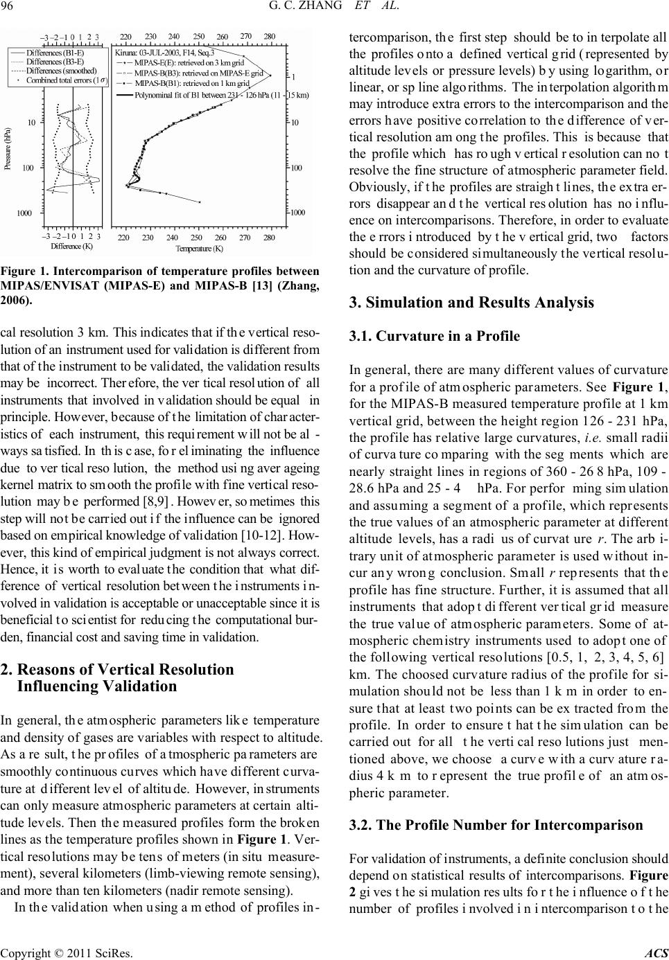

96 G. C. ZHANG ET AL.

Figure 1. Intercomparison of temperature profiles between

MIPAS/ENVISAT (MIPAS-E) and MIPAS-B [13] (Zhang,

2006).

cal resolution 3 km. This indicates that if the vertical reso-

lution of an instrument used for validation is different from

that of the instrument to be validated, the validation results

may be incorrect. Therefore, the vertical resolution of all

instruments that involved in validation should be equal in

principle. However, because of the limitation of character-

istics of each instrument, this requirement will not be al-

ways satisfied. In this case, for eliminating the influence

due to vertical resolution, the method using averageing

kernel matrix to smooth the profile with fine vertical reso-

lution may be performed [8,9]. However, sometimes this

step will not be carried out if the influence can be ignored

based on empirical knowledge of validation [10-12]. How-

ever, this kind of empirical judgment is not always correct.

Hence, it is worth to evaluate the condition that what dif-

ference of vertical resolution between the instruments in-

volved in validation is acceptable or unacceptable since it is

beneficial to scientist for reducing the computational bur-

den, financial cost and saving time in validation.

2. Reasons of Vertical Resolution

Influencing Validation

In general, the atmospheric parameters like temperature

and density of gases are variables with respect to altitude.

As a result, the profiles of atmospheric parameters are

smoothly continuous curves which have different curva-

ture at different level of altitude. However, instruments

can only measure atmospheric parameters at certain alti-

tude levels. Then the measured profiles form the broken

lines as the temperature profiles shown in Figure 1. Ver-

tical resolutions may be tens of meters (in situ measure-

ment), several kilometers (limb-viewing remote sensing),

and more than ten kilometers (nadir remote sensing).

In the validation when using a method of profiles in-

tercomparison, the first step should be to interpolate all

the profiles onto a defined vertical grid (represented by

altitude levels or pressure levels) by using logarithm, or

linear, or spline algorithms. The interpolation algorithm

may introduce extra errors to the intercomparison and the

errors have positive correlation to the difference of ver-

tical resolution among the profiles. This is because that

the profile which has rough vertical resolution can not

resolve the fine structure of atmospheric parameter field.

Obviously, if the profiles are straight lines, the extra er-

rors disappear and the vertical resolution has no influ-

ence on intercomparisons. Therefore, in order to evaluate

the errors introduced by the vertical grid, two factors

should be considered simultaneously the vertical resolu-

tion and the curvature of profile.

3. Simulation and Results Analysis

3.1. Curvature in a Profile

In general, there are many different values of curvature

for a profile of atmospheric parameters. See Figure 1,

for the MIPAS-B measured temperature profile at 1 km

vertical grid, between the height region 126 - 231 hPa,

the profile has relative large curvatures, i.e. small radii

of curvature comparing with the segments which are

nearly straight lines in regions of 360 - 268 hPa, 109 -

28.6 hPa and 25 - 4 hPa. For performing simulation

and assuming a segment of a profile, which represents

the true values of an atmospheric parameter at different

altitude levels, has a radius of curvature r. The arbi-

trary unit of atmospheric parameter is used without in-

cur any wrong conclusion. Small r represents that the

profile has fine structure. Further, it is assumed that all

instruments that adopt different vertical grid measure

the true value of atmospheric parameters. Some of at-

mospheric chemistry instruments used to adopt one of

the following vertical resolutions [0.5, 1, 2, 3, 4, 5, 6]

km. The choosed curvature radius of the profile for si-

mulation should not be less than 1 km in order to en-

sure that at least two points can be extracted from the

profile. In order to ensure that the simulation can be

carried out for all the vertical resolutions just men-

tioned above, we choose a curve with a curvature ra-

dius 4 km to represent the true profile of an atmos-

pheric parameter.

3.2. The Profile Number for Intercomparison

For validation of instruments, a definite conclusion should

depend on statistical results of intercomparisons. Figure

2 gives the simulation results for the influence of the

number of profiles involved in intercomparison to the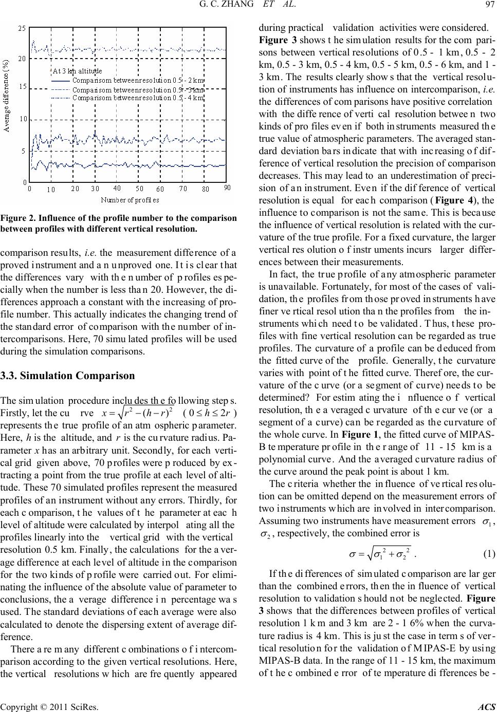

G. C. ZHANG ET AL.

Figure 2. Influence of the profile number to the comparison

between pr ofiles w ith different vertical resolu t ion.

comparison results, i.e. the measurement difference of a

proved instrument and an unproved one. It is clear that

the differences vary with the number of profiles espe-

cially when the number is less than 20. However, the di-

fferences approach a constant with the increasing of pro-

file number. This actually indicates the changing trend of

the standard error of comparison with the number of in-

tercomparisons. Here, 70 simulated profiles will be used

during the simulation comparisons.

3.3. Simulation Comparison

The simulation procedure includes the following steps.

Firstly, let the curve 22

()

rhr (02hr



)

represents the true profile of an atm ospheric parameter.

Here, h is the altitude, and r is the curvature radius. Pa-

rameter x has an arbitrary unit. Secondly, for each verti-

cal grid given above, 70 profiles were produced by ex-

tracting a point from the true profile at each level of alti-

tude. These 70 simulated profiles represent the measured

profiles of an instrument without any errors. Thirdly, for

each comparison, the values of t he parameter at eac h

level of altitude were calculated by interpolating all the

profiles linearly into the vertical grid with the vertical

resolution 0.5 km. Finally, the calculations for the aver-

age difference at each level of altitude in the comparison

for the two kinds of profile were carried out. For elimi-

nating the influence of the absolute value of parameter to

conclusions, the a verage difference in percentage was

used. The standard deviations of each average were also

calculated to denote the dispersing extent of average dif-

ference.

There are many different combinations of intercom-

parison according to the given vertical resolutions. Here,

the vertical resolutions which are frequently appeared

during practical validation activities were considered.

Figure 3 shows the simulation results for the compari-

sons between vertical resolutions of 0.5 - 1 km, 0.5 - 2

km, 0.5 - 3 km, 0.5 - 4 km, 0.5 - 5 km, 0.5 - 6 km, and 1 -

3 km. The results clearly shows that the vertical resolu-

tion of instruments has influence on intercomparison, i.e.

the differences of comparisons have positive correlation

with the difference of vertical resolution between two

kinds of profiles even if both instruments measured the

true value of atmospheric parameters. The averaged stan-

dard deviation bars indicate that with increasing of dif-

ference of vertical resolution the precision of comparison

decreases. This may lead to an underestimation of preci-

sion of an instrument. Even if the difference of vertical

resolution is equal for each comparison (Figure 4), the

influence to comparison is not the same. This is because

the influence of vertical resolution is related with the cur-

vature of the true profile. For a fixed curvature, the larger

vertical resolution of instruments incurs larger differ-

ences between their measurements.

In fact, the true profile of any atmospheric parameter

is unavailable. Fortunately, for most of the cases of vali-

dation, the profiles from those proved instruments have

finer vertical resolution than the profiles from the in-

struments which need to be validated. Thus, these pro-

files with fine vertical resolution can be regarded as true

profiles. The curvature of a profile can be deduced from

the fitted curve of the profile. Generally, the curvature

varies with point of the fitted curve. Therefore, the cur-

vature of the curve (or a segment of curve) needs to be

determined? For estimating the influence of vertical

resolution, the averaged curvature of the curve (or a

segment of a curve) can be regarded as the curvature of

the whole curve. In Figure 1, the fitted curve of MIPAS-

B temperature profile in the range of 11 - 15 km is a

polynomial curve. And the averaged curvature radius of

the curve around the peak point is about 1 km.

The criteria whether the influence of vertical resolu-

tion can be omitted depend on the measurement errors of

two instruments which are involved in intercomparison.

Assuming two instruments have measurement errors 1



, respectively, the combined error is







. (1)

If the differences of simulated comparison are larger

than the combined errors, then the influence of vertical

resolution to validation should not be neglected. Figure

3 shows that the differences between profiles of vertical

resolution 1 km and 3 km are 2 - 16% when the curva-

ture radius is 4 km. This is just the case in terms of ver-

tical resolution for the validation of MIPAS-E by using

MIPAS-B data. In the range of 11 - 15 km, the maximum

of the combined error of temperature differences be-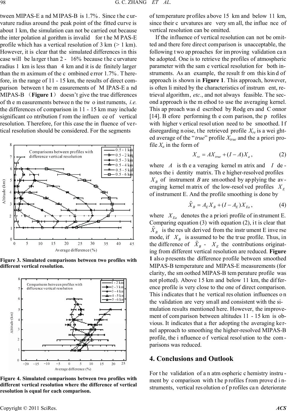

98 G. C. ZHANG ET AL.

tween MIPAS-E and MIPAS-B is 1.7%. Since the cur-

vature radius around the peak point of the fitted curve is

about 1 km, the simulation can not be carried out because

the interpolation algorithm is invalid for the MPAS-E

profile which has a vertical resolution of 3 km (> 1 km).

However, it is clear that the simulated differences in this

case will be larger than 2 - 16% because the curvature

radius 1 km is less than 4 km and it is definitely larger

than the maximum of the combined error 1.7%. There-

fore, in the range of 11 - 15 km, the results of direct com-

parison between the measurements of MIPAS-E and

MIPAS-B （Figure 1） doesn’t give the true differences

of the measurements between the two instruments, i.e.

the differences of comparison in 11 - 15 km may include

significant contribution from the influen ce of vertical

resolution. Therefore, for this case the influence of ver-

tical resolution should be considered. For the segments

Figure 3. Simulated comparisons between two profiles with

different vertical resolution.

Figure 4. Simulated comparisons between two profiles with

different vertical resolution where the difference of vertical

resolution is equ a l for each comparison.

of temperature profiles above 15 km and below 11 km,

since their curvatures are very small, the influence of

vertical resolution can be omitted.

If the influence of vertical resolution can not be omit-

ted and therefore direct comparison is unacceptable, the

following two approaches for improving validation can

be adopted. One is to retrieve the profiles of atmospheric

parameter with the sam e vertical resolution for both in-

struments. As an example, the result from this kind of

approach is shown in Figure 1. This approach, however,

is often limited by the characteristics of instrument, re-

trieval algorithm, etc., and not always feasible. The sec-

ond approach is the method to use the averaging kernel.

This approach was d escribed by Rodgers and Connor

[14]. Before performing the comparison, the profiles

with higher vertical resolution need to be smoothed. If

disregarding noise, the retrieved profile Xre is a weight-

ed average of the “true” profile Xtrue and the a priori pro-

file Xa in the form of

()

re truea

AXIA X



 , (2)

where

is the averaging kernel matrix and

de-

notes the identity matrix. The higher-resolved profiles

of instrument B are smoothed by applying the av-

eraging kernel matrix of the low-resolved profiles

of instrument E. And the profile smoothing is done by

()

EBE Ea

AXIA X

, (4)

where

denotes the a priori profile of instrument E.

Comparing equation (3) with equation (2), it is clear that

 is the result derived from the instrument E inverse

mode, if

is assumed to be the true profile. Thus, in

the difference of

 -

the contributions originat-

ing from different vertical resolution are reduced. Figure

1 also presents the difference profile between smoothed

MIPAS-B temperature and MIPAS-E measurements (for

clarity, the smoothed MIPAS-B temperature profile was

not plotted). Above 15 km and below 11 km, the differ-

ence profile is very close to the one of direct comparison.

This indicates that the vertical resolution influences on

the validation are very small and consistent with the si-

mulation results mentioned here. However, the improve-

ment of comparison between altitudes 11 - 15 km is ob-

vious. It indicates that a fter adopting the averaging ker-

nel approach to smoothing the higher-resolved MIPAS-B

profile, the influence of vertical resolution to the com-

parisons was reduced.

4. Conclusions and Outlook

For the validation of an atmospheric chemistry instru-

ment by comparison with the profiles from proved in-

struments, vertical resolution of profiles can deteriorate

G. C. ZHANG ET AL.

the validation results. The quantitative simulation results

show the extent of deterioration due to the difference of

vertical resolution between the profiles for comparison

for a certain c urvature of profile. The results also show

that when the difference of vertical resolution is equal for

each pair of comparison, the larger vertical resolutions

have more influence on comparison for a given curvature.

The influence of vertical resolution on a validation has to

be considered if its caused difference is beyond the com-

bined errors of two instruments. In general, this kind of

influence can be eliminated or reduced by using the av-

eraging kernel of profile with rough vertical resolution to

smooth the profile with fine vertical resolution.

Since the number of validation activities will increase

in the future, it is useful to simulate the influence of ver-

tical resolution on validation for different combinations

of vertical resolution and different curvatures of profile.

Our next aim is to establish a database based on the

complete simulation results. The database will be freely

accessible for all scientists engaging in validation.

6. References

[1] C. D. Rodgers, “Inverse Methods for Atmospheric

Sounding: Theory and Practice,” World Scientific Press,

Singapore, 2000. doi:10.1142/9789812813718

[2] T. von Clarmann, “Validation of Remotely Sensed Pro-

files of Atmospheric State Variables: Strategies and Ter-

minology,” Atmospheric Chemistry and Physics, Vol. 6,

2006, pp. 4311-4320. doi:10.5194/acp-6-4311-2006

[3] H. Fischer and H. Oelhaf, “Remote Sensing of Vertical

Profiles of Atmospheric Trace Constituents with Mipas

Limb-Emission Spectrometers,” Applied Optics, Vol. 35,

No. 16, 1996, pp. 2787-2796. doi:10.1364/AO.35.002787

[4] H. Fischer, M, Birk, C. Blom, et al, “MIPAS: An Instru-

ment for Atmospheric and Climate Research,” Atmospheric

Chemistry and Phys ics, Vol. 8, 2008, pp. 2151-2188.

doi:10.5194/acp-8-2151-2008

[5] F. Friedl-Vallon, G. Maucher, M. Seefeldner, et al., “De-

sign and Characterization of the Balloon-Borne Michel-

son Interferometer for Passive Atmospheric Sounding

(MIPAS-B2),” Applied Optics, Vol. 43, No. 16, 2004, pp.

3335-3355. doi:10.1364/AO.43.003335

[6] A. Kleinert, “Correction of Detector Nonlin earity for the

Balloon-Borne Michelson Interferometer for Passive At-

mospheric Sounding,” Applied Optics, Vol. 45, No. 3,

2006, pp. 425-431. doi:10.1364/AO.45.000425

[7] A. Kleinert and O. Trieschmann, “Phase determination

for a Fourier Transform Infrared Spectrometer in Emis-

sion Mode,” Applied Optics, Vol. 46, No. 12, 2007, pp.

2307-2319. doi:10.1364/AO.46.002307

[8] H. M. Worden, J. A. Logan, J. R. Worden, et al., “Com-

parisons of Tropospheric Emission Spectrometer (TES)

ozone Profiles to Ozonesondes: Methods and I nitial Re-

sults,” Journal of Geophysical Research Atmospheres,

Vol. 112, 2007. doi:10.1029/2006JD007258.

[9] E. Mahieu, P. Duchatelet, P. Demoulin, et al., “Valida-

tion of ACE-FTS v2.2 Measurements of HCl, HF, CCl3F

and CCl2F2 Using Space-, Balloon- and Ground-Based

Instrument Observations,” Atmospheric Chemistry and

Physics, Vol. 8, 2008, pp. 6199-6221.

doi:10.5194/acp-8-6199-2008

[10] G. Wetzel, A. Bracher, B, Funke, et al., “Validation of

MIPAS-ENVISAT NO2 Operational Data,” Atmospheric

Chemistry and Physics, Vol. 7, 2007, pp. 3261-3284.

doi:10.5194/acp-7-3261-2007

[11] D. Y. Wang, M. Höpfner, C. Blom, et al., “Validation of

MIPAS HNO3 operational data,” Atmospheric Chemistry

and Physics, Vol. 7, 2007, pp. 4905-4934.

doi:10.5194/acp-7-4905-2007

[12] S. C. Müller, N. Kämpfer, D. G. Feist, et al., “Validation

of Stratospheric Water Vapour Measurements from the

Air-Borne Microwave Radiometer AMSOS,” Atmos-

pheric Chemistr y and Physics , Vol. 8, 2008, pp. 3169-3183.

doi:10.5194/acp-8-3169-2008

[13] G. Zhang, “Validation of Target Parameters of ENVISAT

Chemistry Instruments with Correlative Balloon Obser-

vations Obtained by MIPAS-B,” Ph.D. Dissertation,

Karls- ruhe Technology University, Karlsruhe, 2006.

[14] C. D. Rodgers and B. J. Connor, “Intercomparison of Re-

Mote Sounding Instruments,” Journal of Geophysical

Research Atmospheres, Vol. 108, 2003, pp. 4116-4130.

doi:10.1029/2002JD002299