An Alternative Method of Stochastic Optimization: The Portfolio Model

doi:10.4236/am.2011.27123

Paper Menu >>

Journal Menu >>

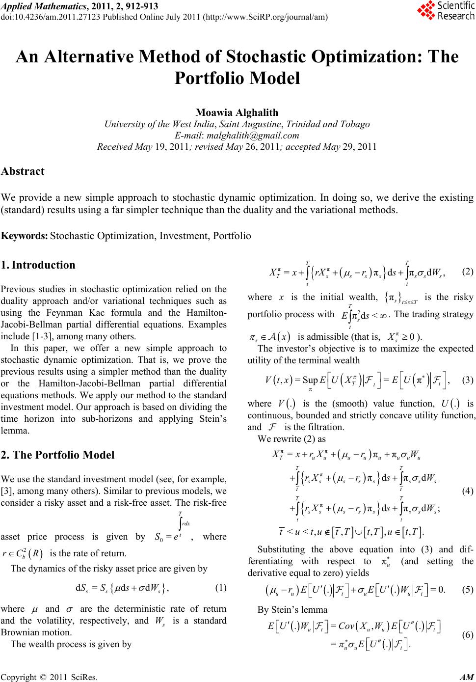Applied Mathematics, 2011, 2, 912-913

doi:10.4236/am.2011.27123 Published Online July 2011 (http://www.SciRP.org/journal/am)

An Alternative Method of Stochastic Optimization: The

Portfolio Model

Moawia Alghalith

University of the West India, Saint Augustine, Trinidad and Tobago

E-mail: [email protected]

Received May 19, 2011; revised May 26, 2011; accep te d Ma y 29, 2011

Abstract

We provide a new simple approach to stochastic dynamic optimization. In doing so, we derive the existing

(standard) results using a far simpler technique than the duality and the variational methods.

Keywords: Stochastic Optimization, Investment, Portfolio

1. Introduction

Previous studies in stochastic optimization relied on the

duality approach and/or variational techniques such as

using the Feynman Kac formula and the Hamilton-

Jacobi-Bellman partial differential equations. Examples

include [1-3], among many others.

In this paper, we offer a new simple approach to

stochastic dynamic optimization. That is, we prove the

previous results using a simpler method than the duality

or the Hamilton-Jacobi-Bellman partial differential

equations methods. We apply our method to the standard

investment model. Our approach is based on dividing the

time horizon into sub-horizons and applying Stein’s

lemma.

2. The Portfolio M odel

We use the standard investment model (see, for example,

[3], among many others). Similar to previous models, we

consider a risky asset and a risk-free asset. The risk-free

asset price process is given by where

is the rate of return.

rds







rCR

The dynamics of the risky asset price are given by



d=dd ,

ss s

SS s W



 (1)

where



and



are the deterministic rate of return

and the volatility, respectively, and

W is a standard

Brownian motion.

The wealth process is given by





ππ

=πdπd,

Tssssss

xrXr sW



 



(2)

where

is the initial wealth,



is the risky πstsT

portfolio process with . The trading strategy

πd<

Es









 is admissible (that is, ).

π0

X

The investor’s objective is to maximize the expected

utility of the terminal wealth







,=Sup= π,

Vtx EUXEU











(3)

where





.V is the (smooth) value function,





.U is

continuous, bounded and strictly concave utility function,

and is the filtration.



We rewrite (2) as













 

ππ

=ππ

πdπd

πdπd;

<<,,, ,, .

Tuuuuuuuu

ssss ss

XxrX rW

rXr sW

tututT tTutT









 

 

 



(4)

Substituting the above equation into (3) and dif-

ferentiating with respect to (and setting the

derivative equal to zero) yields

πu











uut uut

rEUEU W













=0.

(5)

By Stein’s lemma











.=, .

=..

utuut

uu t

EUWCovX WEU





























(6)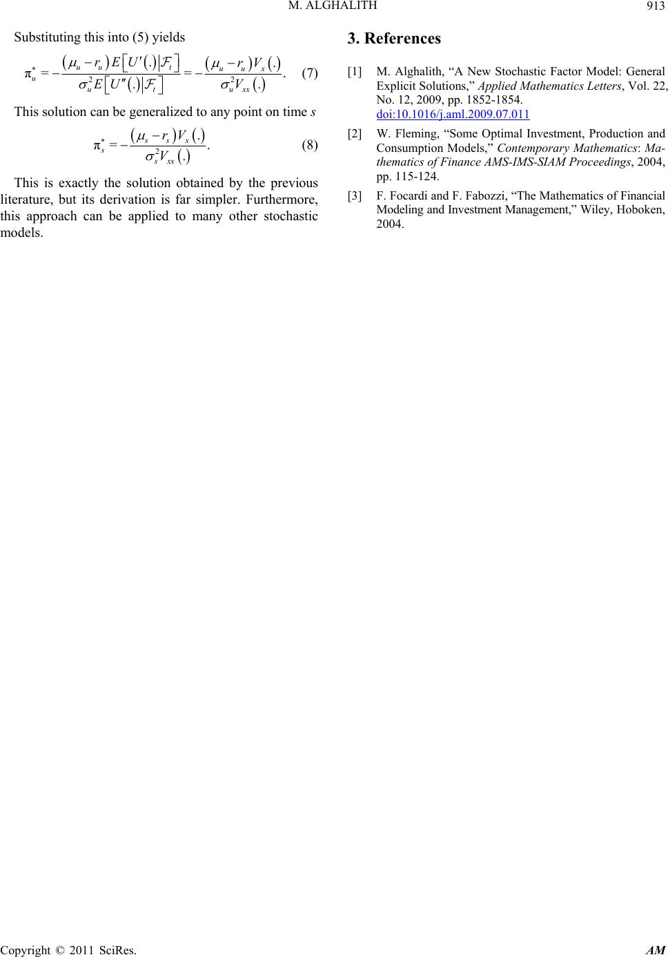

M. ALGHALITH 913

Substituting this into (5) yields



π==

uut uux

uuxx

rEU rV























.

(7)

This solution can be generalized to any point on time s



π=

ssx

ssxx







.

(8)

This is exactly the solution obtained by the previous

literature, but its derivation is far simpler. Furthermore,

this approach can be applied to many other stochastic

models.

3. References

[1] M. Alghalith, “A New Stochastic Factor Model: General

Explicit Solutions,” Applied Mathematics Letters, Vol. 22,

No. 12, 2009, pp. 1852-1854.

doi:10.1016/j.aml.2009.07.011

[2] W. Fleming, “Some Optimal Investment, Production and

Consumption Models,” Contemporary Mathematics: Ma-

thematics of Finance AMS-IMS-SIAM Proceedings, 2004,

pp. 115-124.

[3] F. Focardi and F. Fabozzi, “The Mathematics of Financial

Modeling and Investment Management,” Wiley, Hoboken,

2004.