Analytical solution of coupled non-linear second order differential equations in enzyme kinetics

doi:10.4236/ns.2011.36063

Paper Menu >>

Journal Menu >>

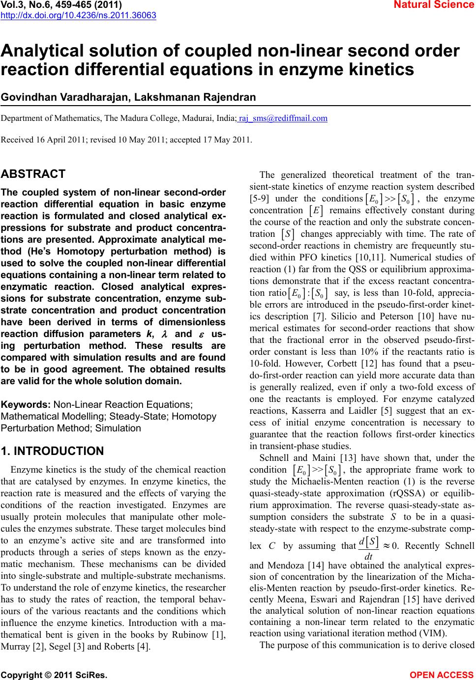Vol.3, No.6, 459-465 (2011) Natural Science

http://dx.doi.org/10.4236/ns.2011.36063

Analytical solution of coupled non-linear second order

reaction differential equations in enzyme kinetics

Govindhan Varadharajan, Lakshmanan Rajendran

Department of Mathematics, The Madura College, Madurai, India; [email protected]

Received 16 April 2011; revised 10 May 2011; accepted 17 May 2011.

ABSTRACT

The coupled system of non-linear second-order

reaction differential equation in basic enzyme

reaction is formulated and closed analytical ex-

pressions for substrate and product concentra-

tions are presented. Approximate analytical me-

thod (He’s Homotopy perturbation method) is

used to solve the coupled non-linear differential

equations containing a non-linear term related to

enzymatic reaction. Closed analytical expres-

sions for substrate concentration, enzyme sub-

strate concentration and product concentration

have been derived in terms of dimensionless

reaction diffusion parameters k,



and



us-

ing perturbation method. These results are

compared with simulation results and are found

to be in good agreement. The obtained results

are valid for the whole solution domain.

Keywords: Non-Linear Reaction Equations;

Mathematical Modelling; Steady-State; Homotopy

Perturbation Method; Simulation

1. INTRODUCTION

Enzyme kinetics is the study of the chemical reaction

that are catalysed by enzymes. In enzyme kinetics, the

reaction rate is measured and the effects of varying the

conditions of the reaction investigated. Enzymes are

usually protein molecules that manipulate other mole-

cules the enzymes substrate. These target molecules bind

to an enzyme’s active site and are transformed into

products through a series of steps known as the enzy-

matic mechanism. These mechanisms can be divided

into single-substrate and multiple-substrate mechanisms.

To understand the role of enzyme kinetics, the researcher

has to study the rates of reaction, the temporal behav-

iours of the various reactants and the conditions which

influence the enzyme kinetics. Introduction with a ma-

thematical bent is given in the books by Rubinow [1],

Murray [2], Segel [3] and Roberts [4].

The generalized theoretical treatment of the tran-

sient-state kinetics of enzyme reaction system described

[5-9] under the conditions









ES , the enzyme

concentration





E remains effectively constant during

the course of the reaction and only the substrate concen-

tration





S changes appreciably with time. The rate of

second-order reactions in chemistry are frequeuntly stu-

died within PFO kinetics [10,11]. Numerical studies of

reaction (1) far from the QSS or equilibrium approxima-

tions demonstrate that if the excess reactant concentra-

tion ratio









S say, is less than 10-fold, apprecia-

ble errors are introduced in the pseudo-first-order kinet-

ics description [7]. Silicio and Peterson [10] have nu-

merical estimates for second-order reactions that show

that the fractional error in the observed pseudo-first-

order constant is less than 10% if the reactants ratio is

10-fold. However, Corbett [12] has found that a pseu-

do-first-order reaction can yield more accurate data than

is generally realized, even if only a two-fold excess of

one the reactants is employed. For enzyme catalyzed

reactions, Kasserra and Laidler [5] suggest that an ex-

cess of initial enzyme concentration is necessary to

guarantee that the reaction follows first-order kinectics

in transient-phase studies.

Schnell and Maini [13] have shown that, under the

condition





E>>





S, the appropriate frame work to

study the Michaelis-Menten reaction (1) is the reverse

quasi-steady-state approximation (rQSSA) or equilib-

rium approximation. The reverse quasi-steady-state as-

sumption considers the substrate S to be in a quasi-

steady-state with respect to the enzyme-substrate comp-

lex C by assuming that





0. Recently Schnell

and Mendoza [14] have obtained the analytical expres-

sion of concentration by the linearization of the Micha-

elis-Menten reaction by pseudo-first-order kinetics. Re-

cently Meena, Eswari and Rajendran [15] have derived

the analytical solution of non-linear reaction equations

containing a non-linear term related to the enzymatic

reaction using variational iteration method (VIM).

The purpose of this communication is to derive closed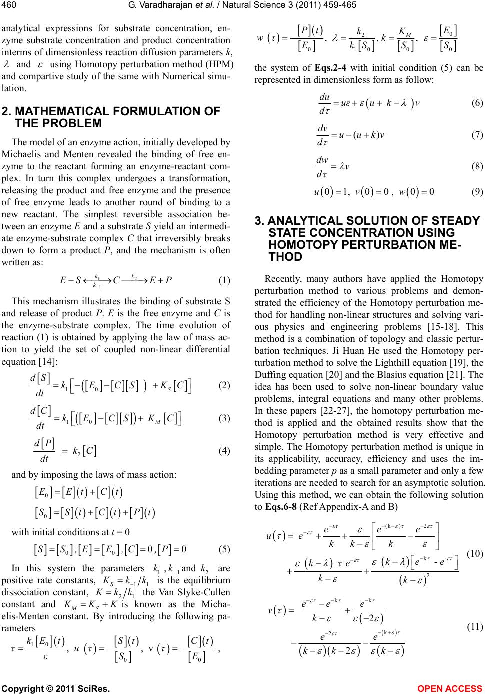

G. Varadharajan et al. / Natural Science 3 (2011) 459-465

460

analytical expressions for substrate concentration, en-

zyme substrate concentration and product concentration

interms of dimensionless reaction diffusion parameters k,



and



using Homotopy perturbation method (HPM)

and compartive study of the same with Numerical simu-

lation.

2. MATHEMATICAL FORMULATION OF

THE PROBLEM

The model of an enzyme action, initially developed by

Michaelis and Menten revealed the binding of free en-

zyme to the reactant forming an enzyme-reactant com-

plex. In turn this complex undergoes a transformation,

releasing the product and free enzyme and the presence

of free enzyme leads to another round of binding to a

new reactant. The simplest reversible association be-

tween an enzyme E and a substrate S yield an intermedi-

ate enzyme-substrate complex C that irreversibly breaks

down to form a product P, and the mechanism is often

written as:

ESC EP



 (1)

This mechanism illustrates the binding of substrate S

and release of product P. E is the free enzyme and C is

the enzyme-substrate complex. The time evolution of

reaction (1) is obtained by applying the law of mass ac-

tion to yield the set of coupled non-linear differential

equation [14]:













10 S

dS kECS KC

dt 

 



(2)













10 M

dC kE CSKC

dt 





(3)







dP kC

dt  (4)

and by imposing the laws of mass action:

















E Et Ct























S St Ct Pt

with initial conditions at t = 0

























00S S , EE , C , P (5)

In this system the parameters 1 12

,and

k k kare

positive rate constants, 11S



 is the equilibrium

dissociation constant, 21

kk the Van Slyke-Cullen

constant and MS

K Kis known as the Micha-

elis-Menten constant. By introducing the following pa-

rameters





 























, , v ,

kE tSt Ct

εSE















  







01000

, , ,

EPt kK

wτk

EkSSS





the system of Eqs.2-4 with initial condition (5) can be

represented in dimensionless form as follow:



du uεuk v





  (6)

()

dv uukv



  (7)

dw v





 (8)









01, 00 , 00uv w



 (9)

3. ANALYTICAL SOLUTION OF STEADY

STATE CONCENTRATION USING

HOMOTOPY PERTURBATION ME-

THOD

Recently, many authors have applied the Homotopy

perturbation method to various problems and demon-

strated the efficiency of the Homotopy perturbation me-

thod for handling non-linear structures and solving vari-

ous physics and engineering problems [15-18]. This

method is a combination of topology and classic pertur-

bation techniques. Ji Huan He used the Homotopy per-

turbation method to solve the Lighthill equation [19], the

Duffing equation [20] and the Blasius equation [21]. The

idea has been used to solve non-linear boundary value

problems, integral equations and many other problems.

In these papers [22-27], the homotopy perturbation me-

thod is applied and the obtained results show that the

Homotopy perturbation method is very effective and

simple. The Homotopy perturbation method is unique in

its applicability, accuracy, efficiency and uses the im-

bedding parameter p as a small parameter and only a few

iterations are needed to search for an asymptotic solution.

Using this method, we can obtain the following solution

to Eqs.6-8 (Ref Appendix-A and B)



 



(k )2

eee

uekk k

kee

 























 















(10)

 

 



ee e

kk k

 











 

 













(11)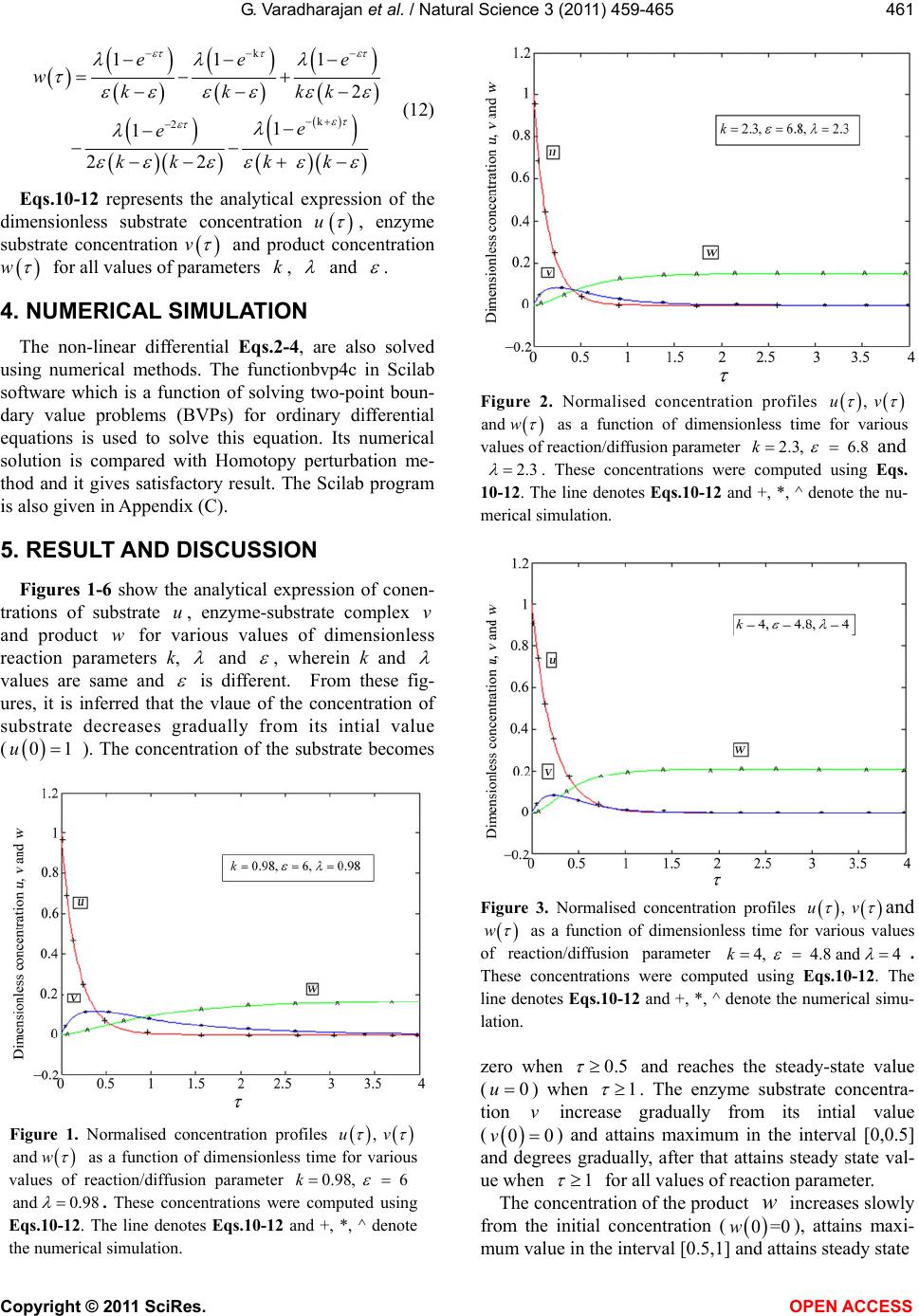

G. Varadharajan et al. / Natural Science 3 (2011) 459-465

461



 





11 1

ee e

wkkkk

kkk k







 













 





 









 

(12)

Eqs.10-12 represents the analytical expression of the

dimensionless substrate concentration u







, enzyme

substrate concentration v







and product concentration







for all values of parameters k,



and



4. NUMERICAL SIMULATION

The non-linear differential Eqs.2-4, are also solved

using numerical methods. The functionbvp4c in Scilab

software which is a function of solving two-point boun-

dary value problems (BVPs) for ordinary differential

equations is used to solve this equation. Its numerical

solution is compared with Homotopy perturbation me-

thod and it gives satisfactory result. The Scilab program

is also given in Appendix (C).

5. RESULT AND DISCUSSION

Figures 1-6 show the analytical expression of conen-

trations of substrate u, enzyme-substrate complex v

and product w for various values of dimensionless

reaction parameters k,



and



, wherein k and



values are same and



is different. From these fig-

ures, it is inferred that the vlaue of the concentration of

substrate decreases gradually from its intial value

(



01 u). The concentration of the substrate becomes

Figure 1. Normalised concentration profiles







, uv







and w



as a function of dimensionless time for various

values of reaction/diffusion parameter 0.98, 6 k





and 0.98



. These concentrations were computed using

Eqs.10-12. The line denotes Eqs.10-12 and +, *, ^ denote

the numerical simulation.

Figure 2. Normalised concentration profiles









, uv







and w



as a function of dimensionless time for various

values of reaction/diffusion parameter 2.3, 6.8 k



and

2.3





. These concentrations were computed using Eqs.

10-12. The line denotes Eqs.10-12 and +, *, ^ denote the nu-

merical simulation.

Figure 3. Normalised concentration profiles









, uv



and







as a function of dimensionless time for various values

of reaction/diffusion parameter 4, 4.8 and 4k





 

These concentrations were computed using Eqs.10-12. The

line denotes Eqs.10-12 and +, *, ^ denote the numerical simu-

lation.

zero when 0.5



 and reaches the steady-state value

(0u



) when 1



. The enzyme substrate concentra-

tion v increase gradually from its intial value

(





00v



) and attains maximum in the interval [0,0.5]

and degrees gradually, after that attains steady state val-

ue when 1



 for all values of reaction parameter.

The concentration of the product w increases slowly

from the initial concentration (



0=0w), attains maxi-

mum value in the interval [0.5,1] and attains steady state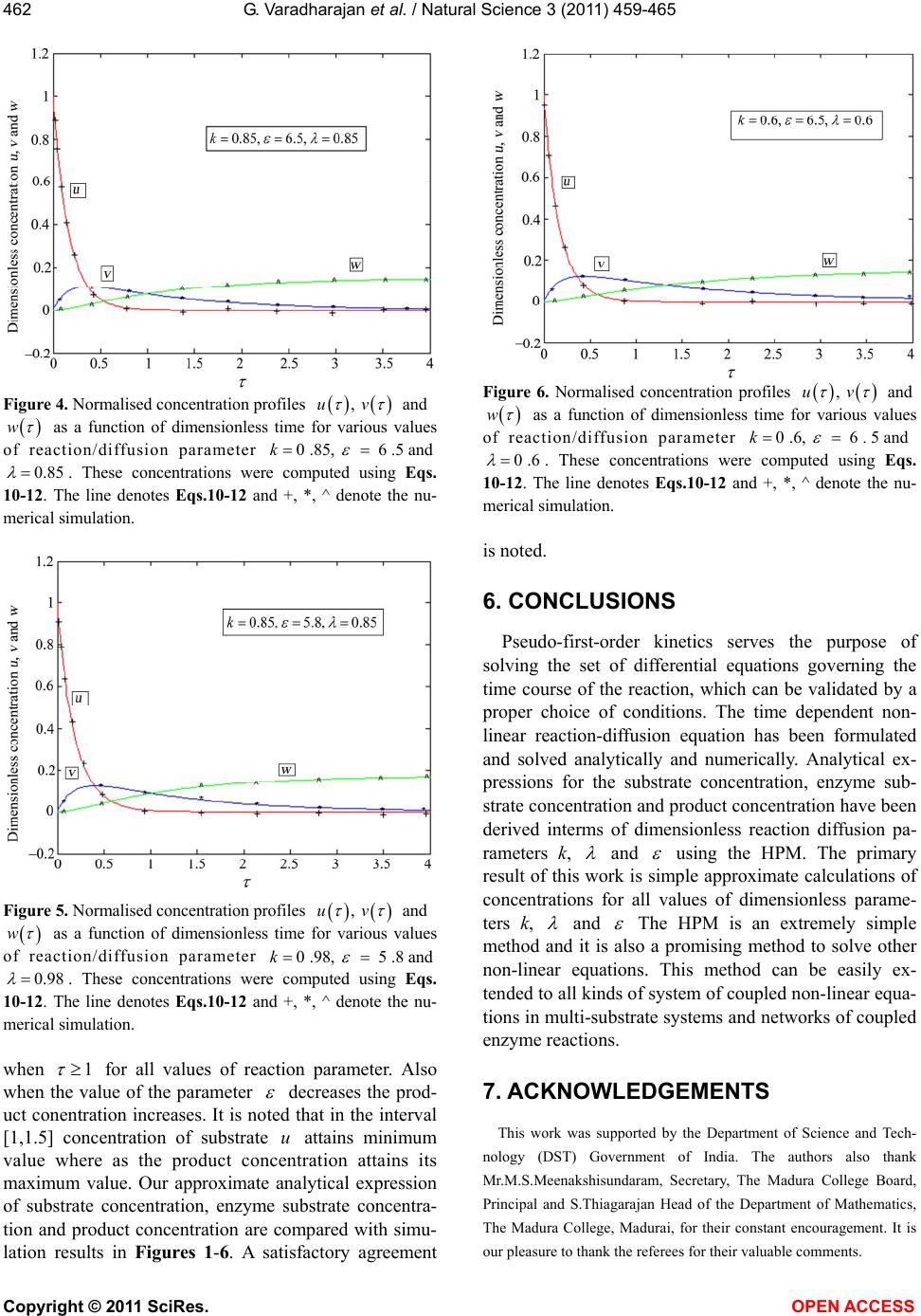

G. Varadharajan et al. / Natural Science 3 (2011) 459-465

462

Figure 4. Normalised concentration profiles







, anduv







as a function of dimensionless time for various values

of reaction/diffusion parameter 0 .85, 6 .5 andk





0.85



. These concentrations were computed using Eqs.

10-12. The line denotes Eqs.10-12 and +, *, ^ denote the nu-

merical simulation.

Figure 5. Normalised concentration profiles







, anduv







as a function of dimensionless time for various values

of reaction/diffusion parameter 0 .98, 5 .8 andk





0.98



. These concentrations were computed using Eqs.

10-12. The line denotes Eqs.10-12 and +, *, ^ denote the nu-

merical simulation.

when 1



 for all values of reaction parameter. Also

when the value of the parameter



decreases the prod-

uct conentration increases. It is noted that in the interval

[1,1.5] concentration of substrate u attains minimum

value where as the product concentration attains its

maximum value. Our approximate analytical expression

of substrate concentration, enzyme substrate concentra-

tion and product concentration are compared with simu-

lation results in Figures 1-6. A satisfactory agreement

Figure 6. Normalised concentration profiles







, anduv









as a function of dimensionless time for various values

of reaction/diffusion parameter 0 .6, 6 5 and k.





0 .6





. These concentrations were computed using Eqs.

10-12. The line denotes Eqs.10-12 and +, *, ^ denote the nu-

merical simulation.

is noted.

6. CONCLUSIONS

Pseudo-first-order kinetics serves the purpose of

solving the set of differential equations governing the

time course of the reaction, which can be validated by a

proper choice of conditions. The time dependent non-

linear reaction-diffusion equation has been formulated

and solved analytically and numerically. Analytical ex-

pressions for the substrate concentration, enzyme sub-

strate concentration and product concentration have been

derived interms of dimensionless reaction diffusion pa-

rameters k,



and



using the HPM. The primary

result of this work is simple approximate calculations of

concentrations for all values of dimensionless parame-

ters k,



and



The HPM is an extremely simple

method and it is also a promising method to solve other

non-linear equations. This method can be easily ex-

tended to all kinds of system of coupled non-linear equa-

tions in multi-substrate systems and networks of coupled

enzyme reactions.

7. ACKNOWLEDGEMENTS

This work was supported by the Department of Science and Tech-

nology (DST) Government of India. The authors also thank

Mr.M.S.Meenakshisundaram, Secretary, The Madura College Board,

Principal and S.Thiagarajan Head of the Department of Mathematics,

The Madura College, Madurai, for their constant encouragement. It is

our pleasure to thank the referees for their valuable comments.

G. Varadharajan et al. / Natural Science 3 (2011) 459-465

463

REFERENCES

[1] Rubinow, S.I. (1975) Introduction to Mathematical Biol-

ogy. Wiley, New York.

[2] Murray, J.D. (1989) Mathematical biology. Springer

Verlag, Berlin.

[3] Segel, L.A. (1980) Mathematical models in molecular

and cellular biology. Cambridge University Press, Cam-

bridge.

[4] Roberts, D.V. (1977) Enzyme kinetics. Cambridge Uni-

versity Press, Cambridge.

[5] Kasserra, H.P. and Laidler, K.J. (1970) Transient-phase

studies of a trypsin-catalyzed reaction. Canadian Journal

of Chemistry, 48, 1793-1802. doi:10.1139/v70-298

[6] Pettersson, G. (1976) The transient-state kinetics of

two-substrate enzyme systems operating by an ordered

ternary-complex mechanism. European Journal of Bio-

chemistry, 69, 273-278.

d oi:10.1111/j.14 32-1033.1976.tb10883.x

[7] Pettersson, G. (1978) A generalized theoretical treatment

of the transient-state kinetics of enzymic reaction sys-

tems far from equilibrium. Acta Chemica Scandinavica -

Series B, 32, 437-446.

doi:10.3891/acta.chem.scand.32b-0437

[8] Gutfreund, H. (1995) Kinetics for life sciences: Recep-

tors, transmitters and catalysis. Cambridge University

Press, Cambridge. doi:10.1017/CBO9780511626203

[9] Fersht, A.R. (1999) Structure and mechanism in protein

science: A guide to enzyme catalysis and protein folding.

Freeman, New York.

[10] Silicio, F. and Peterson, M.D. (1961) Ratio errors in

pseudo first order reactions. Journal of Chemical Educa-

tion, 38, 576-577. doi:10.1021/ed038p576

[11] Moore, J.W. and Pearson, R.G. (1981) Kinetics and Me-

chanism. Wiley, New York.

[12] Corbett, J.F. (1972) Pseudo first-order kinetics. Journal

of Chemical Education, 49, 663. doi:10.1021/ed049p663

[13] Schnell, S. and Maini, P.K. (2000) Enzyme kinetics at

high enzyme concentration. Bulletin of Mathematical Bi-

ology, 62, 483-499. doi:10.1006/bulm.1999.0163

[14] Schnell, S. and Mendoza, C. (2004) The condition for

pseudo-first-order kinetics in enzymatic reaction is inde-

pendent of the initial enzyme concentration. Journal of

Biophysical Chemistry, 107, 165-174.

doi:10.1016/j.bpc.2003.09.003

[15] Meena, A., Eswari, A. and Rajendran, L. (2010) Mathe-

matical modelling of enzyme kinetics reaction mecha-

nism and analytical sloutions of non-linear reaction equa-

tions. Journal of Mathematical Chemistry, 48, 179-186.

doi:10.1007/s10910-009-9659-5

[16] Li, S.J. and Liu, Y.X. (2006) An improved approach to

nonlinear dynamical system identification using pid neu-

ral networks. International Journal of Nonlinear Science

and Numerical Simulation, 7, 177-182.

[17] Mousa, M.M., Ragab, S.F. and Nturforsch, Z. (2008)

Application of the homotopy perturbation method to lin-

ear and nonlinear schrödinger equations. Zeitschrift für

Naturforschung, 63, 140-144.

[18] He, J.H. (1999) Homotopy perturbation technique.

Computer Methods in Applied Mechanics and Engineer-

ing, 178, 257-262.

[19] He, J.H. (2003) Homotopy perturbation method: a new

nonlinear analytical Technique. Applied Mathematics and

Computation, 135, 73-79.

doi:10.1016/S0096-3003(01)00312-5

[20] He, J.H. (2003) A Simple perturbation approach to Bla-

sius equation. Applied Mathematics and Computation,

140, 217-222. doi:10.1016/S0096-3003(02)00189-3

[21] He, J.H. (2006) Some asymptotic methods for strongly

nonlinear equations. International Journal of Modern

Physics B, 20, 1141-1199.

doi:10.1142/S0217979206033796

[22] He, J.H., Wu, C.G. and Austin, F. (2010) The variational

iteration method which should be followed. Nonlinear

Science Letters A, 1, 1-30.

[23] He, J.H. (2003) A coupling method of a homotopy tech-

nique and a perturbation technique for non-linear prob-

lems. International Journal of Non-Linear Mechanics, 35,

37-43. doi:10.1016/S0020-7462(98)00085-7

[24] Ganji, D.D., Amini, M. and Kolahdooz, A. (2008) Ana-

lytical investigation of hyperbolic equations via he’s me-

thods. American Journal of Engineering and Applied

Sciences, 1, 399-407.

[25] Loghambal, S. and Rajendran, L. (2010) Mathematical

modeling of diffusion and kinetics of amperometric im-

mobilized enzyme electrodes. Electrochimica Acta, 55,

5230-5238. doi:10.1016/j.electacta.2010.04.050

[26] Meena, A. and Rajendran, L. (2010) Mathematical mod-

eling of amperometric and potentiometric biosensors and

system of non-linear equations—Homotopy perturbation

approach. Journal of Electroanalytical Chemistry, 644,

50-59. doi:10.1016/j.jelechem.2010.03.027

[27] Eswari, A. and Rajendran, L. (2010) Analytical solution

of steady state current an enzyme modified microcylinder

electrodes. Journal of Electroanalytical Chemistry, 648,

36-46. doi:10.1016/j.jelechem.2010.07.002

G. Varadharajan et al. / Natural Science 3 (2011) 459-465

464

APPENDIX A

Basic idea of Homotopy – perturbation me-

thod (HPM)

To explain this method, let us consider the following

function

 

0, Awf rr (A1)

With the boundary conditions of

,0,

Bw r











 (A2)

where

, B,





r and  are a general differential

operator , a boundary operator, a known analytical func-

tion and the boundary of the domain , respectively.

Generally speaking, the operator

can be divided into

a linear part L and a nonlinear partN. Eq.A1 can

therefore, be written as

 





0LwNwfr (A3)

By the Homotopy technique, we construct a Homo-

topy







,: 0,1zrp R which satisfies

 





 



0 [0,1],

Hzpp LzLw

pAzf rpr



 





(A4)























,0HzpLzLw pLwpNzfr 



(A5)

where





0,1p is an embedding parameter, while 0

is an initial approximation of Eq.A1, which satisfies the

boundary conditions. Obviously, from Eqs.A4 and A5,

we will have

 



,00 HzLzLw  (A6)



,1 0.HzAz fr (A7)

The changing process of p from zero to unity is just

that of



,zrp from 0

w to



.wr In topology, this is

called deformation, while



Lz Lw and

 

zfr are called Homotopy. According to the

HPM, we can first use the embedding parameter p as a

“small parameter”, and assume that the solutions of Eqs.

A4 and A5 can be written as a power series in p:

01 2

.....zzpzpz (A8)

Setting 1p results in the approximate solution of Eq.

012

lim .....

wzzzz





(A9)

The combination of the perturbation method and the

Homotopy method is called the HPM, which eliminates

the drawbacks of the traditional perturbation methods

while keeping all its advantages.

APPENDIX B

Solution of the Eqs.2 and 3 using Homotopy perturba-

tion method. In this Appendix, we indicate how Eqs.10,

11 and 12 in this paper are derived. Furthermore, a

Homotopy was constructed to determine the solution of

Eqs.2 and 3.



puuvk vv





 















 





(B1)



1- 0

dv dv

pkvpkvuuv











(B2)

and the initial approximations are as follows:





(0)1, 00uv



 (B3)

approximate solutions of (B1) and (B2) are

0123

..................uupupu pu  (B4)

and

0123

..................vv pvpvpv  (B5)

Substituting Eqs.B4 and B5 into Eqs.B1 and B2 and

comparing the coefficients of like powers of p

: 0







 (B6)

1000 0

: 0

puuvkvv









(B7)

201101 1

: =0

puuvuvkvv

 



  (B8)

And 00

: 0

pkv





 (B9)

10 00

: 0

pkvuuv





 

(B10)

210110

: + =0

pkvuuvuv



 (B11)

Solving the Eqs .B 6-B11, and using the boundary con-

ditions (B3), we can find the following results





0 ue







 (B12)





1= 0u



(B13)



(k )2

eee

ukk k

 











 











G. Varadharajan et al. / Natural Science 3 (2011) 459-465

465

 



kee



























 (B14)

And



00v



 (B15)



 







 (B16)

 

 



222

eee

vkkk k

















 

 

(B17)

According to the HPM, we can conclude that

 

012

lim

uuuuu





 (B18)

 

012

lim

vvvvv





 (B19)

Using Eqs. B12 , B13 and B14 in Eqs.B18 and Eqs.

B15, B16 and B17 in Eqs.B19, we obtain the final re-

sults as described in Eqs.10 and 11. The dimensionless

concentration of the product is given by

 









11 1

kkkk2

2kk2k k

ee e



 





 



 







 







 









 



(B20)

The above equation represent the new analytical ex-

pression of product





for all values of parameters

, and k





which is given in Eq.12.

APPENDIX C

Scilab program to find the solutions of the Eqs. 6-9

function main123456

options= odeset('RelTol',1e-6,'Stats','on');

%initial conditions

x0 = [1; 0;0];

tspan = [0 10];

tic

[t,x] = ode45(@TestFunction,tspan,x0,options);

toc

figure

hold on

plot(t, x(:,1))

plot(t, x(:,2))

plot(t, x(:,3))

legend('x1','x2')

ylabel('x')

xlabel('t')

return

function [dx_dt]= TestFunction(t,x)

b=6.5;a=0.85;d=0.85;

dx_dt(1)=-b*x(1)+b*(x(1)+a-d)*x(2);

dx_dt(2) =x(1)-((x(1)+a)*x(2));

dx_dt(3) =d*x(2);

dx_dt = dx_dt';

return

APPENDIX D

Nomenclature

Symboles





E Enzyme concentration (







C Enzyme-substrate complex (







S Substrate concentation(







E Initial enzyme concentration (







S Initial substrate concentraton (



Michaelis-Menten constant

Equilibrium dissociation constant

(



K Van Slyke-Cullen constant (



112

k k k Positive rate constants (None)

, , k





Reaction diffusion parameter (None)

u Dimensionless Substrate concentra-

tion (None)

v Dimensionless enzyme substrate con-

centration (None)

w Dimensionless product concentration

(None)

t Time (Sec)



Dimensionless time (None)