Fitting of precipitation in 49 European capitals from 1901 to 1998 using random walk

doi:10.4236/ns.2011.36059

Paper Menu >>

Journal Menu >>

Vol.3, No.6, 430-435 (2011) Natural Science

http://dx.doi.org/10.4236/ns.2011.36059

Fitting of precipitation in 49 European capitals from 1901

to 1998 using random walk

Shaomin Yan1, Guang Wu1,2*

1State Key Laboratory of Non-Food Biomass Enzyme Technology, National Engineering Research Center for Non-Food Biorefinery,

Guangxi Key Laboratory of Biorefinery, Guangxi Academy of Sciences, Nanning, China

2DreamSciTech Consulting, Shenzhen, Guangdong, China; *corresponding author: [email protected]

Received 15 March 2011; revised 5 April 2011; accepted 15 April 2011.

ABSTRACT

Mathematical modeling of precipitation is an

important step to understand the precipitation

patterns, and paves the way to possibly predict

the precipitation. In this study, we attempt to

use the random walk model to fit the annual

precipitation in 49 European capitals from 1901

to 1998. At first, we used the simplest random

walk model to fit the precipitation walk, which is

the conversion of recorded precipitations into

±1 format, and then we used a more complex

random walk model to fit the recorded precipi-

tations. The results show that the random walk

models can fit both precipitation walk and re-

corded precipitation. Thus this study provides a

model to describe the precipitation patterns

during this period in these cities.

Keywords: European Capital; Fitting; Precipitation;

Random Walk

1. INTRODUCTION

Mathematical description of precipitation is important,

not only because it can help up better understand the

precipitation pattern, but also it can provide a tool to

possibly predict the precipitation. However, a mathe-

matical model is not so easy to build because the pre-

cipitation is related to enormous factors, which lead to

the difficulty to use a deterministic model to describe the

precipitation. Technologically, the deterministic model is

generally based on the cause-consequence relationship,

which can be modeled as differential equations. As many

cause-consequence relationships coexist in precipitation

process, one would have great difficulty to separate var-

ious cause-consequence relationships notably because

we cannot conduct a control experiment to determine

each cause-consequence relationship. Still we have many

unknown factors, which are not possible to include in a

deterministic model. Computationally, a deterministic

model with many factors would have great difficulty to

fit the recorded data.

In this context, we may consider alternative models,

such as stochastic models, of which the random walk is

an important model to describe natural phenomena, for

examples, stock pattern [1] and temperature change [2,

3]. Thus an interesting question raised here is whether

the random walk model can describe the precipitation

along with other powerful deterministic models? Practi-

cally, we cannot find any clearly visible patterns in year-

to-year precipitations if we scrutinize the recorded pre-

cipitations over year in certain geographic location. The

non-patterned precipitations would provide us with the

opportunity to use the random walk model to fit.

To answer this question, we use the random walk

model to fit the annual precipitations in 49 European

capitals from 1901 to m 1998 in this study.

2. MATERIALS AND METHODS

2.1. Data

The precipitations recorded in these 49 European cap-

itals from 1901 to 1998 were obtained from the website

of Oak Ridge National Laboratory [4], and their latitudes

and longitudes were determined using Get Lat Lon [5] in

order to define the precise precipitations according to the

0.5˚ by 0.5˚ latitude and longitude grid-box.

2.2. Precipitation Walk

We use the simplest random walk model, which starts

at zero and moves by ±1 with equal probability at each

step [6]. As the precipitation is in decimal format, thus

we convert the precipitation into ±1 format as precipita-

tion walk. Technically, when the precipitation at certain

year is higher than its previous year, we classify it as 1,

otherwise we classify it as –1, and then we add them

together as the random walk does.

S. M. Yan et al. / Natural Science 3 (2011) 430-435

431

2.3. Generating Random Walk

We use the SigmaPlot [7] with different seeds to gen-

erate random sequences ranged from –1 to 1, and then

we classify a random number as 1 if it is larger than its

previous one and as –1 if it is smaller than its previous

one. Thereafter we add the classified ±1 as random walk.

2.4. Searching for Seed

To the best of our knowledge, there is no algorithm

available to find the right seed, which produces the best

fit between random walk and observed data. However,

this is not a problem with current computational tech-

nique, because we can simply search all the seeds in

searching space and compare their outcomes.

2.5. Fitting Recorded Precipitation

Hereafter, we use a more complicated random walk

model [8] to fit the recorded precipitation, which is in

decimal format. In plain words, the simplest random

walk comes from tossing of double-sided coin, while

this random walk could be regarded as tossing of dice,

which can be not only six-sided but as many as the de-

cimal data. In this way, we generate random numbers,

and add them to construct the random walk, and the fit-

ting is again to search the best seed that generates best

fit.

2.6. Comparison

For determining the best seed, we compare the least

squared errors between precipitation walk and random

walk, and between recorded precipitation and random

precipitation generated from different seeds.

3. RESULTS AND DISCUSSION

Table 1 shows how we construct a precipitation walk

and its corresponding random walk. For the precipitation

walk, we have the follows: 1) the starting point is the

annual precipitation in 1901, 847 mm (cell 2, column 2),

and this starting point corresponds zero in sense of pre-

cipitation walk (cell 2, column 4); 2) the annual precipi-

tation in 1902 is 737 mm (cell 3, column 2), which is

smaller than the first one, 847 mm (cell 2, column 2), so

we assign –1 as precipitation step (cell 3, column 3), 3)

the precipitation walk is –1 (0 + (–1)) (cell 3, column 4),

and 4) the similar computation is applied to all the data

in columns 2, 3, and 4.

For the random walk, we have the follows: 1) a good

seed we found is 6.98078, and this seed generates a se-

ries of random numbers (column 5), 2) the first random

number, 0.36795 (cell 2, column 5), is considered as the

starting point corresponding to 0 in random walk (cell 2,

column 7), 3) the second random number, –0.74132 (cell

3, column 5), is smaller than the first random number,

0.36795 (cell 2, column 5), so we assign –1 (cell 3,

column 6), 4) the random walk is –1 (0 + (–1)) (cell 3,

column 7), and 5) the similar procedure is applied to all

the data in columns 5, 6, and 7. In the same manner, we

construct the precipitation walk and random walk.

The figures in the left side of Figure 1 show the fit-

tings of precipitation walk in 7 European capitals using

random walk model. As can be seen, the curve generated

by random walk generally passes through the precipita-

tion walk. Theoretically, the chance for a completely

perfect fitting of precipitation walk is an extremely rare

event. In our case, there are 98 annual precipitations,

thus the completely perfect fitting has the chance of

(1/2)98 theoretically, which is extremely small. Clearly

this probability is very difficult to achieve in limited

time because the space of our search is limited to one

million of seed. So the fitting results in the left side of

Figure 1 suggest that a good seed can be relatively eas-

ily found, thus we consider that the random walk can

describe the precipitation walk, although we cannot

compare our results with other results because the other

models do not set an equal-sized step.

Actually we can view the precipitation walk, which is

the conversion from its annual precipitation, as the trend

of recorded precipitation. This is so because this trend

answers the very basic question of whether the precipita-

tion at certain year is larger (1) or smaller (–1) than its

previous year.

Yet, the cities in Figure 1 cross the whole Europe,

thus there would be uncountable factors affecting the

precipitations, but the random walk still can fit them.

This furthermore suggests that the random walk can de-

scribe the precipitation patterns in terms of precipitation

walk.

Table 2 shows how we use a random walk model to

fit the recorded annual precipitation, here we only need

to construct the random precipitation: 1) the starting

point is the first recorded annual precipitation, which is

847 mm (cell 2 in column 2 and column 4), 2) the seed

for Table 2 is 1.31923, 3) the first random number gen-

erated by the seed is 64.17878 (cell 3, column 3), 4) we

add this value to the previous precipitation datum (847)

resulting in 911.17878 mm (cell 3, column 4), and 5)

along this procedure, we get the random precipitation in

column 4.

The figures in the right side of Figure 1 display the

fittings of recorded precipitation with random precipita-

tion in 7 European capitals. In these figures, the precipi-

tation demonstrates very remarkable fluctuations along

the time course, which do not show any clear sign of

visible pattern. This is the basis for conducting random-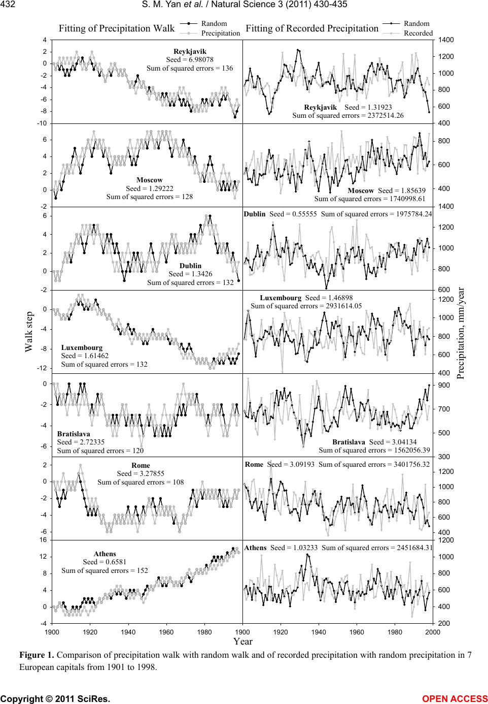

S. M. Yan et al. / Natural Science 3 (2011) 430-435

432

Fitting of Precipitation Walk

-10

-8

-6

-4

-2

Random

Precipitation

Reykjavik

Seed = 6.98078

Sum of squared errors = 136

Fitting of Recorded Precipitation

400

600

800

1000

1200

1400

Random

Recorded

-2

Moscow

Seed = 1.29222

Sum of squared errors = 128

-2

Walk step

-12

-8

-4

1900 1920 1940 1960 1980

-4

Dublin

Seed = 1.3426

Sum of squared errors = 132

Luxembourg

Seed = 1.61462

Sum of squared errors = 132

At hens

Seed = 0.6581

Sum of squared errors = 152

-6

-4

-2

-6

-4

-2

Bratislava

Seed = 2.72335

Sum of squared errors = 120

Rome

Seed = 3.27855

Sum of squared errors = 108

Reykjavik Seed = 1.31923

Sum of squared errors = 2372514.26

400

600

800

Moscow Seed = 1.85639

Sum of squared errors = 1740998.61

600

800

1000

1200

1400

Dublin Seed = 0.55555 Sum of squared errors = 1975784.24

Precipitation, mm/year

400

600

800

1000

1200

Luxembourg Seed = 1.46898

Sum of squared errors = 2931614.05

300

500

700

900

Bratislava Seed = 3.04134

Sum of squared errors = 1562056.39

400

600

800

1000

1200

Rome Seed = 3.09193 Sum of squared errors = 3401756.32

Year

1900 1920 1940 1960 1980 2000

200

400

600

800

1000

1200

Athens Seed = 1.03233 Sum of squared errors = 2451684.31

Figure 1. Comparison of precipitation walk with random walk and of recorded precipitation with random precipitation in 7

European capitals from 1901 to 1998.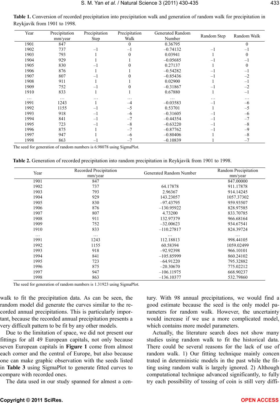

S. M. Yan et al. / Natural Science 3 (2011) 430-435

433

Table 1. Conversion of recorded precipitation into precipitation walk and generation of random walk for precipitation in

Reykjavík from 1901 to 1998.

Year Precipitation

mm/year

Precipitation

Step

Precipitation

Walk

Generated Random

Number Random Step Random Walk

1901 847 0 0.36795 0

1902 737 –1 –1 –0.74132 –1 –1

1903 793 1 0 0.03941 1 0

1904 929 1 1 –0.05685 –1 –1

1905 830 –1 0 0.27137 1 0

1906 876 1 1 –0.54282 –1 –1

1907 807 –1 0 –0.85436 –1 –2

1908 911 1 1 0.02900 1 –1

1909 752 –1 0 –0.31867 –1 –2

1910 833 1 1 0.67880 1 –1

… … … … … … …

1991 1243 1 –4 –0.03583 –1 –6

1992 1155 –1 –5 0.53701 1 –5

1993 918 –1 –6 –0.31605 –1 –6

1994 841 –1 –7 –0.44354 –1 –7

1995 723 –1 –8 –0.63220 –1 –8

1996 875 1 –7 –0.87762 –1 –9

1997 947 1 –6 –0.80406 1 –8

1998 863 –1 –7 –0.10839 1 –7

The seed for generation of random numbers is 6.98078 using SigmaPlot.

Table 2. Generation of recorded precipitation into random precipitation in Reykjavík from 1901 to 1998.

Year Recorded Precipitation

mm/year Generated Random Number Random Precipitation

mm/year

1901 847 847.00000

1902 737 64.17878 911.17878

1903 793 2.96367 914.14245

1904 929 143.23057 1057.37302

1905 830 –97.43795 959.93507

1906 876 –130.95922 828.97585

1907 807 4.73200 833.70785

1908 911 132.97379 966.68164

1909 752 –32.00623 934.67541

1910 833 –110.27817 824.39724

… … … …

1991 1243 112.18813 998.44105

1992 1155 60.58394 1059.02499

1993 918 –92.92398 966.10101

1994 841 –105.85999 860.24102

1995 723 –64.91220 795.32882

1996 875 –20.30670 775.02212

1997 947 –106.11975 668.90237

1998 863 –136.10377 532.79860

The seed for generation of random numbers is 1.31923 using SigmaPlot.

walk to fit the precipitation data. As can be seen, the

random model did generate the curves similar to the re-

corded annual precipitations. This is particularly impor-

tant, because the recorded annual precipitation presents a

very difficult pattern to be fit by any other models.

Due to the limitation of space, we did not present our

fittings for all 49 European capitals, not only because

seven European capitals in Figure 1 come from almost

each corner and the central of Europe, but also because

one can make graphic observation with the seeds listed

in Table 3 using SigmaPlot to generate fitted curves to

compare with recorded ones.

The data used in our study spanned for almost a cen-

tury. With 98 annual precipitations, we would find a

good estimate because the seed is the only model pa-

rameters for random walk. However, the uncertainty

would increase if we use a more complicated model,

which contains more model parameters.

Actually, the literature search does not show many

studies using random walk to fit the historical data.

There could be several reasons for the lack of use of

random walk. 1) Our fitting technique mainly concen

trated in deterministic models in the past while the fit-

ting using random walk is largely ignored. 2) Although

computational technique advanced significantly, to fully

try each possibility of tossing of coin is still very diffi-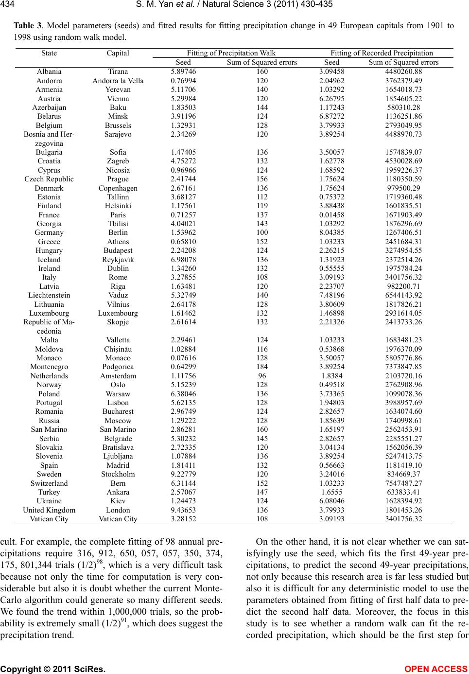

S. M. Yan et al. / Natural Science 3 (2011) 430-435

434

Table 3. Model parameters (seeds) and fitted results for fitting precipitation change in 49 European capitals from 1901 to

1998 using random walk model.

State Fitting of Precipitation Walk Fitting of Recorded Precipitation

Capital

Seed Sum of Squared errors Seed Sum of Squared errors

Albania Tirana 5.89746 160 3.09458 4480260.88

Andorra Andorra la Vella 0.76994 120 2.04962 3762379.49

Armenia Yerevan 5.11706 140 1.03292 1654018.73

Austria Vienna 5.29984 120 6.26795 1854605.22

Azerbaijan Baku 1.83503 144 1.17243 580310.28

Belarus Minsk 3.91196 124 6.87272 1136251.86

Belgium Brussels 1.32931 128 3.79933 2793049.95

Bosnia and Her-

zegovina

Sarajevo 2.34269 120 3.89254 4488970.73

Bulgaria Sofia 1.47405 136 3.50057 1574839.07

Croatia Zagreb 4.75272 132 1.62778 4530028.69

Cyprus Nicosia 0.96966 124 1.68592 1959226.37

Czech Republic Prague 2.41744 156 1.75624 1180350.59

Denmark Copenhagen 2.67161 136 1.75624 979500.29

Estonia Tallinn 3.68127 112 0.75372 1719360.48

Finland Helsinki 1.17561 119 3.88438 1601835.51

France Paris 0.71257 137 0.01458 1671903.49

Georgia Tbilisi 4.04021 143 1.03292 1876296.69

Germany Berlin 1.53962 100 8.04385 1267406.51

Greece Athens 0.65810 152 1.03233 2451684.31

Hungary Budapest 2.24208 124 2.26215 3274954.55

Iceland Reykjavík 6.98078 136 1.31923 2372514.26

Ireland Dublin 1.34260 132 0.55555 1975784.24

Italy Rome 3.27855 108 3.09193 3401756.32

Latvia Riga 1.63481 120 2.23707 982200.71

Liechtenstein Vaduz 5.32749 140 7.48196 6544143.92

Lithuania Vilnius 2.64178 128 3.80609 1817826.21

Luxembourg Luxembourg 1.61462 132 1.46898 2931614.05

Republic of Ma-

cedonia

Skopje 2.61614 132 2.21326 2413733.26

Malta Valletta 2.29461 124 1.03233 1683481.23

Moldova Chişinău 1.02884 116 0.53868 1976370.09

Monaco Monaco 0.07616 128 3.50057 5805776.86

Montenegro Podgorica 0.64299 184 3.89254 7373847.85

Netherlands Amsterdam 1.11756 96 1.8384 2103720.16

Norway Oslo 5.15239 128 0.49518 2762908.96

Poland Warsaw 6.38046 136 3.73365 1099078.36

Portugal Lisbon 5.62135 128 1.94803 3988957.69

Romania Bucharest 2.96749 124 2.82657 1634074.60

Russia Moscow 1.29222 128 1.85639 1740998.61

San Marino San Marino 2.86281 160 1.65197 2562453.91

Serbia Belgrade 5.30232 145 2.82657 2285551.27

Slovakia Bratislava 2.72335 120 3.04134 1562056.39

Slovenia Ljubljana 1.07884 136 3.89254 5247413.75

Spain Madrid 1.81411 132 0.56663 1181419.10

Sweden Stockholm 9.22779 120 3.24016 834669.37

Switzerland Bern 6.31144 152 1.03233 7547487.27

Turkey Ankara 2.57067 147 1.6555 633833.41

Ukraine Kiev 1.24473 124 6.08046 1628394.92

United Kingdom London 9.43653 136 3.79933 1801453.26

Vatican City Vatican City 3.28152 108 3.09193 3401756.32

cult. For example, the complete fitting of 98 annual pre-

cipitations require 316, 912, 650, 057, 057, 350, 374,

175, 801,344 trials (1/2)98, which is a very difficult task

because not only the time for computation is very con-

siderable but also it is doubt whether the current Monte-

Carlo algorithm could generate so many different seeds.

We found the trend within 1,000,000 trials, so the prob-

ability is extremely small (1/2)91, which does suggest the

precipitation trend.

On the other hand, it is not clear whether we can sat-

isfyingly use the seed, which fits the first 49-year pre-

cipitations, to predict the second 49-year precipitations,

not only because this research area is far less studied but

also it is difficult for any deterministic model to use the

parameters obtained from fitting of first half data to pre-

dict the second half data. Moreover, the focus in this

study is to see whether a random walk can fit the re-

corded precipitation, which should be the first step for

S. M. Yan et al. / Natural Science 3 (2011) 430-435

435

the predictions that need many studies in the future.

Currently, no results are available from other models

on fitting the precipitation of these cities for comparison.

However, our results are encouraging because the ran-

dom walk model provides a way to describe the precipi-

tation pattern.

In conclusion, the results show that the random walk

model can describe the annual precipitation pattern.

4. ACKNOWLEDGEMENTS

This study was partly supported by Guangxi Science Foundation

(07-109-001A, 08-115-011, 09322001, 10-046-06 11-031-11,

2010GXNSFF013003 and 2010GXNSFA 013046). The authors wish

to thank Dr Hong Zhang at Biyee SciTech Inc., MA, USA for helpful

discussion. The authors also wish to thank the Library of Guangxi

Zhuang Autonomous Region for purchasing the book, An Introduction

to Probability Theory and Its Applications.

REFERENCES

[1] Yan, S. and Wu, G. (2011) Fitting of SSEC index

(Shanghai Composite) from January 2000 to July 2010

using random walk model. Guangxi Sciences, 18, 92-96.

[2] Yan, S. and Wu, G. (2010) Modeling of global tempera-

ture change from 1850 to 2009 using random walk. Gu-

angxi Sciences, 17, 148-150.

[3] Yan, S. and Wu, G. (2010) Application of random walk

model to fit temperature in 46 gamma world cities from

1901 to 1998. Natural Sciences, 2, 1425-1431.

doi:10.4236/ns.2010.212174

[4] ORNL DAAC Data Holdings. (2010)

http://daac.ornl.gov/holdings.html

[5] Willison, S. (2010) Get Lat Lon.

http://www.getlatlon.com/

[6] Feller, W. (1968) An introduction to probability theory

and its applications. Third Edition, Wiley, New York.

[7] SPSS Inc., SigmaPlot 2002 for Windows Version 8.02.

(1986-2001).

[8] Borovkov, A. and Borovkov, K. (2008) Asymptotic anal-

ysis of random walks: Heavy-tailed distributions. Cam-

bridge University Press, Cambridge.

doi:10.1017/CBO9780511721397