Combining Algebraic and Numerical Techniques for Computing Matrix Determinant

doi:10.4236/ajcm.2014.45039

Paper Menu >>

Journal Menu >>

American Journal of Computational Mathematics, 2014, 4, 464-473

Published Online December 2014 in SciRes. http://www.scirp.org/journal/ajcm

http://dx.doi.org/10.4236/ajcm.2014.45039

How to cite this paper: Tabanjeh, M.M. (2014) Combining Algebraic and Numerical Techniques for Computing Matrix De-

terminant. American Journal of Computational Mathematics, 4, 464-473. http://dx.doi.org/10.4236/ajcm.2014.45039

Combining Algebraic and Numerical

Techniques for Computing

Matrix Determinant

Mohammad M. Tabanjeh

Department of Mathematics and Computer Science, Virginia State University, Petersburg, USA

Email: [email protected]

Received 22 October 2014; revised 1 December 2014; accepted 9 December 2014

This work is licensed under the Creative Commons Attribution International License (CC BY).

http://creativecommons.org/licenses/by/4.0/

Abstract

Computing the sign of the determinant or the value of the determinant of an n × n matrix A is a

classical well-know problem and it is a challenge for both numerical and algebraic methods. In

this paper, we review, modify and combine various techniques of numerical linear algebra and ra-

tional algebraic computations (with no error) to achieve our main goal of decreasing the bit-

precision for computing detA or its sign and enable us to obtain the solution with few arithmetic

operations. In particular, we improved the precision





log

bits of the p-adic lifting algorithm

(H = 2h for a natural number h), which may exceed the computer precision β (see Section 5.2), to at

most





bits (see Section 6). The computational cost of the p-adic lifting can be performed in

O(hn4). We reduced this cost to O(n3) by employing the faster p-adic lifting technique (see Section

5.3).

Keywords

Matrix Determinant, Sign of the Determinant, p-Adic Lifting, Modular Determinant, Matrix

Factorization, Bit-Precision

1. Introduction

Computation of the sign of the determinant of a matrix and even the determinant itself is a challenge for both

numerical and algebraic methods. That is, to testing whether

( )

det 0A>

( )

det 0A<

, or

det 0A=

for an n ×

n matrix A. In computational geometry, most decisions are based on the signs of the determinants. Among the

geometric applications, in which the sign of the determinant needs to be evaluated, are the computations of co n-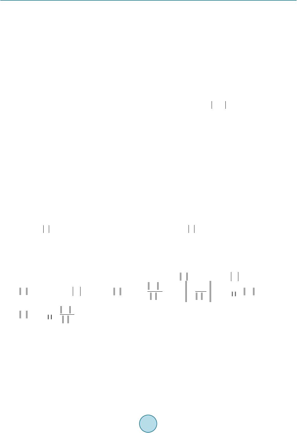

M. M. Tabanjeh

465

vex hulls, Voronoi diagrams, testing whether the line intervals of a given family have nonempty common inter-

section, and finding the orientation of a high dimensional polyhedron. We refer the reader to [1]-[5], and to the

bibliography therein for earlier work. These applications have motivated extensive algorithmic work on compu-

ting the value and particulary the sign of the determinant. One of the well-known numerical algorithms is

Clarkson’s algorithm. In [6], Clarkson uses an adaption of Gram-Schmidt procedure for computing an ortho-

gonal basis and employs approximate arith metics. His algo rithm runs in time

( )

Odb

and uses

2 1.5bd

bits

to represent the values for a d × d determinant with b-bit integer entries. On the other hand, the authors of [7]

proposed a method for evaluating the signs of the determinant and bounding the precision in the case where

3n≤

. Their algorithm asymptotic worst case is worse than that of Clarkson. However, it is simpler and uses re-

spectively b and

()

-bit arithmetic. In this paper we examine two different approaches of computing the de-

terminant of a matrix or testing the sign of the determinant; the numerical and the algebraic approach. In partic-

ular, numerical algorithms for computing various factorizations of a matrix A which include the orthogonal fac-

torization

A QR=

and the triangular factorizations

A LU=

AP LU=

, and

AP LUP=

seem to be the

most effective algorithms for computing the sign of

( )

det A

provided that

det A

is large enough relative to

the computer precision. Alternatively, the algebraic techniques for computing

det A

modulo an integer M

based on the Chinese remainder theorem and the p-adic lifting for a prime p use lower precision or less arith-

metic operations. In fact, the Chinese remainder theorem required less arithmetic operations than the p-adic lift-

ing but with higher precision due to (9). We also demonstrate some effective approaches of combining algebraic

and numerical techniques in order to decrease the precision of the computation of the p-adic lifting and to intro-

duce an alternative technique to reduce the arithmetic operations. If

det A

is small, then obtaining the sign of

the determinant with lower precision can be done by effective algebraic methods of Section 4. Although, the

Chinese remainder algorithm approach requires low precision computations provided that the determinant is

bounded from above by a fixed large number. This motivated us to generalize to the case of any input matrix A

and to decrease the precision at the final stage of the Chinese remaindering at the price of a minimal increase in

the arithmetic cost. Furthermore, in Section 5 we extend the work to an algorithm that computes

( )

det modAM

using low precision by relying on the p-adic lifting rather than the Chinese remaindering.

2. Definitions, Basic Facts, and Matrix Norms

Definition 1. For an n × n matrix A, the determinant of A is given by either

( )( )

( )

det1det, for1,,,

ij ij

AAa Ain

==−=

∑



( )()

( )

det1det, for 1,,,

ij ij

AAa Ajn

==−=

∑



where

()

1n−

-by-

( )

1n−

matrix obtained by deleting the i-th row and j-th column of A.

Fact 1. Well-known properties of the determinant include

()( )( )

detdet detABA B=

()

( )

det detAA=

and

()( )

det det

cA cA=

for any two matrices

∈

and

c∈

Definition 2. If A is a triangular matrix of order n, then its determinant is the product of the entries on the

main diagonal.

Definition 3. For a matrix A of size m × n, we define 1-norm:

1max m

j nij

≤≤ =

=∑

∞

-norm:

max

i mij

≤≤ =

∞

∑

, p-norms:

00 1

sup supmax

xx x

Ax x

AA Ax

≠≠ =





= ==





, and 2-norm:

= max

≠

3. Numerical Computations of Matrix Determinant

We find the following factorizations of an n × n matrix A whose entries are either integer, real, or rational by

Gaussian elimination.

A LU=

(1)

AP LU=

(2)

AP LUP=

(3)

We reduce A to its upper triangu lar form U. The matrix L is a unit lower triangular whose diagonal entries are

M. M. Tabanjeh

466

all 1 and the remaining entries of L can be filled with the negatives of the multiples used in the elementary op er-

ations. Pr is a permutation matrix results from row interchange and Pc is a permutation matrix results from col-

umn interchange.

Fact 2. If P is a permutati on matrix, then

det 1P= ±

. Moreover,

det 1I=

, where I is an identity matrix.

3.1. Triangular Factorizations

The following algorithm computes

( )

det A

or its sign based on the fa c torizations (1)-(3).

Algorithm 1. Triangular factorizations.

Input: An n × n matrix A.

Output:

( )

det A

Computations:

1) Compute the matrices L, U satisfying Equation (1), or Pr, L, U satisfying Equation (2), or Pr, L, U, Pc

satisfying Equation (3).

2) Compute

det L

detU

for Equation (1), or

det

det L

detU

for Equation (2), or

det

det L

detU

det

for Equation (3).

3) Compute and output

( )()

detdet detA LU=

for Equation (1), or

()( )( )

detdetdet det

AP LU

for Eq-

uation (2), or

( )()()()

( )

detdetdet detdet

APLU P=

for Equation (3).

One can easily output the sign of

det A

from the above algorithm. We only need to compute the sign of

det

det L

detU

, and

det

at stage 2 and multiply these signs. The value of

det

and

det

can be

easily found by tracking the number of row or column interchanges in Gaussian elimination process which will

be either 1 or −1 since those are permutation matrices. As L is a unit lower triangular matrix,

det 1L=

. Finally,

the computations of

detU

required

1n−

multiplications since U is an upper triangular matrix. Therefore, the

overall arithmetic operations of Algorithm 1 will be dominated by the computational cost at stage 1, that is,

( )()

12 1

nn ni

−

−−

∑

multiplications, the same number for additions, subtractions, and comparisons, but

( )

nn i

−

−=

∑

divisions. However, Algorithm 1 uses

−

∑

comparisons to compute (2) rather than

−

∑

3.2. Orthogonal Factorization

Definition 4. A square matrix Q is called an orthogonal matrix if

T.QQ I=

Equivalently,

−=

, where

QT is the transpose of Q.

Lemma 1. If Q is an orthogona l matrix, then

( )

det 1Q= ±

Proof. Since Q is orthogonal, then

QQ I=

. Now

T1QQ I= =

and thus

1QQ =

, but

QQ=

which implies that

1QQ Q==

, hence

1Q= ±

Definition 5. If

∈

, then there exists an orthogonal matrix

Q×

∈

and an upper triangular matrix

∈

so that

.A QR=

(4)

Algorithm 2. QR-factorization.

Input: An n × n matrix A.

Output:

( )

det A

Computations:

1) Compute an orthogonal matrix Q satisfying the Equation (4).

2) Compute

detQ

3) Compute the matrix

( )

T,ij

R QAr= =

4) Compute

( )()

det detii

A Qr

=∏

, where

are the main diagonal entries of R.

Here, we consider two well-known effective algorithms for computing the

factorization; the House-

holder and the Given algorithms. The Householder transformation (or reflection) is a matrix of the form

2HI=− vv

where

1=v

Lemma 2. H is symmetric and orthogonal. That is,

HH=

and

.HHI⋅=

Proof.

2,HI=− vv

and since

II=

and

( )

,=vv vv

then

( )

TT TT

2 2.HII H=− =−=vv vv

Hence,

M. M. Tabanjeh

467

H is symmetric. On the other hand,

( )( )()

TTTTTTT T

224444.HH IIIvII=−− =−+=−+=vvvvvvv vvvvvv

Therefore, H is orthogonal, that is,

−=

The Householder algorithm computes

−

=∏

as a product of

n−

matrices of Householder trans-

formations, and the upper triangular matrix

QA R=

Lemma 3.

( )()

det1n

Q−

= −

for a matrix Q computed by the Househol de r algorit h m.

Proof. Since

i ii

HI=− vv

for vectors

1, ,1in= −

, Lemma 2 implies that

HH I=

and hence

()

det 1

. Notice that

( )

det 21I−=−ee

where

( )

1,0,,0e=

. Now for

01t≤≤

, we define the trans-

formation

()

( )

11i

vttvee

= −+

. Then the function

( )( )()

( )

detDtIvtvt= −

is continuous and

1D=

t∀

Hence

( )

1 det21DI vv=−=−

since

1=v

and

( )

()

0 det21DIee=−=−

. This proves that

det 1

H= −

i∀

. But

−

=∏

, we have

( )

det 1

−

= −

The Givens rotations can also be used to compute the QR factorization, where

QG G=

, t is the total

number of rotations, Gj is the the j-th rotation matrix, and

QA R=

is an upper triangular matrix. Since the

Givens algorithm computes Q as a product of the matrices of Givens rotations, then

( )

det 1Q=

. We define

()( )

ii kk

G WcsWcsc= ==

,,ik ki

GWWs= =−=

for two fixed integers i and k, and for a pair of nonzero rea l

numbers c and s that satisfies

such that

GG I=

. If the Householder is used to find the QR, Algo-

rithm 2 uses

1n−

multiplications at stage 3. It involves

( )

3n On+

multiplications at stage 1, and

()

evaluations of the square roots of positive numbers. If the Givens algorithm is used to find the QR, then it in-

volves

()

2n On+

multiplications at stage 3,

()

n On

multiplications at stage 1, and

( )

evalua-

tions. This shows some advantage of the Householder over the Givens algorithm. However, the Givens rotations

algorithm allows us to update the QR of A successively by using only

( )

O kn

arithmetic operations and

square root evaluations if

( )

rows or columns of A are successively replaced by new ones. Therefore, in

this case, the Givens algorithm is more effective.

4. Algebraic Computations of Matrix Determinant

4.1. Determinant Computation Based on the Chinese Remainder Theorem

Theorem 1. (Chinese remainder theorem.) Let

, ,,

mm m



be distinct pairwise relatively prime integers

such that

mm m> >> >



(5)

Let

∏

, and let D denote an integer satisfying th e inequality

0.DM≤<

(6)

Let

( )

mod .

rD m=

(7)

( )( )

, mod , 1mod , 1,,.

iiii iii

Ms Mmysmik

= ≡≡∀=

(8)

Then D is a unique integer satisfying (6) and (7). In additio n,

( )

mod .

ii i

D MryM

=∑

(9)

Algorithm 3. (Computat i on of

( )

detmod AM

based on the Chinese remainder theorem.)

Input: An integer matrix A, an algorithm that computes

( )

detmod Am

for any fixed integer

, k in-

tegers

mm

satisfying (5) and are pairwise r elatively prime, and

12 k

M mmm=

Output:

( )

detmod AM

Computations:

1) Compute

( )

detmod

r Am=

1, ,ik=

2) Compute the integers Mi, si, and yi as in (8)

1,,ik∀=

3) Comput e an d output D as in (9).

M. M. Tabanjeh

468

The values of yi in (8) are computed by the Euclidean algorithm when applied to si and mi for

1, ,ik=

Algorithm 3 uses

( )

O kn

arithmetic operations (ops) at stage 1,

( )

log loglogOk mm

ops at stage 2, and

( )

log

Ok k

ops at stage 3. The computations of the algorithm are performed with precision of at most

log m





bits at stage 1, and at most

log M





bits at stages 2 and 3. The latest precision can be decreased at

the cost of slightly in creasing the arithmetic operations [8].

Lemma 4. For any pair of integers M and d such that

Md>

, we have

( )( )( )

mod if m od , and mod otherwise.

ddM dMddMM= <=−

(10)

Suppose that the input matrix A is filled with integers and an upper bound

det

dA≥

is known. Then we

may choose an integer M such that

Md>

and compute

( )

detmod AM

. Hence,

det A

can be recovered

by using (10).

4.2. Modular Determinant

Let

A×

∈

and

( )

detdA=

. In order to calculate

( )

detmod Ap

, we choose a prime p that is bigger than

and perform Gaussian elimination (2) on

( )

mod

∈

. This is the same as Gau s s ian elimination over



, except that when dividing by a pivot element a we have to calculate its inverse modulo p by the ex-

tended Euclidean algorithm. This requires

( )

3n On+

arithmetic operations modulo p. On the other hand, if

we need to compute

( )

detmod Ap

for the updated matrix A, we rely on the QR factorization such that

( )()

modA QRp=

and

( )

modQQ Dp=

, where D is a diagonal matrix and R is a unit upper triangular matrix.

The latest factorization can be computed by the Givens algorithm [9]. If the entries of the matrix A are much

smaller than p, then we do not need to reduce modulo p the results at the initial steps of Gaussian elimination.

That is, the computation can be performed in exact rational arithmetics using lower precision. In this case, one

may apply the algorithm of [10] and [11] to keep the precision low. The computations modulo a fixed integer

1M>

can be performed with precision

log M





bits. In such a computation, we do not need to worry about

the growth of the intermediate values anymore. However, to reduce the cost of the computations, one can work

with small primes modular instead of a large prime, that is, these primes can be chosen very small with loga-

rithmic length. Then the resulting algorithm will have lower cost of

( )

O nk

and can be performed in parallel.

Now, one can find a bound on the

det A

without actually calculating the determinant. This bound is given by

Hadamard’s inequality which says that

()

det ,

Anaa n

≤=

(11)

where

max

i jnij

≤≤

= ∈

(nonnegative integers) is the maximal absolute value of an entry of A.

5. Alternative Approach for Computing Matrix Inverses and Determinant

5.1. p-Adic Lifting of Matrix Inverses

In this section, we present an alternative approach for computing matrix determinant to one we discussed in ear-

lier sections. The main goal is to decrease the precision of algebraic computations with no rounding errors. The

technique relies on Newton’s-Hensel’s lifting (p-adic lifting) and uses

( )

logOn n

arithmetic operations.

However, we will also show how to modify this technique to use order of n3 arithmetic operations by employing

the faster p-adic lifting. Given an initial approximation to the inverse, say S0, a well-known formula for New-

ton’s iteration rapidly improves the initial ap proximation to the inverse of a nonsingula r n × n matrix A:

()( )

222, 0.

iiiiiiii

SSIASSS ASIS ASi

=−=− =−≥

(12)

Algorithm 4. (p-adic lifting of matrix inver ses.)

Input: An n × n matrix A, an int ege r

1p>

, the matrix

( )

mod

SA p

−

, and a nat ural number h.

Output: The matrix

( )

mod

−

Computations:

1) Recursively compute the matrix

by the equation,

M. M. Tabanjeh

469

( )

2mod ,where2, 1,,.

jj j

SSIASpJjh

−−

=−==

(13)

2) Finally, outputs

Note that,

( )

mod

SA p

−

j∀

. This follows from the equation

( )

1mod J

I ASI ASp

−

−=−

The above algorithm uses

( )

arithmetic operations performed modulo pJ at the j-th stage, that is, a to tal of

( )

O hn

arithmetic operations with precision of at most

logJp





bits.

5.2. p-Adic Lifting of Matrix Determinant

We can further extend p-adic lifting of matrix inverses to p-adic lifting of matrix determinants, that is

( )

detmod

, using the following formula [12]:

( )

det .

kkk

A−

∏

(14)

Here, Ak denotes the k × k leading principal (north-western) submatrix of A so that

AA=

for

1, ,kn=

Moreover,

( )

,kk

denotes the

( )

,kk

-th entry of a matrix B. In order to use Formula (14), we must have the

inverses of Ak available modulo a fixed prime integer p for all

. A nonsingular matrix A modulo p is called

strongly nonsingular if the inverses of all submatrices Ak exist modulo p. In general, a matrix A is called strongly

nonsingular if A is nonsingular and all k × k leading principle submatrices are nonsingular. Here, we assume that

A is strongly nonsingular for a choice of p. Finally, Algorithm 4 can be extended to lifting

det A

(see Algo-

rithm 5).

Algorithm 5. (p-adic lifting of matrix determinant.)

Input: An integer

1p>

, an n × n matrix A, the matrices

()

mod

SA p

−

, and a natur al number h.

Output:

( )

detmod

Computations:

1) Apply Algorithm 4 to all pairs of matrices

and

0,k

, (replacing the matrices A and

in the algo-

rithm), so as to compute the matrices

( )

mod

hk k

SA p

−

, for

1, ,kn=

2) Compute the value

( )

1mod 2mod .

det

hkkhkkk

pSI ASp

 

= −

 



∏

(15)

3) Compute an d output the va lue

()

detmod

, as the reciprocal of

( )

1mod

det







The overall computational cost of Algorithm 5 at stage 1 is

( )

O hn

arithmetic operations performed with

precision at most

logHp





bits. However, at stage 2, the algorithm uses

( )

operations with precision

2 logHp





bits. At stage 3, only one single multiplication is needed. All the above operations are calculated

modulo p2H. Now, we will estimate the value of H and p that must satisfy the bound

2 det

pA>

. But, due to

Hadamard’s bound (11), we have

()

2 det2

Aanp

which implies that

2logloglog 2

ppp

H nann>+ +

. Therefore, it is suffices to choose p and H satisfying the inequalities

( )

an p<

and

( )

2log2

H aa



>



. In the next section, we will present an alternative faster tech-

nique to computing matrix determinant that uses only

( )

based on the divide-and-conquer algorithm .

Example 1. Let

1 1718

11819.

5 1620





=





Then,

[ ]

1,A=

1 17

1 18

A

=



, and

1 1718

11819.

5 1620





=





By Algorithm 4,

compute the matrices:

[ ]

1,A

−

1817 ,

A−−



=

−



and

56 521

75701.

7469 1

−





= −



−−



Now, we compute

M. M. Tabanjeh

470

[ ]

0,1 1

mod 31,SA

−

= =

0,2 2

mod 3,

−



== 



and

0,3 3

111

mod 3011.

202

−





== 





We apply Algorithm 4

(that is,

( )

0, 0,

2 mod , 2, 1,,

k kkk

SSIASpJjh=−==

) to all pair s of matrices:

( )

[ ]

1,110,110,1

2mod 31,SSSI AS==−=

( )

1,220,22 0,2

2mod 3,

SSSIAS

==−=





and

( )

1,330,33 0,3

7 71

2mod 3671.

2 38

SSSIAS





==−=





We then compute the value

() () ()

[

]

()()( )

2 221

1,11 1,11,22 1,21,331,3

11,12,2 3,3

1,1 2,2 3,3

1mod 222mod 3

det

2243 2783 2510

144 17

12100 2603 2348

1216 1612113 2580 2269

11612269365309 mo

pSIASSIASSIAS

××

= 

=−⋅−⋅−

 

−−−



−−





= ⋅⋅−−−



−−





−−−



=−− =

∏

( )

d 8180.=

Therefore, we output the value of

()

221

detmod 31

××

= −

, since

180 mod 81−≡

5.3. Faster p-Adic Lifting of the D eterminant

Assuming A is strongly nonsingular modulo p, block Gauss-Jordan elimination can be applied to the block 2 × 2

matrix

AEG



=



to obtai n the we ll-known bl ock factorization of A:

IO BOI BC

AEBIO SOI

−



 

=

 

 

where

SGEB C

−

= −

is the Schur complement of B in A. The following is the divide-and-conquer algorithm

for computing

()

det A

Algorithm 6. (Computing the determinant of a strongly nonsingular matrix .)

Input: An n × n stron gl y nonsingul ar matrix A.

Output:

( )

det A

Computations:

1) Partition A according to the block factorization above, where B is an





matrix. (

⋅





refers to

the floor of

.) Compute

−

and S using the matrix equation

SGEB C

−

= −

2) Compute

( )

det B

and

( )

det S

3) Comput e an d output

( )()

detdet detABS=

Since A is strongly nonsingular modulo p, we can compute the inverse of k × k matrix by

( )

logOkH Ik=

arithmetic operations using Algorithm 4. From the above factorization of A, we conclude

that

( )

( )()( )

2 22Dn DnDnIn≤++

 

 

. The computational cost of computing the determinant is

( )

logDn OnH=

. This can be derived from the above factorization of A using recursive factorization ap-

plied to B and S and the inverses modulo

. Here,

( )

is the cost of computing the inverse and

( )

M. M. Tabanjeh

471

the cost of computing the determinant.

6. Improving the Precision of the p-Adic Lifting Algorithm

Definition 6. Let e be a fixed integer such that

log e

where β is the computer precision. Then any integer

z, such that

01ze≤≤−

, will fit the computer pre cision and will be called sh ort integer or e-integer. The integ-

ers that exceed

−=

will be called long integers and we will associate them with the e-polynomials

( )

p xpx

=∑

≤<

for all i.

Recall that Algorithm 4 uses

logjp





bits at stage j. For large j, this value is going to exceed β. In this

section we decrease the precision of the p-adic algorithm and keep it below β. In order to do this, we choose the

base

where K is a power of 2,

2KH≤

, K divides

, and

log .

αβ



≤<





(16)

Now, let us associate the entries of the matrices

mod

and

mod

−

with the e-polynomials in x

for

and for all j and k. These polynomials have degrees

()

1JK−

and take values of the entries for

xe=

. Define the polynomial matrices

( )

mod

jk k

AeA p=

and

( )

mod

jk jk

SeS p=

. Then for

JK≥

, we

associate the p-adic lifting step of (13) with the matrix polynomial

( )()()()( )

( )

,1,1,,1,

2mod .

jkjnjnjn jn

SxSxSxAxSx x

−− −

= −

(17)

The input polynomial matrices a re

()

1,jn

−

and

()

for

1, 2,,jh=

. We perform the computations

in (17) modulo

. The idea here is to apply e-reduction to all the entries of the output matrix polynomial

followed by a new reduction modulo

. The resulting entries are just polynomials with integer coefficients

ranging between

−

and

1e−

. This is due to the recursive e-reductions and then taking modular reductions

again. Note that the output entries are polynomials with coefficients in the range

−

for

≤

even

before applying the e-reductions. This shows that the β-bit precision is sufficient in all of the computation s due

to (16). The same argument can be applied to the matrices

,jk

for all j and

kn<

7. Numerical Implementation of Matrix Determinant

In this section we show numerical implementation of the determinant of n × n matrices based on the triangular

factorization LU, PrLU, and PrLUPc. Algorithm 1 computes the triangular matrices

LLE=+



and

UUE= +



, the permutation matrices



and



, where EL and EU are the perturbations of L and U. In gener-

al, we can assume that

PP=



and

PP=



since the rounding error is small.

Definition 7. Let

, ,

APAP LUAE

−−

′ ′′

= −=

 

(18)

and let

e′

, a,



, and



denote the maximum absolute value of the entries of the matrices

E′

, A,



, and



. Also,

E′

is the error matrix of the order of the roundoff in the entries of A.

Assuming floating point arithmetic with double precision (64-bits) and round to

-bit. Then the upper

bound on the magnitude of the relative rounding errors is

−

=

, where



is the machine epsilon. Our goal is

to estimate

e′

Theorem 2. ([13]) F or a m atrix

( )

,ij

Aa=

, let

denote the matrix

( )

,ij

. Then unde r (18),

( )

,EA LU

′′

≤+



and

( )

.eea nlu

′≤=+





(19)

From the following matrix norm property

1max

ijij

A aA

 ≤≤





, for

1, 2,q= ∞

, we obtain the bound

.eE

∞

′′

≤

Theorem 3. Let

denotes the maximum absolute value of all entries of the matrices

( )

computed by

Gaussian elimination, which reduces

A′

to the upper triangular form and let



as define d above. Then

M. M. Tabanjeh

472

( )

21.8 .

eeEnaan+

+∞

′′

≤= ≤<

(20)

By using the following results, we can estimate the magnitude of the perturbation of

det A

and

det A′

caused by the pe rturbati on of

A′

. Here we assume that

PPIAA

′

= ==

and write,

( )

, detdet.

eeeAE A

′

= =+−

(21)

We use the following facts to estimate

of (21) in Lemma 5 below.

Fact 3.

det

≤

1, 2,q= ∞

BA≤

1,q=∞

, if

≤

;

≤

1, 2,q= ∞

, if B is a

submatrix of A.

A EAne+≤ +

, for

1, 2,q= ∞

;

A EAne+≤ +

Lemma 5.

( )

12, f or 1,2,.

eAneneq

−

≤+ =∞

Combining Lemma 5 with the bound (19) enables us to extend Algorithm 1 as follows:

Algorithm 7. (Bounding de t erminant.)

Input: An

nn×

real matrix A and a positive



Output: A pair of real numbers

−

and

such that

det .d Ad

−+

≤≤

Computations:

1) Apply Algorithm 1 in floating po int arithmetic with unit roundoff bounded by



. Let

UUE

= +



denote

the computed upper triangular matrix, approximating the factor U of A from (2) or (3).

2) Compute the upper bound

of (20) where

′

3) Substitute e+ for e and

( )

min|,, AAAA

∞∞







for

in Lemma 5 and obtain an upper bound

4) Output the values

det

d Ue

−

= −



and

det

d Ue

= +



Example 2. Let

5 31

036 01.6667 5.1667

19 3164.7500 1.50003.2000 .

42 53.4000 5.25001.3333

17 2112

54 9



−

 −





=≈









Using Matlab, Gaussian elimination

with complete pivoting gives the matrix U rounded to 4 bits:

5.2500 1.33333.4000

05.5899 1.0794

00 3.2342





= −−





1 00

0.3175 1 0

0.28570.5043 1





=



−



UUE= +



LLE= +



where EU and EL are the matrices obtained from accu-

mulation of rounding errors. Also

001

100

010





=





, and

001

1 0 0.

010





=





Then

06 106 10

00 0

003 10

−−

′

−



××



=





is a perturbation in A, and

1.2 10

E−

′∞= ×

. We now compute the upper bound

of (20). Therefore,

62.9618ee

′≤≤

, where

5.25

is the maximum of

,ij

of A, l = 1 is th e ma x imu m o f

of L,

−

=

, and

3n=

is the size of the input matrix

. Hence we obtain the following upper bound

by Lemma 5. That is,

( )

127

min,,2.2347 10

eAAAAnene

−

∞∞



≤ +=×





, where

9.7A=

9.9833A∞=

, and

9.8406AA

∞

. Hence,

2.2347 10

= ×

is an upper bound of

det2.2347 10

d Ue

−

= −=−×



and

det2.2347 10

d Ue

+= +=×



. Since

( )

det 94.91597A= −

, we have

M. M. Tabanjeh

473

( )

det det

UeA Ue

− ≤≤+



. On the other hand

()( )

detdet 0.00123

eA EAA

= +−=

which is less than the

upper bound

2.2347 10×

we have computed.

Acknowledgements

We thank the editor and the referees for their valuable comments.

References

[1] Muir, T. (1960) The Theory of Determinants in Historical Order of Development. Vol. I-IV, Dover, New York.

[2] Fortune, S. (1992) Voronoi Diagrams and Delaunay Triangulations. In: Du, D.A. and Hwang, F.K., Eds., Computing in

Euclidean Geometry, World Scientific Publishing Co., Singapore City, 193-233.

[3] Brönnimann, H., Emiris, I.Z., Pan, V.Y. and Pion, S. (1997) Computing Exact Geometric Predicates Using Modular

Arithmetic. Proceedings of the 13th Annual ACM Symposium on Computational Geometry, 174-182.

[4] Brönnimann, H. and Yvinec, M. (2000) Efficient Exact Evaluation of Signs of Determinant. Algorithmica, 27, 21-56.

http://dx.doi.org/10.1007/s004530010003

[5] Pan, V.Y. and Yu, Y. (2001) Certification of Numerical Computation of the Sign of the Determinant of a Matrix. Algo-

rithmica, 30, 708-724. http://dx.doi.org/10.1007/s00453-001-0032-8

[6] Clarkson, K.L. (1992) Safe and Effective Determinant Evaluation. Proceedings of the 33rd Annual IEEE Symposium

on Foundations of Computer Science, IEEE Computer Society Press, 387-395.

[7] Avnaim, F., Boissonnat, J., Devillers, O., Preparata, F.P. and Yvinec, M. (1997) Eval uating Signs of Determinants Us-

ing Single-Precision Arithmetic. Algorithmica, 17, 111-132. http://dx.doi.org/10.1007/BF02522822

[8] Pan, V., Yu, Y. and Stewart, C. (1997) Algebraic and Numerical Techniques for Computation of Matrix Determinants.

Computers & Mathematics with Applications, 34, 43-70. http://dx.doi.org/10.1016/S0898-1221(97)00097-7

[9] Golub, G.H. and Van Loan, C.F. (1996) Matrix Computations. 3rd Edition, John Hopkins University Press, Baltimore.

[10] Edmonds, J. (1967) Systems of Distinct Representatives and Linear Algebra. Journal of Research of the National Bu-

reau of Standards, 71, 241-245. http://dx.doi.org/10.6028/jres.071B.033

[11] Bareiss, E.H. (1969) Sylvester’s Identity and Multistep Integer-Preserving Gaussian Elimination. Mathematics of

Computation, 22, 565-578.

[12] Bini, D. and Pan, V.Y. (1994) Polynomial and Matrix Computations, Fundamental Algorithms. Vol. 1, Birkhäuser,

Boston. http://dx.doi.org/10.1007/978-1-4612-0265-3

[13] Conte, S.D. and de Boor, C. (1980) Elementary Numerical Analysis: An Algorithm Approach. McGraw-Hill, New

York.