LQG Control Design for Balancing an Inverted Pendulum Mobile Robot

doi:10.4236/ica.2011.22019

Paper Menu >>

Journal Menu >>

Intelligent Control and Automation, 2011, 2, 160-166

doi:10.4236/ica.2011.22019 Published Online May 2011 (http://www.SciRP.org/journal/ica)

LQG Control Design for Balancing an Inverted Pendulum

Mobile Robot

Ragnar Eide, Per Magne Egelid, Alexander Stamsø, Hamid Reza Karimi

Department o f En g i neer i n g , Faculty of Engineering and Science, University of Agder,

Grimstad, Norway

E-mail: [email protected]

Received December 26, 2011; revised May 17, 2011; acce pted May 19, 2011

Abstract

The objective of this paper is to design linear quadratic controllers for a system with an inverted pendulum

on a mobile robot. To this goal, it has to be determined which control strategy delivers better performance

with respect to pendulum’s angle and the robot’s position. The inverted pendulum represents a challenging

control problem, since it continually moves toward an uncontrolled state. Simulation study has been done in

MATLAB Simulink environment shows that both LQR and LQG are capable to control this system success-

fully. The result shows, however, that LQR produced better response compared to a LQG strategy.

Keywords: LQG Control, Inverted Pendulum, Mobile Robot

1. Introduction

Inverted pendulum has been the subject of numerous

studies in automatic control since the forties. The in-

verted pendulum is a typical representative of a class of

high-order nonlinear and non-minimum phase systems

[1]. Since the system is inherently nonlinear, it is useful

to illustrate some of the ideas in nonlinear control.

Wheeled mobile robots have in the recent years

become increasingly important in industry, since they

provide a large degree of flexibility and efficiency with

respect to transportation, inspection, and operation. In

many cases, however, it is the control, or lack of

knowledge in control, which limit the area of applicatio n .

In this system, an inverted pendulum is attached to a

robot equipped with a motor that drives it along a

horizontal track (robot will in the following mean an

autonomous robot provided with the Robotics Starter Kit

from National Instruments). The user is able to dictate

the position and velocity of the robot through the motor.

The pendulum is characterized by an unstable equi-

librium point, and its behavior can be used in the analysis

and stability control of many similar systems.

Many different control methods are proposed for the

inverted pendulum problem. The Proportional-Integral-

Derivative (PID) and Proportional-Derivative (PD)

controllers [2] and [3], Model Predictive Control (MPC)

[4], and fuzzy contr ol [5] to mentio n a few. How ever one

of the obstacles by using the PID and PD controllers are

that they alone cannot effectively control all of the

pendulum state variables (modes) since they are of lower

order than the pendulum itself. Hence, they are usually

replaced by a full-order controller [3]. A linear state

feedback controller based on the linearized inverted

pendulum model can instead be used, and may also be

extended with a disturbance observer (Kalman filter) to

improve the disturbance rejection performance.

The proposed method is to balance an inverted pen-

dulum placed on top of a mobile robot by use of LQR/

LQG control methods. Our solution implements an LQG

controller with comparison to a simple LQR controller.

The controller found by means of a more analytical

approach will be tested with implementation of the

controller in the MATLAB/Simulink environment.

With varying input forces the goal is to design a

controller capable of meeting the following requirements:

 settling time,

T, less than 5 seconds

 maximum overshoot of 10 degrees (0.175 radians)

 rise time T less than 0.5 s

We will in part one describe a simplified mathematical

model of the problem. Then, when having a state space

model of the system, we can in part two go on and

determine the controllers and observers. Finally, the

results from simulations will then be presented and

compared in part three.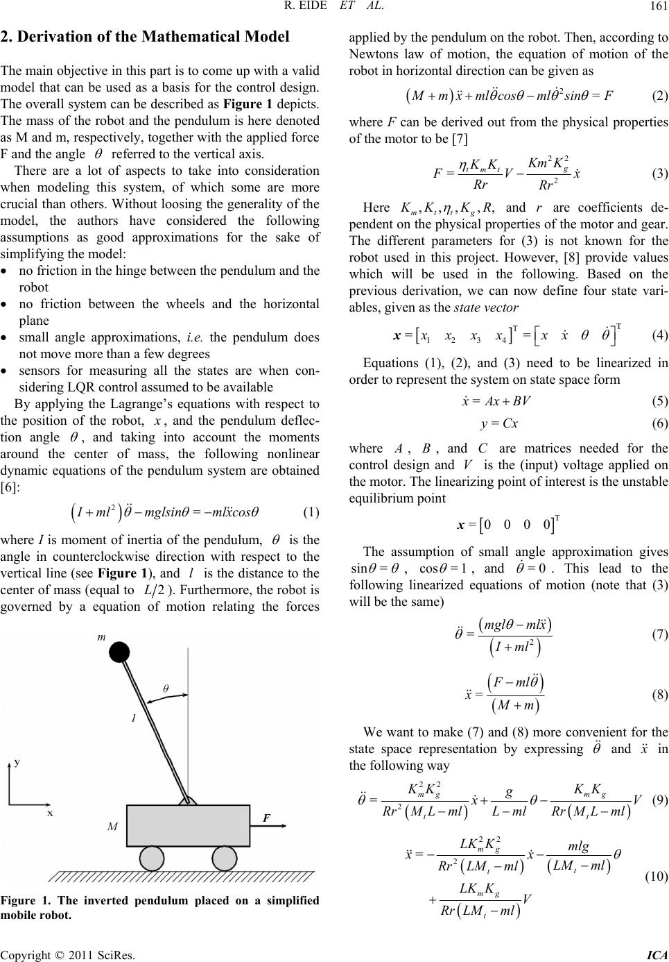

R. EIDE ET AL.161

2. Derivation of the Mathema tical Mode l

The main objective in this part is to come up with a valid

model that can be used as a basis for the control design.

The overall system can be described as Figure 1 depicts.

The mass of the robot and the pendulum is here denoted

as M and m, respectively, together with the applied force

F and the angle



referred to the vertical axis.

There are a lot of aspects to take into consideration

when modeling this system, of which some are more

crucial than others. W ithout loosing the generality of the

model, the authors have considered the following

assumptions as good approximations for the sake of

simplifying the model:

 no friction in the hinge between the pendulum and the

robot

 no friction between the wheels and the horizontal

plane

 small angle approximations, i.e. the pendulum does

not move more than a few degrees

 sensors for measuring all the states are when con-

sidering LQR control assumed to be available

By applying the Lagrange’s equations with respect to

the position of the robot,

, and the pendulum deflec-

tion angle



, and taking into account the moments

around the center of mass, the following nonlinear

dynamic equations of the pendulum system are obtained

[6]:



mlmglsin mlxcos



 

 



(1)

where I is moment of inertia of the pendulum,



is the

angle in counterclockwise direction with respect to the

vertical line (see Figure 1), and is the distance to th e

center of mass (equal to l

2L). Furthermore, the robot is

governed by a equation of motion relating the forces

Figure 1. The inverted pendulum placed on a simplified

mobile robot.

applied by the pendulum on the robot. Then, according to

Newtons law of motion, the equation of motion of the

robot in horizontal direction can be given as





mx mlcosmlsinF

 

 

 

 (2)

where F can be derived out from the physical properties

of the motor to be [7]

tmtKm K

Rr Rr





x (3)

Here ,,, ,,

mttg

KKR



and are coefficients de-

pendent on th e physical properties of th e motor and gear .

The different parameters for (3) is not known for the

robot used in this project. However, [8] provide values

which will be used in the following. Based on the

previous derivation, we can now define four state vari-

ables, given as the state vector



1234

==xxxx xx









x (4)

Equations (1), (2), and (3) need to be linearized in

order to represent the system on state space form

Ax BV



 (5)

Cx (6)

where

, , and are matrices needed for the

control design and is the (input) voltage applied on

the motor. The linearizing point of interest is the unstable

equilibrium point



=0000x

The assumption of small angle approximation gives

sin =



, cos =1



, and . This lead to the

following linearized equations of motion (note that (3)

will be the same)











=mgl mlx

Iml









 (7)















 (8)

We want to make (7) and (8) more convenient for the

state space representation by expressing



 and

 in

the following way

 

=mg mg

KK KK

Lml RrMLml

RrM Lml









  (9)



LK Kmlg

LM ml

Rr LMml

LK KV

Rr LMml









 

(10)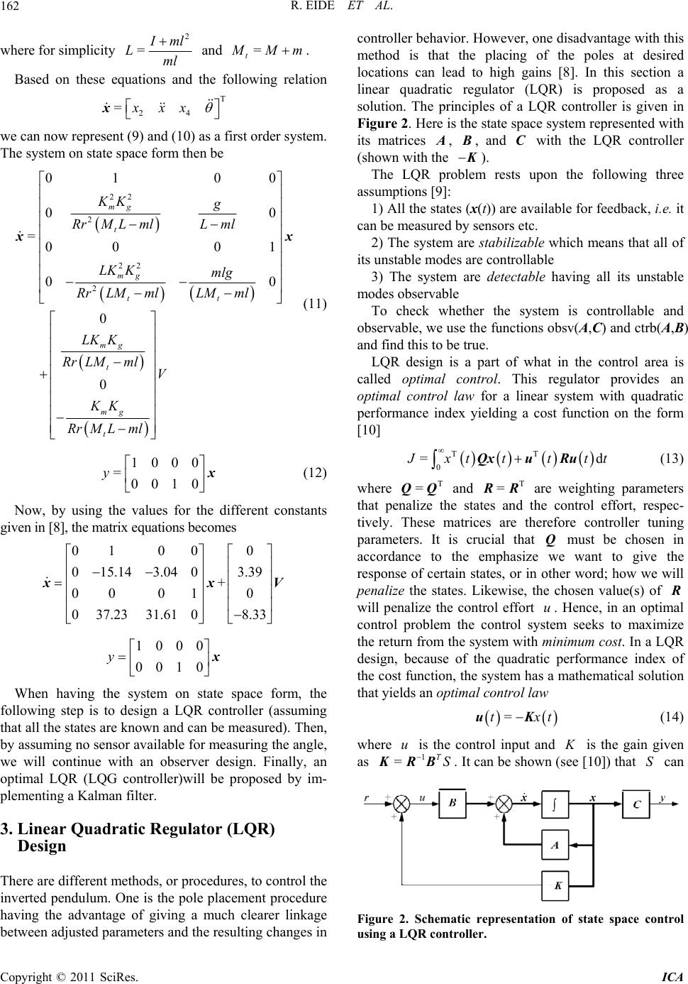

R. EIDE ET AL.

162

where for simplicity 2

Lml

 and =



Based on these equations and the following relation

=xxx











we can now represenfirst

The system on state sen be

t (9) and (10) as a order system.

pace form th



01 00



KK g

LK Kmlg

LM ml

Rr LMml

LK K

Rr LMmlV

RrMLml



































(11)

(12)

Now, by using the values for the different constants

given in [8], the matrix equations becomes





When having the system on state space form, the

following step is to design a LQR controller (assuming

that all the states are known and can be measured). Then,

by assuming no sensor available for msuring the angle,

we will continue with an observer dsign. Finally, an

placement procedure

nkage

es in

covior. However, one disadvantage with this

ethod is that the placing of the poles at desired

=00 01

tLm

RrM Lml









1000

=0010

y





01 000

0 15.14 3.040

00 010













3.39

+



037.2331.61 08.33







1000

0010

y





timal LQR (LQG controller)will be proposed by im-

plementing a Kalman filter.

3. Linear Quadratic Regulator (LQR)

Design

There are different methods, or procedures, to control the

nverted pendulum. One is the pole i

having the advantage of giving a much clearer li

between adjusted parameters and the resulting ch ang

ntroller beha

locations can lead to high gains [8]. In this section a

linear quadratic regulator (LQR) is proposed as a

solution. The principles of a LQR controller is given in

Figure 2. Here is the state space system represented with

its matrices

, B, and C with the LQR controller

(shown with the



The LQR problem rests upon the following three

assumptions [9]:

1) All the states (x(t)) are available for feedback, i.e. it

can be measured by sensors etc.

2) The system a stabiliz ble which means that all of

its unstable modee cont

re a

s arrollable

bsv(A,C) and ctrb(A,B)

an the control area is

ca for a linear system with quadratic

3) The system are detectable having all its unstable

modes observable

To check whether the system is controllable and

observable, we use the functions o

d find this to be true.

LQR design is a part of what in

lled optimal control. This regulator provides an

optimal control law

rformance index yielding a cost function on the form

[10]

 

xt tttt

Qxu Ru (13)

where T

=QQ and T

=RR are weighting parameters

that penalize the states and the control effort, respec-

tively. These matrices are therefore controller tuning

parame



ters.

nce to

se of certain

e the st

It is cru must be chosen in

accorda the want

responr word;

cial that

emphasize we

states, or in

otheto give the

how we will

penaliz ates. Likewise, the chosen value(s) of R

will penalize the control effort u. Hence, in an optimal

control problem the control system seeks to maximize

the return from the system with mnimum cost. In a LQR

design, because of the quadratic performance index of

the cost function, the system has a mathe matical solution

that yields an optimal control law





=txtuK (14)

where u is the control input and K is the gain given

as 1

=TS



RB . It can be shown (see [10]) that S can



Figure 2. Schematic representation of state space control

using a LQR controller.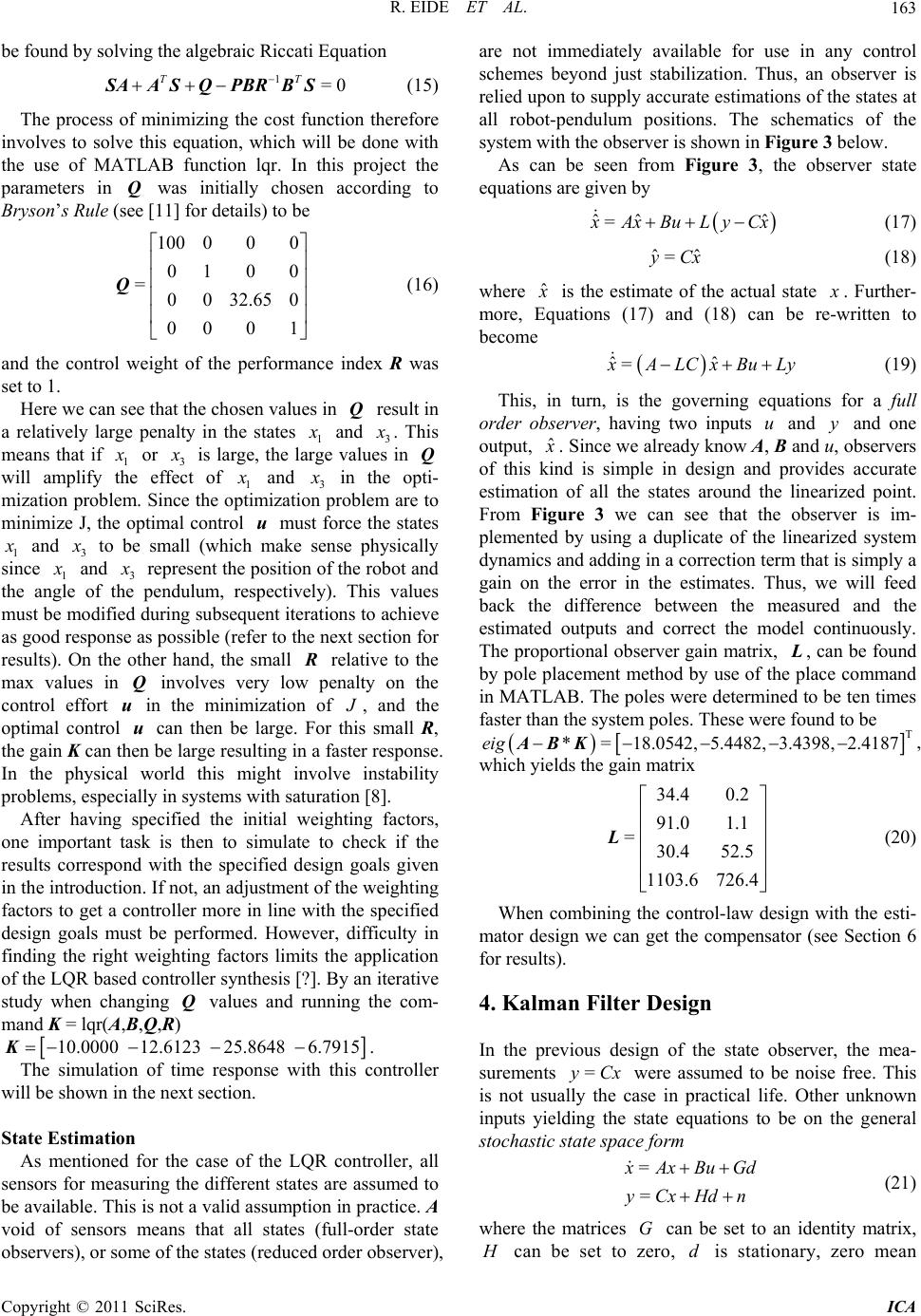

R. EIDE ET AL.163

be found by solving the algebraic Riccati Equation

(15)

The process of minimizing the cost function therefore

involves to solve this equation, which will be done with

the use of MATLAB function lqr. In this project the

parameters in was initially chosen according to



1=0

TT

SAA SQPBRBS

Bryson’s Rule (see [11] for details) to be

100



000

01 0 0





=0032.650



00 0 1





and the control weight of the performance index R was

set to 1.

Here we can see that the chosen values in Q result in

a relatively large penalty in the states

(16)

and 3

. This

means that if 1

or 3

e effect

is large, the

will amplify ofe largvalues in Q

th 1

and 3

in the opti-

n problem are to mization proble.he izat

minimize J, the optim contm

m Since t

al optim

rol io

ust forc

u e the states

and 3

to be small (which makesysically sene ph

since 1

and 3

represent the position of the robot and

the angle of the pendulum

,ectively). Tha respis vlues

must be modified during subsequent iterations to achieve

as good response as possible (refer to thext section for

results). On the other nd, the small e n

relative to t

max values in Q involves vy lowenalty on the

control effort u in the minimization of

er p

, and the

optimal control u can then be rge. For this small R,

e gain Kcan then be large resulting in a faster response.

In thephysical world this might involve instability

problems, especially in systems with saturation [8].

After having specified the initial weighting factors,

one important task is then to simulate to check if the

results correspond with the specified dign goals given

in the introduction If not, an ad justment o f the weigh ting

factors to get a controller more in line with te specified

design goals must be performed. However, difficulty in

finding the right weighting factors limits the application

of the LQR based controller synthesis [?]. By an iterative

study when changing Q values and running the

com-

mand K = lqr(A,B,Q,R)





10.0000 12.6123 25.8648 6.7915 K.

The simulation of time response with this controller

will be shown in the next section.

State Estimation

As mentioned for the case of the LQR controller, all

sensors for measuring the different states are assumed to

be available. This is not valid assumption in practice. A

are not immediately avai

void of sensors means that all states (full-order state

observers), or some of the states (reduced order observer),

lable for use in any control

schemes beyond just stabilization. Thus, an observer is

re e schematics of the

stem with the observer is shown in Figure 3 below.

from Figure 3, the observer state

lied upon to supply accurate estimations of the states at

all robot-pendulum positions. Th

syAs can be seen

uations are g i v en by



ˆˆ ˆ

AxBuL yCx 

 (17)

ˆˆ

=yCx

(18)

where ˆ

is the estimate of the actual state

. Further-

more, Equations (17) and (18) can be re-written to

become





ˆˆ

ALCxBuLy





 (19)

This, in turn, is the governing equations for a full

order observer, having two inputs u and y and one

output, ˆ

. Since we already know and servers

of this ki is simple in design a

estimation of all the states around t

From 3 we can se

difference between the mea

estimauts and correct the mde

A, B

u, ob

Figure

ted outp

provides accurate

he linearized point.

e that the observer is im-

plemented by using a duplicate of the linearized system

dynamics and adding in a correction term that is simply a

gain on the error in the estimates. Thus, we will feed

back the sured and the

l continuously.

e proportional observer gain matrix,

, can be found

by pole placement method by use of e placecommand

in MATLAB. The poles were determined to be ten times

faster than the system poles. These were found to be





*=18.0542, 5.4482, 3.4398, 2.4187eig ABK,

which yields the gain matrix

34.4 0.2

91.0 1.1

=30.4 52.5

1103.6 726.4

























L (20)

When combining the control-law design with the esti-

mator design we can get the compensator (see Section 6

for results).

4. Kalman Filter Desig

In the previous design of the state observer, the mea-

surements =

is not usually the case in

were assumed to be

practical li

inputs yielding the state equations to be on the general

stochastic state space form

noise free. This

fe. Other unknown

AxBu Gd

yCxHdn





 (21)

where the matrices can be set to an identity matrix,

can be set toro, is stationary, zero mean zed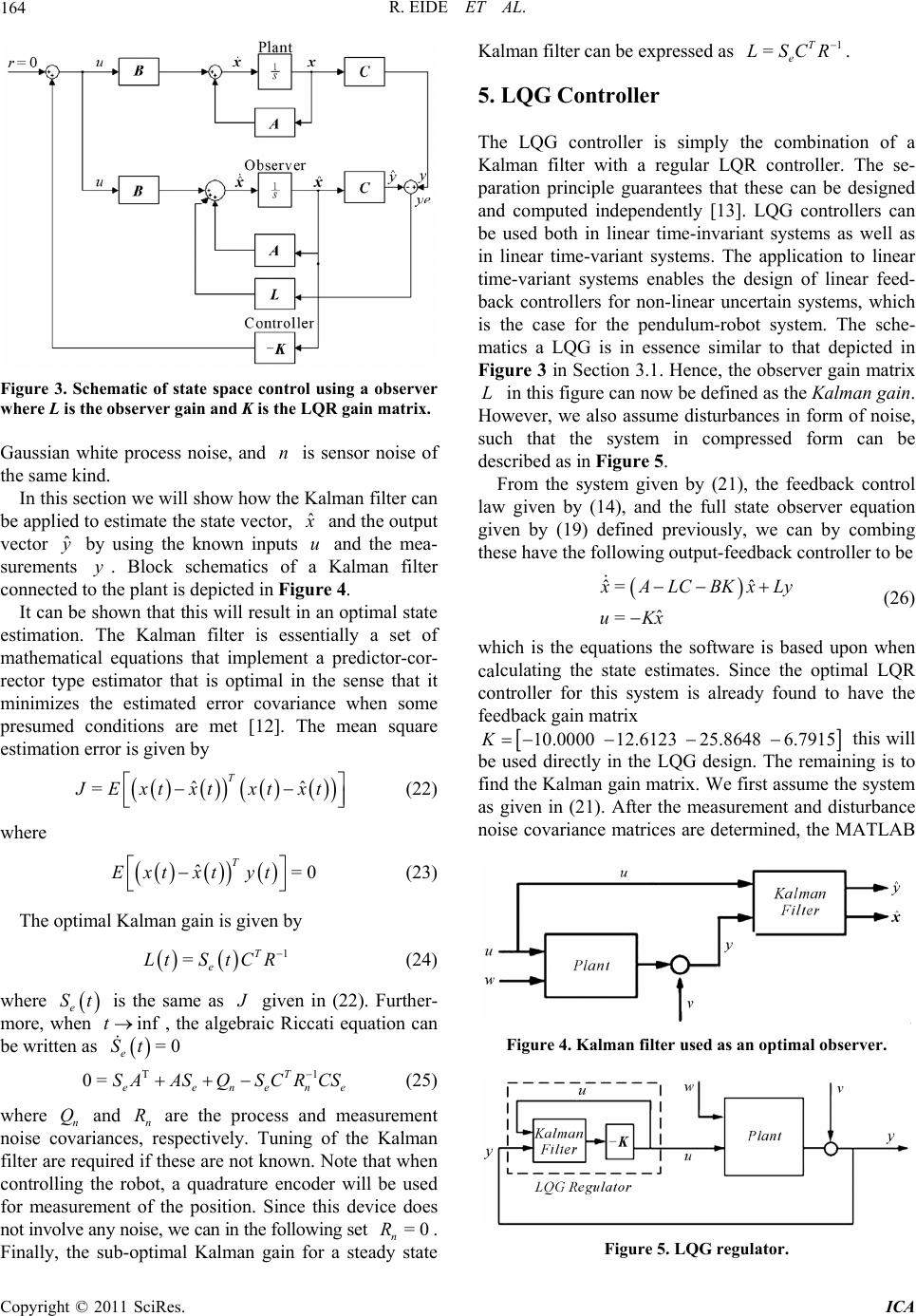

R. EIDE ET AL.

164

Figure 3. Schematic of state space control using a observer

where L is the observer gain and K is the LQR gain matrix.

Gaussian white process noise, and is sensor noise of

the same kind.

In this section we will show how the Kalman filter can

be applied to estimate the state vector,

uand the output

vector by using the known inputs and the mea-

sureme . Block schematics of a Kalman filter

connected to the plant is depicted in Figure 4.

It can be shown that this will result in an optimal state

estimation. The Kalman filter is essentially a set of

inimizes the estimated error covariance when some

is given by

nts

mathematical equations that implement a predictor-cor-

rector type estimator that is optimal in the sense that it

presumed conditions are met [12]The mean square

estimation error





 



ˆˆ



Ext xtxt xt









(22)

where







ˆ=0Ext xtyt





(23)

The optimal Kalman gain is given by

 

LtS tCR

 (24)

where



St is the same as

given in (22). Further-

more, when inft, the alge

braic Riccati equation can

be written

(25)

and are the process and measurement

noise cnpectively. Tuning

red if these are not known. Note that when

coer will be used

for me the position. Since this device does

not involv ancan in the fo

mal Kalman gain for





0= T

eenen

SAASQSCR CS





where n

ovaria

filter are requi

easurem

Finally, the sub-opti

ces, res

nt of

y noise, we

of the Kalman

ntrolling the robot, a quadrature encod

llowing set =0

a steady state

Kalman filter can be expressed as 1

LSCR



5. LQG Controller

The LQG controller is simply the combi

ar feed

ot system. The sche-

atics a LQG is in essence similar to that depicted in

nce, the observer gain matrix

in this figure can now be defined as the Kalman gain.

nation of a

Kalman filter with a regular LQR controller. The se-

paration principle guarantees that these can be designed

and computed independently [13]. LQG controllers can

be used both in linear time-invariant systems as well as

in linear time-variant systems. The application to linear

time-variant systems enables the design of line-

back controllers for non-linear uncertain systems, which

is the case for the pendulum-rob

Figure 3 in Section 3.1. He

However, we also assume disturbances in form of noise,

such that the system in compressed form can be

described as in Figure 5.

From the system given by (21), the feedback control

law given by (14), and the full state observer equation

given by (19) defined previously, we can by combing

these have the following output-feedback co ntr oller to be





ˆˆ

ALCBKxLy

uKx

 



 (26)

which is the equations the software is based upon when

lculating the state estimates. Since the optimal LQR

controller for this system is already found to have the

feedback gain matrix





10.0000 12.6123K 25.8648 6.7915 

be this will

used directly in the LQG design. The remaining is to

find the Kalman gain matrix. We first assume the system

as given in (21). After the measurement and disturbance

noise covariance matrices are determined, the MATLAB

Figure 4. Kalman filter used as an optimal observer.

Figure 5. LQG regulator.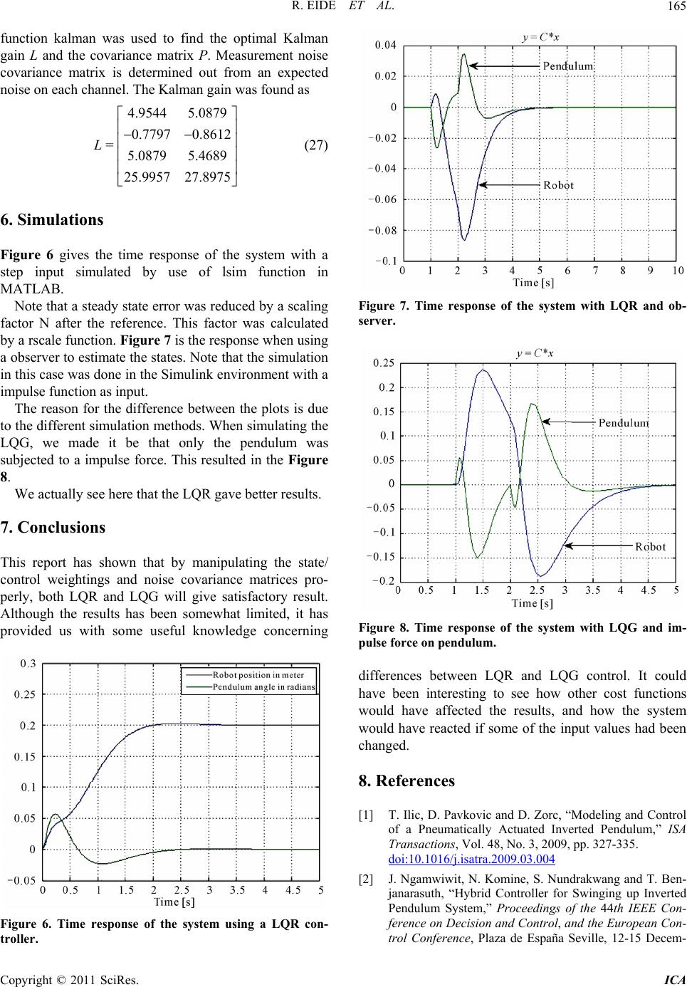

R. EIDE ET AL.165

function kalman was used to find the optimal Kalman

gain L and the covariance matrix P. Measurement noise

covariance matrix is determined out from an expected

noise on each channel. The Kalman gain was found as

(27

6. Simulations

Figure 6 gives the time response of the system with a

step input simulated by use of lsim function in

MATLAB.

Note that a steady state error was reduced by a scalin

The reason for the difference between the plots is due

to the different simulation methods. When simulating the

LQG, we made it be that only the

subjected to a impulse force. This resulted in the Figure

8. We actually see here that the LQR gave better results.

4.95445.0879

0.7797 0.8612

25.9957 27.8975











5.0879 5.4689



)

factor N after twas calculated

by a rscale function. Figure 7 is the response when u sin g

a observer to estimate the states. Note that the simulation

in this case was done in the Simulink environment with a

impulse function as input.

he reference. This factor

pendulum was

. Conclusions 7

This report has shown that by manipulating the state/

control weightings and noise covariance matrices pro-

perly, both LQR and LQG will give satisfactory result.

Although the results has been somewhat limited, it has

provided us with some useful knowledge concerning

Figure 6. Time response of the system using a LQR con-

troller.

Figure 7. Time response of the system with LQR and ob-

server.

Figure 8. Time response of the system with LQG and im-

ulse force on pendulum.

differences between LQR and LQG control. It could

have been interesting to see how other cost functions

would have affected the results, and how the system

would have reacted if some of the input values had been

changed.

8. References

[1] T. Ilic, D. Pavkovic and D. Zorc, “Modeling and Control

of a Pneumatically Actuated Inverted Pendulum,” ISA

Transactions, Vol. 48, No. 3, 2009, pp. 327-335.

doi:10.1016/j.isatra.2009.03.004

[2] J. Ngamwiwit, N. Komine, S. Nundrakwang and T. Ben-

janarasuth, “Hybrid Controller for Swinging up Inverted

Pendulum System,” Proceedings of the 44th IEEE Con-

-ference on Decision and Control, and the European Con

trol Conference, Plaza de España Seville, 12-15 Decem-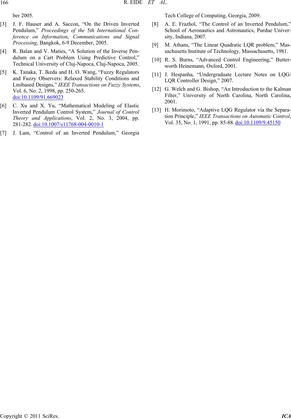

R. EIDE ET AL.

166

] J. F. Hauser and A. Saccon, “On the Driven Inverted

ical University of Cluj-Napoca, Cluj-Napoca, 2005.

Ikeda and H. O. Wang, “Fuzzy Regulators

servers: Relaxed Stability Conditions and

ber 2005.

Pendulum,” Proceedings of the 5th International Con-

ference on Information, Communications and Signal

Processing, Bangkok, 6-9 December, 2005.

[4] R. Balan and V. Maties, “A Solution of the Inverse Pen-

dulum on a Cart Problem Using Predictive Control,”

Techn

[5] K. Tanaka, T.

and Fuzzy Ob

Lmibased Designs,” IEEE Transactions on Fuzzy Systems,

Vol. 6, No. 2, 1998, pp. 250-265.

doi:10.1109/91.669023

[6] C. Xu and X. Yu, “Mathematical Modeling of Elastic

Inverted Pendulum Control System,” Journal of Control

Theory and Applications, Vol. 2, No. 3, 2004, pp.

281-282. doi:10.1007/s11768-004-0010-1

[7] J. Lam, “Control of an Inverted Pendulum,” Georgia

Tech College of Computing, Georgia, 2009.

[8] A. E. Frazhol, “The Control of an Inverted Pendulum,”

School of Aeronautics and Astronautics, Purdue Univer-

sity, Indiana, 2007.

[9] M. Athans, “The Linear Quadratic LQR problem,” Mas-

sachusetts Institute of Technology, Massachusetts, 1981.

[10] R. S. Burns, “Advanced Control Engineering,” Butter-

worth Heinemann, Oxford, 2001.

[11] J. Hespanha, “Undergraduate Lecture Notes on LQG/

LQR Controller Design,” 2007.

[12] G. Welch and G. Bishop, “An Introduction to the Kalman

Filter,” University of North Carolina, North Carolina,

2001.

[13] H. Morimoto, “Adaptive LQG Regulator via the Separa-

tion Principle,” IEEE Transactions on Automatic Control,

Vol. 35, No. 1, 1991, pp. 85-88. doi:10.1109/9.45150