Updating Geologic Models using Ensemble Kalman Filter for Water Coning Control

doi:10.4236/eng.2011.35063

Paper Menu >>

Journal Menu >>

Engineering, 2011, 3, 538-548

doi:10.4236/eng.2011.35063 Published Online May 2011 (http://www.SciRP.org/journal/eng)

Updating Geologic Models Using Ensemble Kalman Filter

for Water Coning Control

Cesar A. Mantilla, Sanjay Srinivasan, Quoc P. Nguyen

The University of Texas at Austin, Austin, USA

E-mail: [email protected]

Received February 5, 2011; revised March 15, 2011; accepted April 19, 2011

Abstract

This study investigated the feasibility of updating prior uncertain geologic models using Ensemble Kalman

filter for controlling water coning problems in horizontal wells. Current downhole data acquisition technol-

ogy allows continuous updating of the reservoir models and real-time control of well operations. Ensemble

Kalman Filter is a model updating algorithm that permits rapid assimilation of production response for res-

ervoir model updating and uncertainty assessment. The effect of the type and amount of production data on

the updated geologic models was investigated first through a synthetic reservoir model, and then imple-

mented on a laboratory experiment that simulated the production of a horizontal well affected by water con-

ing. The worth of periodic model updating for optimized production and oil recovery is demonstrated.

Keywords: Ensemble Kalman Filter, Reservoir Model Updating, Oil Production Optimization

1. Introduction

The productive life of a well completed over an active

aquifer is strongly affected by water coning. The evolu-

tion of the water cone is driven by non-uniform draw-

down pressure near the wellbore. The irreversibility of

water coning mandates its early detection, modeling and

control before and/or during water breakthrough. Recent

development in technologies for in-situ monitoring using

pressure and temperature distributed sensors allow ac-

quisition of real-time production data that carry valuable

information about reservoir properties and the water

conning process in the vicinity of the well. The acquired

data can be used to maximize oil-water ratio through

model based dynamic optimal control of pressure draw-

down along a production well and/or inflow allocation

among the wells draining the same reservoir.

Water coning is a local phenomenon governed by the

gradient of the flow potential in the vicinity of the well.

Since the flux variations in the far-field have a relatively

insignificant influence on the characteristics of coning, a

full reservoir model is not required to control this local

phenomenon. Muskat [1] presented an analytical solution

for the critical flow rate of a well in a homogeneous and

isotropic reservoir below which a stable water cone is

formed. The velocity of cone propagation is partially

determined by reservoir permeability as shown in (1).



tot c

hPlngbh P

tkDbh







 







 (1)

h is Cone height from original water-oil contact, ΔP is

the pressure difference from the tip of the cone to the

wellbore, µ is the oil viscosity, k the average permeabil-

ity, b is the distance from the well to original water-oil

contact, Δρ is the oil-water density difference, g is the

gravity force, and Pc is the capillary pressure.

Several analytical and numerical correlations that pre-

dict water coning performance accounting for more

complex geometries and heterogeneity have been devel-

oped. A comprehensive literature survey on water coning

was published by Alikhan and Ali [2]. Despite the exten-

sive work done on water coning modeling, most of the

existing models for this process are deterministic in the

sense that the reservoir properties (such as permeability k

in (1)) are assumed to be known. However, in most cases,

the knowledge of reservoir properties is limited, and un-

certainty in model parameters causes deviations in the

prediction of these physical quantities. Updating of res-

ervoir properties based on acquired dynamic data is cru-

cial. Conventional history matching techniques may not

be appropriate for this purpose since they are computa-

tionally expensive and time-consuming for real-time

integration of data. Ensemble Kalman filter has demon-

strated to be a rapid tool for subsurface process identifi-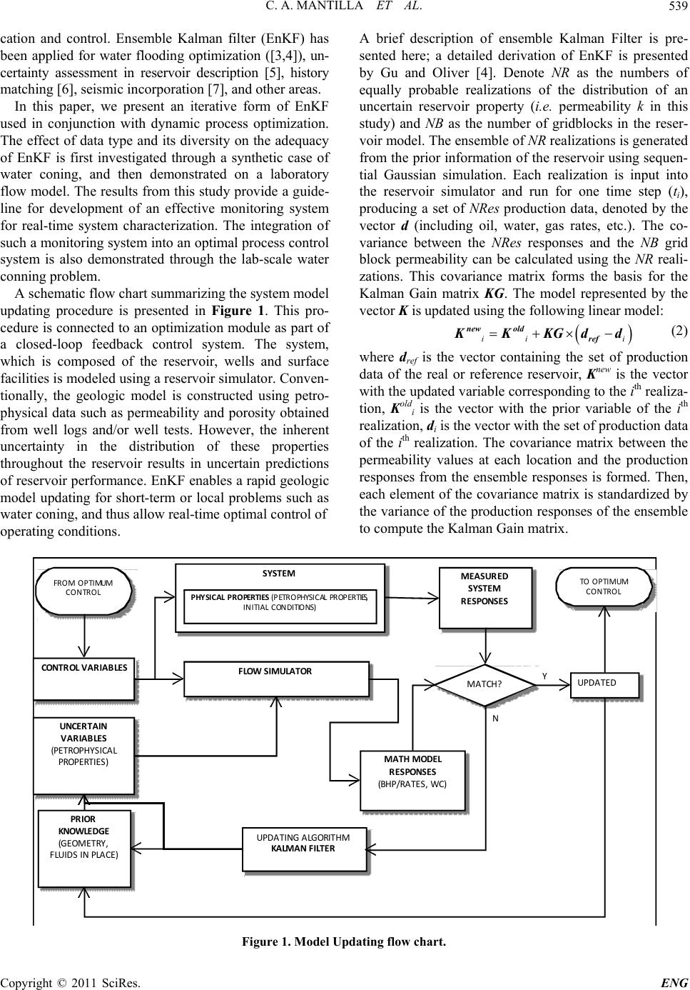

C. A. MANTILLA ET AL.539



cation and control. Ensemble Kalman filter (EnKF) has

been applied for water flooding optimization ([3,4]), un-

certainty assessment in reservoir description [5], history

matching [6], seismic incorporation [7], and other areas.

In this paper, we present an iterative form of EnKF

used in conjunction with dynamic process optimization.

The effect of data type and its diversity on the adequacy

of EnKF is first investigated through a synthetic case of

water coning, and then demonstrated on a laboratory

flow model. The results from this study provide a guide-

line for development of an effective monitoring system

for real-time system characterization. The integration of

such a monitoring system into an optimal process control

system is also demonstrated through the lab-scale water

conning problem.

A schematic flow chart summarizing the system model

updating procedure is presented in Figure 1. This pro-

cedure is connected to an optimization module as part of

a closed-loop feedback control system. The system,

which is composed of the reservoir, wells and surface

facilities is modeled using a reservoir simulator. Conven-

tionally, the geologic model is constructed using petro-

physical data such as permeability and porosity obtained

from well logs and/or well tests. However, the inherent

uncertainty in the distribution of these properties

throughout the reservoir results in uncertain predictions

of reservoir performance. EnKF enables a rapid geologic

model updating for short-term or local problems such as

water coning, and thus allow real-time optimal control of

operating conditions.

A brief description of ensemble Kalman Filter is pre-

sented here; a detailed derivation of EnKF is presented

by Gu and Oliver [4]. Denote NR as the numbers of

equally probable realizations of the distribution of an

uncertain reservoir property (i.e. permeability k in this

study) and NB as the number of gridblocks in the reser-

voir model. The ensemble of NR realizations is generated

from the prior information of the reservoir using sequen-

tial Gaussian simulation. Each realization is input into

the reservoir simulator and run for one time step (ti),

producing a set of NRes production data, denoted by the

vector d (including oil, water, gas rates, etc.). The co-

variance between the NRes responses and the NB grid

block permeability can be calculated using the NR reali-

zations. This covariance matrix forms the basis for the

Kalman Gain matrix KG. The model represented by the

vector K is updated using the following linear model:





new oldref

KKGdd

(2)

where dref is the vector containing the set of production

data of the real or reference reservoir, Knew is the vector

with the updated variable corresponding to the ith realiza-

tion, Kold

i is the vector with the prior variable of the ith

realization, di is the vector with the set of production data

of the ith realization. The covariance matrix between the

permeability values at each location and the production

responses from the ensemble responses is formed. Then,

each element of the covariance matrix is standardized by

the variance of the production responses of the ensemble

to compute the Kalman Gain matrix.

SYSTEM

CONTR OLVARIABLES

PHYSICALPR O PERTI ES(P ETROPHYSICALPR OP ER TIES,

INITIALCON DITIONS)

MEA S URE D

SYSTEM

RESPONSES

MATHMODEL

RESPONSES

(BHP/RATE S,WC)

FLOWSIMULATOR

PR IOR 

KNOWLEDGE

(GEOMETRY,

FLUIDSINPLACE )

UNCER T AIN

VARIABLES

(PETROPHYSI CAL

PROPERTIE S)

MATCH?

UPDAT ING ALGORITHM

KAL MANFILTER

YUPDATE D

FROMOPTIMUM

CON TROL

TOOPTIMUM

CONTROL

Figure 1. Model Updating flow chart.

C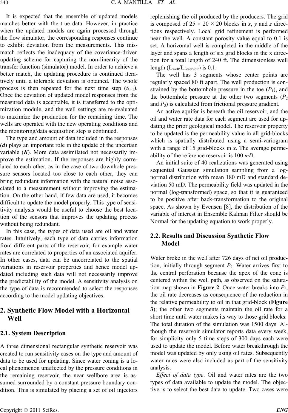. A. MANTILLA ET AL.

540

It is expected that the ensemble of updated models

matches better with the true data. However, in practice

when the updated models are again processed through

the flow simulator, the corresponding responses continue

to exhibit deviation from the measurements. This mis-

match reflects the inadequacy of the covariance-driven

updating scheme for capturing the non-linearity of the

transfer function (simulator) model. In order to achieve a

better match, the updating procedure is continued itera-

tively until a tolerable deviation is obtained. The whole

process is then repeated for the next time step (tk+1).

Once the deviation of updated model responses from the

measured data is acceptable, it is transferred to the opti-

mization module, and the well settings are re-evaluated

to maximize the production for the remaining time. The

wells are operated with the new operating conditions and

the monitoring/data acquisition step is continued.

The type and amount of data included in the responses

(d) plays an important role in the update of the uncertain

variable (K). More data assimilated not necessarily im-

prove the estimation. If the responses are highly corre-

lated to each other, as in the case of two downhole pres-

sure sensors located too close to each other, they can

bring redundant information with the natural noise asso-

ciated to a measurement without improving the estima-

tion. On the other hand, if few data are used, it becomes

difficult to update the model properly. This type of sensi-

tivity analysis would be useful to choose the best loca-

tion of the sensors that improves the updating process

without being redundant.

In this case, the types of data used are oil and water

rates. Intuitively, each type of data carries information

from different parts of the reservoir, for example water

rates are correlated to properties of an associated aquifer.

In other cases, data can be uncorrelated to the spatial

variations in reservoir properties and hence model up-

dated including such data will not necessarily improve

the predictability of the model. A sensitivity analysis on

the type of data is recommended to select the responses

according to the model updating objectives.

2. Synthetic Flow Model with a Horizontal

Well

2.1. System Description

A three dimensional rectangular synthetic reservoir was

created to run sensitivity cases on the type and amount of

data to be used for updating. Since water coning is a lo-

cal phenomenon unaffected by the pressure conditions in

the remaining reservoir, the near wellbore area is as-

sumed surrounded by a constant pressure boundary con-

dition. This is simulated by placing a set of oil injectors

replenishing the oil produced by the producers. The grid

is composed of 25 × 20 × 20 blocks in x, y and z direc-

tions respectively. Local grid refinement is performed

near the well. A constant porosity value equal to 0.1 is

set. A horizontal well is completed in the middle of the

layer and spans a length of six grid blocks in the x direc-

tion for a total length of 240 ft. The dimensionless well

length (Lwell/Lreservoir) is 0.1.

The well has 3 segments whose center points are

regularly spaced 80 ft apart. The well production is con-

strained by the bottomhole pressure in the toe (P1), and

the bottomhole pressure at the other two segments (P2

and P3) is calculated from frictional pressure gradient.

An active aquifer is beneath the oil reservoir, and the

oil and water rate data for each segment are used for up-

dating the prior geological model. The reservoir property

to be updated is the permeability value in all grid-blocks

which is spatially distributed using a semi-variogram

with a range of 15 grid-blocks in x. The average perme-

ability of the reference reservoir is 100 mD.

An initial suite of 40 realizations was generated using

sequential Gaussian simulation sampling from a log-

normal distribution with mean 180 mD and standard de-

viation 50 mD. The permeability field was updated in the

normal (log-transformed) space, so that it is guaranteed

to be positive after back-transformation to the original

space. As shown by Evensen [8], the distribution of the

variable of interest in Ensemble Kalman Filter should be

Normal for the updating equation to work properly.

2.2. Results and Discussion Synthetic Flow

Model

Water broke in the well after 726 days of net oil produc-

tion, initially through segment P2. Water arrives first to

the central perforation because the apex of the cone is

centered within the well path, as observed on the satura-

tion map shown in Figure 2. Once water breaks into P2,

the oil rate decreases as consequence of the reduction in

the relative permeability to oil in that grid-block (Figure

3); the other two segments maintain the oil rate for a

short time until water makes its way to those grid blocks.

The total duration of the simulation was 1500 days. Al-

though the reservoir simulator reports data every week,

for simplicity only 5 time steps of 300 days each were

used to update the model. Before water breakthrough the

model was updated by only using oil rates. Subsequently

water rates were also included as part of the sensitivity

analysis.

Effect of data type. Oil and water rates are the two

types of data available to update the model. The objec-

tive is to select the best data wo cases were to update. T

C. A. MANTILLA ET AL.541

Figure 2. Profile of the water cone resulting in breakthrough at 726 days.s

200

400

600

800

1000

1200

02004006008001000 1200 1400 1600

Oil Rate [m3/day]

Time (days)

Oil Rate P1

Oil Rate P2

Oil Rate P3

100

150

200

0200 400 600 800100012001400160

Water Rate [m 3/day]

Ti me ( da y s )

Water Rate P1

Water Rate P2

Water Rate P3

Figure 3. Oil production rates corresponding to the reference reservoir. Water breaks through initially in the well segment P2

and later in P1 and P3. Note that the reduction in the oil rate in P1 and P3 is less severe.

analyzed: in Case 1, water and oil rates from the 3 per-

forations were included in the objective function; and

Case 2 only the oil rate from the 3 perforations were in-

cluded, the water rate was excluded from the objective

function. Oil and water rates from each well segment

enter in the updating equation independently, and the

model is updated until each segment rate (water and oil)

satisfies the specified tolerance. In order to have a fair

comparison, the total oil and water rates from the well

(adding the three production points) are compared re-

gardless whether they are used to update the model or

not. The ultimate goal is to predict the total production of

the well, not partial rates.

Predictability. The accuracy of the updated models in

terms of the predictability of oil and water rates from

Cases 1 and 2 are compared in Figure 4. Figure 4(a)

shows the predicted oil rates for time step 3 (900 days),

at this time both cases had the same predicted oil and

water rates since in time steps 1 and 2 previous time

steps they both used only oil rates to update because wa-

ter had not breakthrough yet. After updating at 900 days,

Case 2 resulted with oil rates closer to the reference be-

cause its objective was only to reduce the mismatch the

oil rates as opposed to Case 1, where the objective was to

simultaneously reduce the mismatch in both oil and wa-

ter rates. In Case 1, the minimization of mismatch of

total (oil + water) rates causes some compromise to be

made in honoring the oil rates alone.

Although Case 2 matched closer the oil rate, the mis-

match in predicted water rate was higher than in Case 1

as shown in Figure 4(b). This is because Case 2 did not

included water rates in the updating equation. In sum-

mary, Case 2 predicts better oil rates while Case 1 pre-

dicts water rates. However, Figure 5(a) shows that the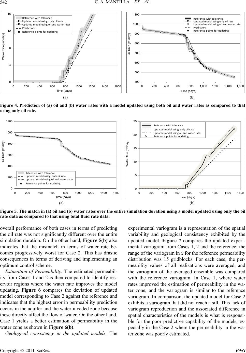

C. A. MANTILLA ET AL.

542

02004006008001000 1200 1400 1600

Water Rate [m

l/day]

Ti me ( d a y s )

Referencewithtolerance

Upda tedmodelusingonlyoilrate

Upda tedmodelusingoilandwaterrates

Predictions

Reference pointsfor updating

400

500

600

700

800

900

1000

1100

02004006008001,000 1,200 1,400 1,600

Oil Rate [m

/day]

Time (days)

Referenc ewithtolerance

Updatedmodelusingonlyoilrat e

Updatedmodelusingoilandwaterrate

Predictions

Reference pointsforupdating

(a) (b)

Figure 4. Prediction of (a) oil and (b) water rates with a model updated using both oil and water rates as compared to that

using only oil rate.

200

400

600

800

1000

1200

02004006008001000 1200 1400 1600

Oil Rate [m

/day]

Time (days)

Referencewithtolerance

Updatedmodelusingonlyoilrate

Updatedmodelusingoilandwaterrates

Reference pointsforupdating

02004006008001000 1200 1400 1600

Wat er R ate (m

/day)

Time (days)

Referencewithtolerance

Upda t ed modelusingonlyoi lrate

Upda t ed modelusingoilandwaterrates

Reference pointsforupdating

(a) (b)

Figure 5. The match in (a) oil and (b) water rates over the entire simulation duration using a model updated using only the oil

rate data as compared to that using total fluid rate data.

overall performance of both cases in terms of predicting

the oil rate was not significantly different over the entire

simulation duration. On the other hand, Figure 5(b) also

indicates that the mismatch in terms of water rate be-

comes progressively worst for Case 2. This has drastic

consequences in terms of deriving and implementing an

optimum control scheme.

Estimation of Permeability. The estimated permeabil-

ity from Cases 1 and 2 is then compared to identify res-

ervoir regions where the water rate improves the model

updating. Figure 6 compares the deviation of updated

model corresponding to Case 2 against the reference and

indicates that the highest error in permeability prediction

occurs in the aquifer and the water invaded zone because

these directly affect the flow of water. On the other hand,

Case 1 yields a better estimation of permeability in the

water zone as shown in Figure 6(b).

Geological consistency in the updated models. The

experimental variogram is a representation of the spatial

variability and geological consistency exhibited by the

updated model. Figure 7 compares the updated experi-

mental variogram from Cases 1, 2 and the reference; the

range of the variogram in x for the reference permeability

distribution was 15 gridblocks. For each case, the per-

meability values of all realizations were averaged, and

the variogram of the averaged ensemble was compared

with the reference variogram. In Case 1, where water

rates improved the estimation of permeability in the wa-

ter zone, and the variogram is similar to the reference

variogram. In comparison, the updated model for Case 2

exhibits a variogram that did not reach a sill. This lack of

variogram reproduction and the associated difference in

spatial characteristics of the models is what is responsi-

ble for the poor predictive capability of the models, es-

pecially in the Case 2 where the permeability in the wa-

ter zone was poorly estimated.

C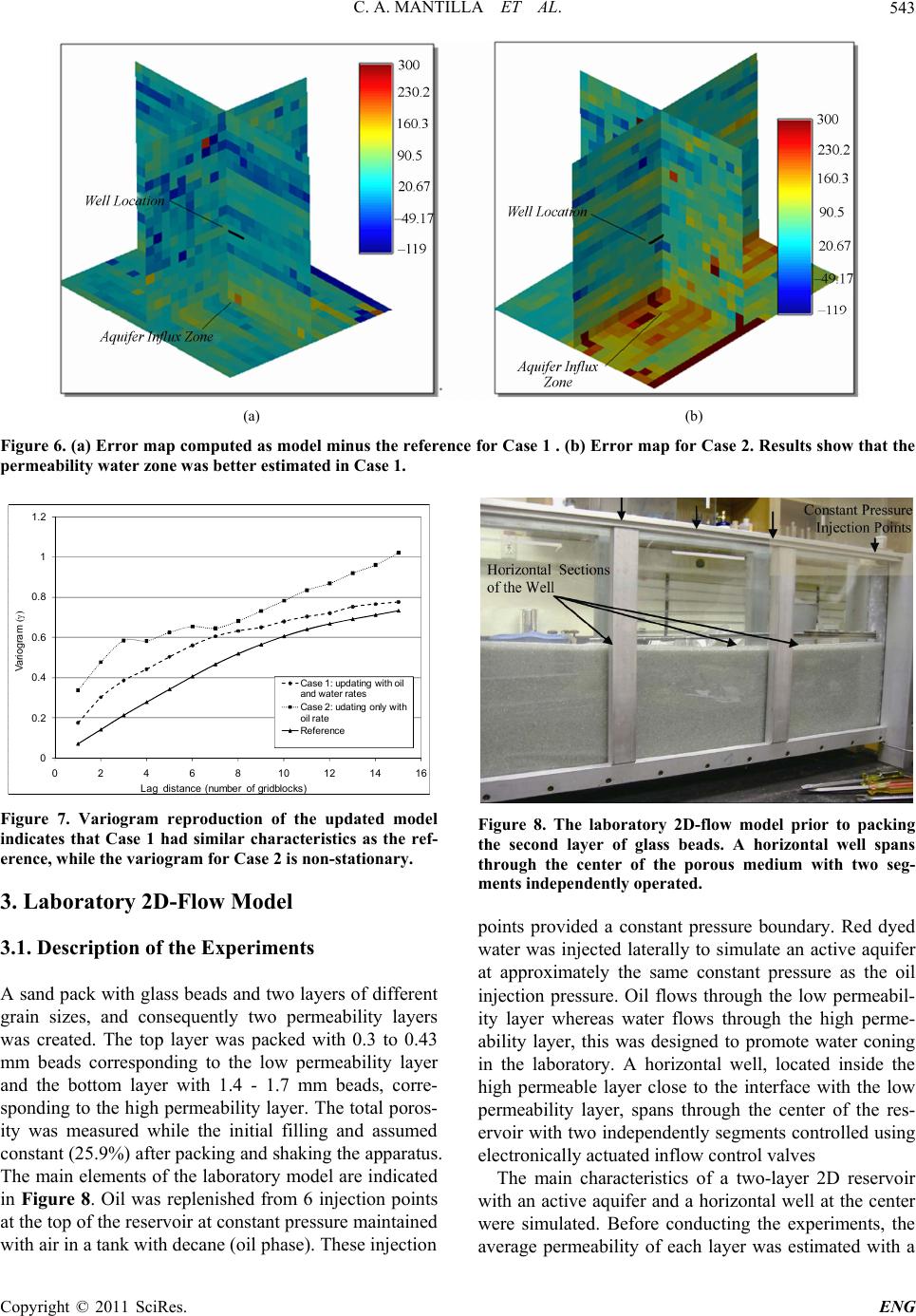. A. MANTILLA ET AL.543

(a) (b)

Figure 6. (a) Error map computed as model minus the reference for Case 1 . (b) Error map for Case 2. Results show that the

permeability water zone was better estimated in Case 1.

0.2

0.4

0.6

0.8

1.2

02468101214

Variogram 

Lag distance (number of gridblocks)

Case 1: updatin g with oil

an d water rates

Case 2: udatin g only with

oil rate

Refe r e nc e

Figure 7. Variogram reproduction of the updated model

indicates that Case 1 had similar characteristics as the ref-

erence, while the variogram for Case 2 is non-stationary.

3. Laboratory 2D-Flow Model

3.1. Description of the Experiments

A sand pack with glass beads and two layers of different

grain sizes, and consequently two permeability layers

was created. The top layer was packed with 0.3 to 0.43

mm beads corresponding to the low permeability layer

and the bottom layer with 1.4 - 1.7 mm beads, corre-

sponding to the high permeability layer. The total poros-

ity was measured while the initial filling and assumed

constant (25.9%) after packing and shaking the apparatus.

The main elements of the laboratory model are indicated

in Figure 8. Oil was replenished from 6 injection points

at the top of the reservoir at constant pressure maintained

with air in a tank with decane (oil phase). These injection

Figure 8. The laboratory 2D-flow model prior to packing

the second layer of glass beads. A horizontal well spans

through the center of the porous medium with two seg-

ments independently ope rated.

points provided a constant pressure boundary. Red dyed

water was injected laterally to simulate an active aquifer

at approximately the same constant pressure as the oil

injection pressure. Oil flows through the low permeabil-

ity layer whereas water flows through the high perme-

ability layer, this was designed to promote water coning

in the laboratory. A horizontal well, located inside the

high permeable layer close to the interface with the low

permeability layer, spans through the center of the res-

ervoir with two independently segments controlled using

electronically actuated inflow control valves

The main characteristics of a two-layer 2D reservoir

with an active aquifer and a horizontal well at the center

were simulated. Before conducting the experiments, the

average permeability of each layer was estimated with a

C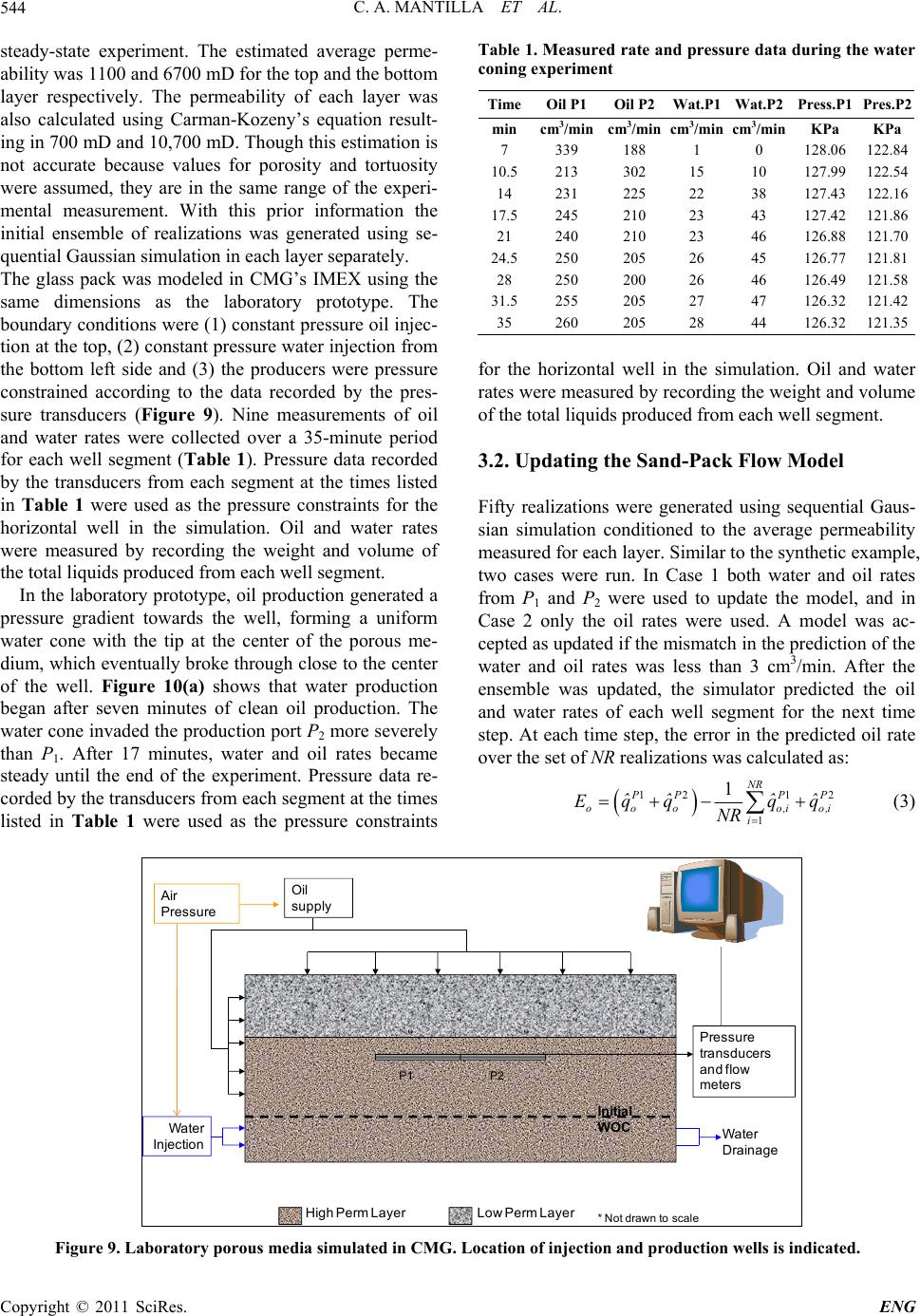. A. MANTILLA ET AL.

544

steady-state experiment. The estimated average perme-

ability was 1100 and 6700 mD for the top and the bottom

layer respectively. The permeability of each layer was

also calculated using Carman-Kozeny’s equation result-

ing in 700 mD and 10,700 mD. Though this estimation is

not accurate because values for porosity and tortuosity

were assumed, they are in the same range of the experi-

mental measurement. With this prior information the

initial ensemble of realizations was generated using se-

quential Gaussian simulation in each layer separately.

The glass pack was modeled in CMG’s IMEX using the

same dimensions as the laboratory prototype. The

boundary conditions were (1) constant pressure oil injec-

tion at the top, (2) constant pressure water injection from

the bottom left side and (3) the producers were pressure

constrained according to the data recorded by the pres-

sure transducers (Figure 9). Nine measurements of oil

and water rates were collected over a 35-minute period

for each well segment (Table 1). Pressure data recorded

by the transducers from each segment at the times listed

in Table 1 were used as the pressure constraints for the

horizontal well in the simulation. Oil and water rates

were measured by recording the weight and volume of

the total liquids produced from each well segment.

In the laboratory prototype, oil production generated a

pressure gradient towards the well, forming a uniform

water cone with the tip at the center of the porous me-

dium, which eventually broke through close to the center

of the well. Figure 10(a) shows that water production

began after seven minutes of clean oil production. The

water cone invaded the production port P2 more severely

than P1. After 17 minutes, water and oil rates became

steady until the end of the experiment. Pressure data re-

corded by the transducers from each segment at the times

listed in Table 1 were used as the pressure constraints

Table 1. Measured rate and pressure data during the water

coning experiment

TimeOil P1 Oil P2Wat.P1 Wat.P2 Press.P1Pres.P2

min cm3/min cm3/min cm3/min cm3/min KPa KPa

7 339 188 1 0 128.06122.84

10.5213 302 15 10 127.99122.54

14 231 225 22 38 127.43122.16

17.5245 210 23 43 127.42121.86

21 240 210 23 46 126.88121.70

24.5250 205 26 45 126.77121.81

28 250 200 26 46 126.49121.58

31.5255 205 27 47 126.32121.42

35 260 205 28 44 126.32121.35

for the horizontal well in the simulation. Oil and water

rates were measured by recording the weight and volume

of the total liquids produced from each well segment.

3.2. Updating the Sand-Pack Flow Model

Fifty realizations were generated using sequential Gaus-

sian simulation conditioned to the average permeability

measured for each layer. Similar to the synthetic example,

two cases were run. In Case 1 both water and oil rates

from P1 and P2 were used to update the model, and in

Case 2 only the oil rates were used. A model was ac-

cepted as updated if the mismatch in the prediction of the

water and oil rates was less than 3 cm3/min. After the

ensemble was updated, the simulator predicted the oil

and water rates of each well segment for the next time

step. At each time step, the error in the predicted oil rate

over the set of NR realizations was calculated as:



12 1

1NR 2

ooo o,io

ˆˆ ˆˆ

Eqq qq

NR 

 

P

(3)

Water

Drainage

High Perm LayerLow Perm Layer

Initial

WOC

Water

In je c tio n

Oil

supply

Air

Pressure

P1 P2

Pressure

transducers

and flow

meters

* Not dr awn t o scale

Figure 9. Laboratory porous media simulated in CMG. Loc ation of injection and production wells is indicated.

C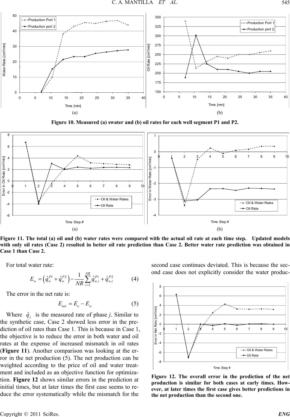. A. MANTILLA ET AL.545

0510 15 20 25 30 35 40

Water Rate [cm

/min]

Time

[

min

]

Production Port 1

Pr o duc t i o n po r t 2

150

175

200

225

250

275

300

325

350

0510 15 20 25 30 35 40

Oil Rate [cm

/min]

Ti me [ m i n]

Pr o duc t i on Po r t 1

Pr o duc t i on po rt 2

(a) (b)

Figure 10. Measured (a) swater and (b) oil rates for each well segment P1 and P2.

-6

-4

-2

012345678910

Error in Oil Rate [cm

/min]

Ti me S t e

Oil & Water Rates

Oil Rate

-4

-3

-2

-1

0123456789

Error in Water Rate [cm

/min]

Ti me S t e p #

Oil & Water Rates

Oil Rate

(a) (b)

Figure 11. The total (a) oil and (b) water rates were compared with the actual oil rate at each time step. Updated models

with only oil rates (Case 2) resulted in better oil rate prediction than Case 2. Better water rate prediction was obtained in

Case 1 than Case 2.

For total water rate:



12 1

1NR 2

www w,iw

ˆˆ ˆˆ

Eqq qq

NR 

 

P

(4)

The error in the net rate is:

neto w

EEE (5)

Where

q is the measured rate of phase j. Similar to

the synthetic case, Case 2 showed less error in the pre-

diction of oil rates than Case 1. This is because in Case 1,

the objective is to reduce the error in both water and oil

rates at the expense of increased mismatch in oil rates

(Figure 11). Another comparison was looking at the er-

ror in the net production (5). The net production can be

weighted according to the price of oil and water treat-

ment and included as an objective function for optimiza-

tion. Figure 12 shows similar errors in the prediction at

initial times, but at later times the first case seems to re-

duce the error systematically while the mismatch for the

second case continues deviated. This is because the sec-

ond case does not explicitly consider the water produc-

-8

-6

-4

-2

0123456789

Error in Net Rate [cm

/min]

Ti me S te

Oil & Water Rates

Oil Rate

Figure 12. The overall error in the prediction of the net

production is similar for both cases at early times. How-

ever, at later times the first case gives better predictions in

the net production than the se cond one.

C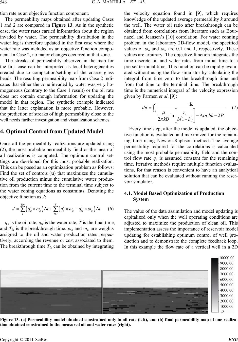. A. MANTILLA ET AL.

546

tion rate as an objective function component.

The permeability maps obtained after updating Cases

1 and 2 are compared in Figure 13. As in the synthetic

case, the water rates carried information about the region

invaded by water. The permeability distribution in the

water leg is therefore updated in the first case where the

water rate was included as an objective function compo-

nent. In Case 2, no major changes occurred in that zone.

The streaks of permeability observed in the map for

the first case can be interpreted as local heterogeneities

created due to compaction/settling of the coarse glass

beads. The resulting permeability map from Case 2 indi-

cates that either the zone invaded by water was very ho-

mogeneous (contrary to the Case 1 result) or the oil rate

does not contain enough information for updating the

model in that region. The synthetic example indicated

that the latter explanation is more probable. However,

the prediction of streaks of high permeability close to the

well needs further investigation and visualization schemes.

4. Optimal Control from Updated Model

Once all the permeability realizations are updated using

(2), the most probable permeability field or the mean of

all realizations is computed. The optimum control set-

tings are developed for this most probable realization.

This can be posed as an optimization problem as follows:

Find the set of controls (u) that maximizes the cumula-

tive oil production minus the cumulative water produc-

tion from the current time to the terminal time subject to

the water coning equations as constraints. Denoting the

objective function as J:

 

Tbt T

ttt

oo ooww

tTbt

qtqq





 t



 (6)

qo is the oil rate, qw is the water rate, T is the final time,

and Tbt is the breakthrough time. ωo and ωw are weights

assigned to the oil and water production rates respec-

tively, according the revenue or cost associated to them.

The breakthrough time Tbt can be obtained by integrating

the velocity equation found in [9], which requires

knowledge of the updated average permeability k around

the well. The water oil ratio after breakthrough can be

obtained from correlations from literature such as Bour-

nazel and Jeansen’s [10] correlation. For water conning

problem in the laboratory 2D-flow model, the specified

values of ωo and ωw are 0.1 and 1, respectively. These

values are arbitrary. The objective function integrates the

time discrete oil and water rates from initial time to a

pre-set terminal time. This function can be rapidly evalu-

ated without using the flow simulator by calculating the

integral from time zero to the breakthrough time and

from that time to the terminal time. The breakthrough

time is the numerical integral of the velocity expression

given by Farmen et al. [9]:



ln 2

tbt

bh P

kD bh







 







 (7)

Every time step, after the model is updated, the objec-

tive function is evaluated and maximized for the remain-

ing time using Newton-Raphson method. The average

permeability required for the correlations is calculated

using the most probable permeability field and the con-

trol flow rate qo is assumed constant for the remaining

time. Iterative methods require multiple function evalua-

tions, for that reason is convenient to have an analytical

solution that can be evaluated without running the reser-

voir simulator.

4.1. Model Based Optimization of Production

System

The value of the data assimilation and model updating is

capitalized only when the well operating conditions are

adjusted to maximize the production of clean oil. This

implementation assess the importance of reservoir model

updating for establishing optimum control of well pro-

duction and to demonstrate the complete feedback loop.

In this example the flow rate of a vertical well in a 2D

Figure 13. (a) Permeability model obtained constrained only to oil rate (left), and (b) final permeability map of one realiza-

tion obtained constrained to the measured oil and water rates (right).

C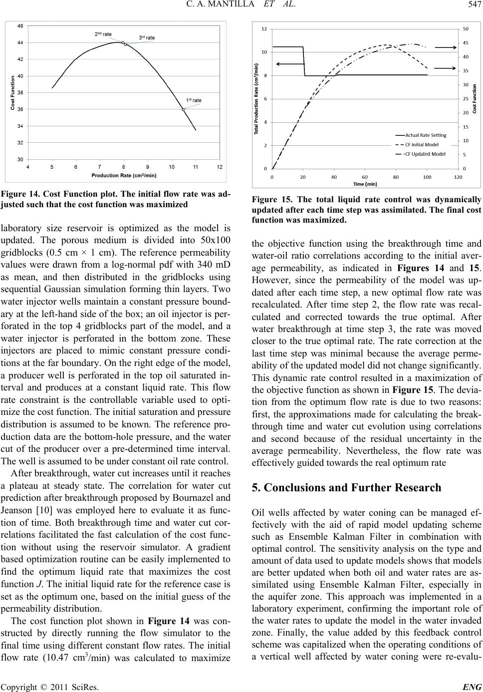. A. MANTILLA ET AL.

547

Figure 14. Cost Function plot. The initial flow rate was ad-

justed such that the cost function was maximized

laboratory size reservoir is optimized as the model is

updated. The porous medium is divided into 50x100

gridblocks (0.5 cm × 1 cm). The reference permeability

values were drawn from a log-normal pdf with 340 mD

as mean, and then distributed in the gridblocks using

sequential Gaussian simulation forming thin layers. Two

water injector wells maintain a constant pressure bound-

ary at the left-hand side of the box; an oil injector is per-

forated in the top 4 gridblocks part of the model, and a

water injector is perforated in the bottom zone. These

injectors are placed to mimic constant pressure condi-

tions at the far boundary. On the right edge of the model,

a producer well is perforated in the top oil saturated in-

terval and produces at a constant liquid rate. This flow

rate constraint is the controllable variable used to opti-

mize the cost function. The initial saturation and pressure

distribution is assumed to be known. The reference pro-

duction data are the bottom-hole pressure, and the water

cut of the producer over a pre-determined time interval.

The well is assumed to be under constant oil rate control.

After breakthrough, water cut increases until it reaches

a plateau at steady state. The correlation for water cut

prediction after breakthrough proposed by Bournazel and

Jeanson [10] was employed here to evaluate it as func-

tion of time. Both breakthrough time and water cut cor-

relations facilitated the fast calculation of the cost func-

tion without using the reservoir simulator. A gradient

based optimization routine can be easily implemented to

find the optimum liquid rate that maximizes the cost

function J. The initial liquid rate for the reference case is

set as the optimum one, based on the initial guess of the

permeability distribution.

The cost function plot shown in Figure 14 was con-

structed by directly running the flow simulator to the

final time using different constant flow rates. The initial

flow rate (10.47 cm3/min) was calculated to maximize

Figure 15. The total liquid rate control was dynamically

updated after each time step was assimilated. The final cost

function was maximized.

the objective function using the breakthrough time and

water-oil ratio correlations according to the initial aver-

age permeability, as indicated in Figures 14 and 15.

However, since the permeability of the model was up-

dated after each time step, a new optimal flow rate was

recalculated. After time step 2, the flow rate was recal-

culated and corrected towards the true optimal. After

water breakthrough at time step 3, the rate was moved

closer to the true optimal rate. The rate correction at the

last time step was minimal because the average perme-

ability of the updated model did not change significantly.

This dynamic rate control resulted in a maximization of

the objective function as shown in Figure 15. The devia-

tion from the optimum flow rate is due to two reasons:

first, the approximations made for calculating the break-

through time and water cut evolution using correlations

and second because of the residual uncertainty in the

average permeability. Nevertheless, the flow rate was

effectively guided towards the real optimum rate

5. Conclusions and Further Research

Oil wells affected by water coning can be managed ef-

fectively with the aid of rapid model updating scheme

such as Ensemble Kalman Filter in combination with

optimal control. The sensitivity analysis on the type and

amount of data used to update models shows that models

are better updated when both oil and water rates are as-

similated using Ensemble Kalman Filter, especially in

the aquifer zone. This approach was implemented in a

laboratory experiment, confirming the important role of

the water rates to update the model in the water invaded

zone. Finally, the value added by this feedback control

scheme was capitalized when the operating conditions of

a vertical well affected by water coning were re-evalu-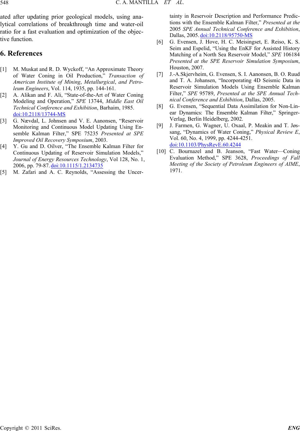

C. A. MANTILLA ET AL.

548

ated after updating prior geological models, using ana-

lytical correlations of breakthrough time and water-oil

ratio for a fast evaluation and optimization of the objec-

tive function.

6. References

[1] M. Muskat and R. D. Wyckoff, “An Approximate Theory

of Water Coning in Oil Production,” Transaction of

American Institute of Mining, Metallurgical, and Petro-

leum Engineers, Vol. 114, 1935, pp. 144-161.

[2] A. Alikan and F. Ali, “State-of-the-Art of Water Coning

Modeling and Operation,” SPE 13744, Middle East Oil

Technical Conference and Exhibition, Barhaim, 1985.

doi:10.2118/13744-MS

[3] G. Nævdal, L. Johnsen and V. E. Aanonsen, “Reservoir

Monitoring and Continuous Model Updating Using En-

semble Kalman Filter,” SPE 75235 Presented at SPE

Improved Oil Recovery Symposium, 2003.

[4] Y. Gu and D. Oilver, “The Ensemble Kalman Filter for

Continuous Updating of Reservoir Simulation Models,”

Journal of Energy Resources Technology, Vol 128, No. 1,

2006, pp. 79-87. doi:10.1115/1.2134735

[5] M. Zafari and A. C. Reynolds, “Assessing the Uncer-

tainty in Reservoir Description and Performance Predic-

tions with the Ensemble Kalman Filter,” Presented at the

2005 SPE Annual Technical Conference and Exhibition,

Dallas, 2005. doi:10.2118/95750-MS

[6] G. Evensen, J. Hove, H. C. Meisingset, E. Reiso, K. S.

Seim and Espelid, “Using the EnKF for Assisted History

Matching of a North Sea Reservoir Model,” SPE 106184

Presented at the SPE Reservoir Simulation Symposium,

Houston, 2007.

[7] J.-A.Skjervheim, G. Evensen, S. I. Aanonsen, B. O. Ruud

and T. A. Johansen, “Incorporating 4D Seismic Data in

Reservoir Simulation Models Using Ensemble Kalman

Filter,” SPE 95789, Presented at the SPE Annual Tech-

nical Conference and Exhibition, Dallas, 2005.

[8] G. Evensen, “Sequential Data Assimilation for Non-Lin-

ear Dynamics: The Ensemble Kalman Filter,” Springer-

Verlag, Berlin Heidelberg, 2002.

[9] J. Farmen, G. Wagner, U. Oxaal, P. Meakin and T. Jøs-

sang, “Dynamics of Water Coning,” Physical Review E,

Vol. 60, No. 4, 1999, pp. 4244-4251.

doi:10.1103/PhysRevE.60.4244

[10] C. Bournazel and B. Jeanson, “Fast Water—Coning

Evaluation Method,” SPE 3628, Proceedings of Fall

Meeting of the Society of Petroleum Engineers of AIME,

1971.