

Paper Menu >>
Journal Menu >>
 The Third Kind Of Particles ShaoXu Ren Institute of physical science and Engineering Tongji University, 200092, Shanghai, China Corresponding email:[email protected] ABSTRACT There are two kinds of spin particles in nature, the Bosonand the Fermion. Those with integer value spin 0,1,2...are called Bosons, with half-integer value spin /2, 3/2, 5/2...are called Fermions. It is well known that everything in the universe is made of Bosons and Fermions. The spin representations of Boson and the Fermion in conventional quantum mechanics are expressed by Hermitian matrices, whichare finite dimensional matrices. Are there so-called the Third Kind Of Particles (TKP), for an example,whose spin maybe /3, /4, /5,/6..., which are neither Bosons nor Fermions? This article concerns about the possible math figure of TKP. More detailed material related to derivative process and ideasevolvement of TKP are given. keywords The Third Kind Of Particles TKP; Boson; Fermion; Hermitian matrices; non-Hermitian matrices;Hermitian self-adjoint; positive definite non-Hermitian self-adjoint; finite dimensional matrices; infinite dimensional matrices Introduction All physical observables of conventional quantum mechanicsare Hermitian operators. These Hermitian operators Zare defined in Euclidian Space. They satisfy the so-called Hermiticity relation ZZand havereal eigenvalues. But we know that some non-Hermitian operators could also have real eigenvalues; some operators possessingreal eigenvalues might be non-Hermitian operators. TheHermiticity of an operator is only a sufficient condition, which guarantees real eigenvalues, it is not a necessary condition. In recent years, much intensive research efforts have been madeinthefieldof non-Hermitian Hamiltonians with real eigenvalues byPHHQP cite: [1],International Workshop on Pseudo-Hermitian Hamiltoniansin Quantum Physics This paper focuses on the topic of the construction of non-Hermitian angular momentum: 1) Non-Hermitian orbital angular momentum operatorLjare given, we find the eigenvalues of non-Hermitian orbital angular operator L3can be nonintegral and the wavefunctions of L3still remain to be single-values 2) Non-Hermitian spin angular momentumoperator j,n (j1, 2, 3)aregiven,we find the eigenvalue nof non-Hermitian spin operator j,n can be those of neither Bosons nor Fermions, such kind of spin particles are called The Third Kind Of Particles,TKP.TKP exist in three system,which are not Anyons. JournalofModernPhysics,2014,5,800‐869 PublishedOnlineJune2014inSciRes.http://www.scirp.org/journal/jmp http://dx.doi.org/10.4236/jmp.2014.59090 Howtocitethispaper:Ren,S.X.(2014)TheThirdKindofParticles.JournalofModernPhysics,5,800‐869. http://dx.doi.org/10.4236/jmp.2014.59090  0WhyDoesconventional spin angular momentum only...... Conventional Spin Angular Momentum Only Possess Eigenvalues with Integer and Half-integer ? a) Using commutation(1) that between angular momentum operator J2and operator J3 J2,J3−0 (1) and two eigen-equations (2),(3) J2|,|,,≥0 J3|,|,,2≥0 (2) (3) obtain J2−J3 2|,−2|, (4) b) As J2J3 2J1 2J2 2,another eigen-equation (5) is given as J1 2J2 2|,J2−J3 2|,−2|, (5) Due to J1 2J2 2is positive Hermitianoperator, (5) implies −2≧0 or 2≦ (6) (7) (7) meansSo 2,oris restricted by ! or by following two recurrence conditions (12),(15) or by following two formulas (14),(17) or by being restricted under conditions (21),(22) (8) (9) (10) (11) c) Further, there exist a top state|,maxsuch that it can’t be raised,suppose max.that is J|,max0 (12) then J−J|,max0 J2−J3 2−J3|,max0 −max 2−max|,max0 (13) (13) showing that max 2max ★ (14)  d) Similar processing, there exist abottomstate|,minsuch that it can’t be lowered,suppose min.that is J−|,min0 (15) then JJ−|,min0 J2−J3 2J3|,min0 −min 2min|,min0 (16) (16) showing that min 2−min ♣ (17) e) From ★(14) and ♣, (17),get max 2max min 2−min (18) obtain min −max (19) f) There are kstates between |,minand |,max kmax −minmax −−max2max (20) hence the maximumvalue of angular momentunofparticle is max k/2 where k0, 1, 2, 3. . . (21) (22) Two important expressions(23) and (24) are given,see below: g) Substituting (21) into (14), obtain the eigenvalue (23) of J2 max 2max ★maxmax 1k/2 k/2 1 (23) h) The dimensional formula Dof angular momentum isgiven by (24) , D2max 1k1 (24) Formula (24) is suitable for both orbit and spin. i) For orbital angular momentum, its eigenvalue state |,(3) leads take k0,2,4,6,... eigenvalue of orbitalmax k/2 0,1,2,3,... integer dimensionality of functionD2max 11, 3, 5, 7. . . (25.1) (25.2) (25.3) j) For spin angular momentum, itseigenvalue state |,(3),there are two choices of k.leads two kinds of spin particle asbelow The First Kind of Particles : Boson Particles: take k0,2,4,6,... eigenvalues of spinmax k/2 0,1,2,3,... integer dimensionality of matrixD2max 11, 3, 5, 7. . . (26.1) (26.2) (26.3) The Second Kind of Particles : FermionParticles: take k1,3,5,7,... eigenvalues of spinmax k/2 1/2,3/2,5/2,7/2,... half-integer dimensionality of matrixD2max 12,4,6,8,... (27.1) (27.2) (27.3) 0What Will HappenIf Condition (6) Is Broken ? If Condition (6) Is Broken ? A)Obviously if: the restriction (6) or equivalent to (9) or (12), (15) on operation J|,and operation J−|,are removed, then there will appearinfinite eigenvectors |,jof J3: J3|,jj|,j or jmax jmin − (28) (29.1) (29.2) B)Specially further if: the restriction (6) or (7) is broken, and is changed into the restriction (30) or (31) −20 or 2 (30) (31) (30) implies: eigenvalues (5) of J1 2J2 2should be less than zero, that is J1 2J2 2|,−2|,( negative eigenvalues)|, (32) (32) shows: J1 2J2 2is no long a positive definite operator Hence J1is non-Hermitian operator! J2is non-Hermitian operator! (33) (34.1) (34.2) C)Formula (34) is one of author’s motivation for being engrossed in Non-Hermitian angular momentum and TKP.  0The Flow of This Paper Consists of Three Parts: Part 1 0Why does ......? ;What Will happen If ..... 1Non-Hermitian Spin Angular Momentum T 2Non-Hermitian Orbital Angular MomentumL 3Eigenvalues and Eigenvalues Functions of L3 4TheRecurrence Formulaeof NormalizedWavefunctions m,n:CmEm,n Part 2 5Semi-Infinite Dimensional Matrices j,n :SpinHierarchy SH 6Infinite Dimensional Representationsj,n :ChaosSpinHierarchy CSH 7Spin 0CSH 0, 0, ,j,0 8Spin /2 CSH 3/4, 1/2, ,j,1/2 9Spin /3 CSH 4/9, 1/3, ,Δj,1/3 Part 3 10 Non-Hermitian Momentum P,Phase Factor of FractionalStatistics 11 Conclusion Appendix :Infinitesimal Rotation of TKP In chapter 0,After reviewing the math picture of angular momentumin conventional quantum mechanics, author postlates the key to TKP is to define the construction of non-Hermitian angular momentum operatorsand to extend the dimensionality of matrix representationsof those operators to semi-infinite dimensional, infinite dimensional space. The possible math figure of TKP J1and J2should be infinite (semi-infinite) dimensional non-Hermitian matrices(35) J2and J3are infinite (semi-infinite) dimensional Hermitian diagonal matrices(36) Chapter 1introduces non-Hermitiantwo dimensions spinor matrices T,which contain one space variable .In space h,Tare good spin operators. 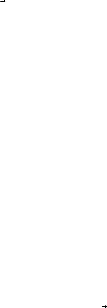 In chapter 2,Tare applied to construct non-Hermitian orbital angular momentumoperator Ljin space hg. Chapter 3shows that L3can present nonintegral eigenvalues and the wavefunctions of L3still remain to be single-values. In chapter 4,it is marvellously revealed that therecurrence formulae obtained from rising operator Land lowering operatorL−, arenobounded. The substance from chapter 2to chapter4are related to space coordinates. And the mathematical underpinningsof the next five chapters, chapter5to chapter 9, are tightly relevent to matrices whose math elements are pure complex numbers. Chapter 5introduces notions, ket vector |m,nand bra vector〈m,n|| ≡〈m,n| with m0,1,2,3...,to construct the bases of linear space,in which semi-infinite dimensional matrix representations j,n of orbital angular momentum Ljof TKP are given.j,n are called Spin Hierarchy(SH) Chapter 6extends the range of quantumnumber mto be m0, 1, 2, 3..., then infinite dimensional matrix representations,j,n are obtained. j,n are called Chaos Spin Hierarchy (CSH) The values of quantum number mquoted in chapter 5and chapter 6is ranging between 0 and ,as expected inchapter 0. In order to illustrate the character of CSH,three typical spin particles are analysed in Chapter7,8,9. Chapter 7is Boson case j,0of CSH, where quantumnumber nn00. j,0named Island Operator, hasthree diagonal blocks in its matrix representations. Chapter 8is Fermion case j,1/2 ofCSH, where quantum number nn1/2 1/2. j,1/2 named IslandOperator, has three diagonal blocks in its matrix representations. In chapter 9,quantum number nis taken to be the greatest non-integer and non-half-integer, n1/3 1/3.Use symbolΔj,1/3,named Ocean Operator, for CSH matrix representations, that has two diagonal blocks. Chapter 10 studies non-Hermitian momentum P, investigates a specialpractical applications of gauge invariance in space frgh. It is argued that the phenomenon of phase factor of fractional statistics could be explained by the concept of TKP which are more physical realistic than Anyonsare. 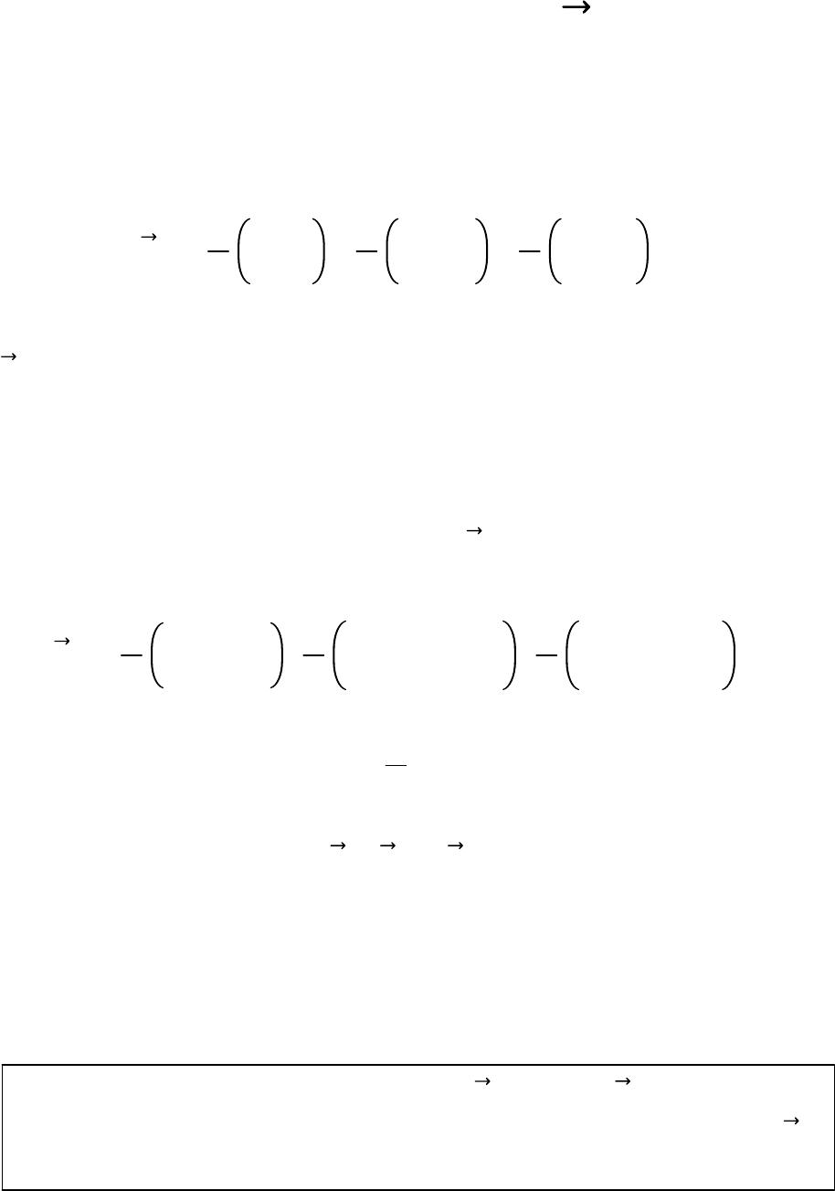 1Non-Hermitian Spin Angular Momentum T We startfrom an example of /2 spin angular momentum, its spinrepresentation (1) is the well known 22 dimensional matrix. Its three components S1,S2,S3are all Hermitianmatrices (2)and their eigenvalues are all/2. S1 2 01 10 ,1 2 0−i i0,1 2 10 0−1 (1) S1 S1,S2 S2,S3 S3 (2) Ssatisfies commutation relations SjSk−SkSjiSl (3) j,k,l1,2,3 are circulative. For convenience, sometimes we choose 1. 1.1 Non-Hermitian Spin Angular Momentum T Now introduce a set of new operators as following T1 2 0e−i ei0,1 2 −i−ie−i ieii,1 2 e−i −ei− (4) where ,are real numbersand T1 2T2 2T3 21 4,2−21 (5) T1,T2,T3obey commutation relation TTiT (6) Obviously T1is a Hermitian matrix, but T2and T3are non-Hermitian matrices. T1 T1,T2 ≠T2,T3 ≠T3 (7) but the eigenvalues of T1,T2,T3are still real numbers 1/2. Note when approaches to zero,T(4) back toS(2) In the following paragraphs, it is shown that the math defect (7) of T could be corrected from researching the inner product space of spin operator. 1.2 Hermitian Self-Adjoint Representation of Operator Z: Hermitian Operator ZZ Frist,we define the inner product space f,g≡df∗gg,f∗ (8) superscript sign ∗is complex conjugatioin. (8) represents integral for continuous variable, and represents matrix scalar multiplication for discontinuous variable.f and gare the vector functions in inner product space. Then,adjoint operation representation of an operator Zin inner product space (8) can be defined as the operator Zsuch that g,Zf≡f,Zg∗Zg,f (9) Where g,Zf≡f,Zg∗Z≡Z∗~ f,Zg∗Zg,ff,gg,f∗ (9.1) (9.2) ~ denotes transpose of a matrix Z.If the right side of (9) satisfies Zg,fg,Zf (10) then (9) becomes g,Zf≡f,Zg∗Zg,fg,Zf (11) we get operator relation ZZ (12) In case of (12), operator Zis said to be "Hermitian self-adjoint", or to be "self-adjoint" or "Hermitian". Asyet all the operators of conventional quantum mechanics are postulated to be Hermitian operators. Sometimes, space (8) is called Hermitian Space. OperatorZsatisfying formula (9) is saidto be "positive definite operator" in inner product space (8). 1.3Positive definitenon-Hermitian Self-AdjointRepresentation of OperatorZ: Non-Hermitian self-adjoint Operator Z⊕Z Extending the definition (8) of the inner product space to space (13) f,g≡df∗gg,f∗ (13) Here is a metric coefficient operator.,is introducedto be the sign of the curve of space.when →1,(13) →(8), space is flat. Hermitian Space(10) is flat space;when≠1,space becomesbent and warped. Positive Definite Non-Hermitian adjoint operation of an operator Zin inner product space (13) is defined by operator Z⊕,"⊕"called circled dag, suchthat g,Z⊕ff,Zg∗ (14) If Z⊕Z (15) then the Zis said to be "Positive Definite Non-Hermitian self-adjoint Operator". incaseof(15),cite: [2] Next we are going to seek for the explicit expressions of Z⊕,inthe case of Z that are derivative operator (A) and matrix operator(B).  A) Firstly, turn to the definition (14) of adjoint representation ∂x ⊕of a derivative operator ∂x≡∂ ∂x,we have dxg∗∂x ⊕fdxf∗∂xg∗ (16) We know what is ∂x,but not know what ∂x ⊕means, we want to find out the explicit expression of operator ∂x ⊕in the left side of (16). From theright side of(16), (F≡f), we have dxf∗∂xg∗dxf∂xg∗dxF∂xg∗Fg∗|a b−dx∂xFg∗ 0−dx∂xFg∗−dx∂xfg∗−dxg∗∂xf −dxg∗∂xf∂xf−dxg∗∂x∂xf (17) Fromtheleftsideof(16),wehave dxg∗∂x ⊕fdx∗g∗∂x ⊕fdxg∗∗~∂x ⊕f dxg∗∂x ⊕fdxg∗∂x ⊕f (18) Comparing formula (18) withformula (17),we deducethat dxg∗∂x ⊕f−dxg∗∂x∂xf (19) further ∂x ⊕−∂x−∂x ∂x ⊕−∂x−−1∂x (20) (21) and −i∂x⊕−i∂x−i−1∂x −i∂x−i1 2−1∂x⊕−i∂x−i1 2−1∂x (22) (23) B) Secondly, turn to the definition (14) of adjoint representation Z⊕of a matrix operator Zin inner product space f,g.Postulating 12 34 ,,Det 1 (24) then base on g,Z⊕ff,Zg∗(14), following we can find the explicit expression of matrix operator Z⊕: 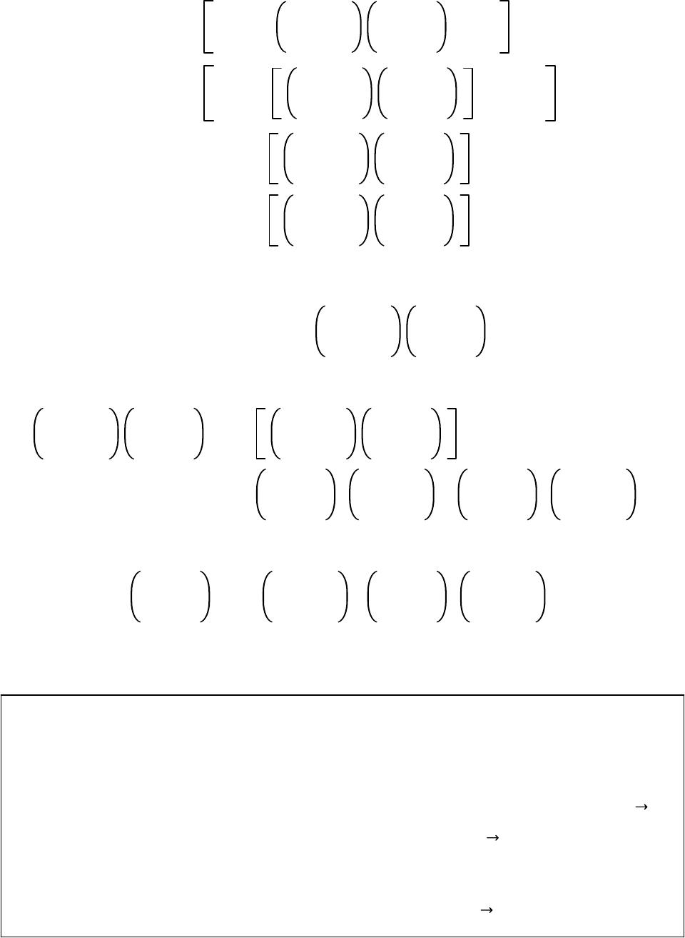 From theright side of (14), we have f,Zg∗f1,f2∗12 34 z1z2 z3z4 g1 g2 ∗ (g1,g2)12 34 z1z2 z3z4 ~ f1 f2 ∗ ∗ g1,g2∗12 34 z1z2 z3z4 ~∗ f1 f2 g1,g2∗12 34 z1z2 z3z4 f1 f2 (25) Fromtheleftsideof(14),wehave g,Z⊕fg1g2∗12 34 z1z2 z3z4 ⊕ f1 f2 (26) Comparing formula (26) withformula (25), we deduce that 12 34 z1z2 z3z4 ⊕ 12 34 z1z2 z3z4 z1z2 z3z4 12 34 z1z2 z3z4 12 34 (27) Further obtain z1z2 z3z4 ⊕ 12 34 −1z1z2 z3z4 12 34 (28) or Z⊕−1Z (29) Note Positive definite non-Hermitian Self-Adjoint Representation Z⊕ofOperator Z when Zis derivative operator Z∂x, then∂x ⊕−∂x−−1∂x(21) will be used in constructing non-Hermitian ortital angular momentumoperator L and non-Hermitian momentum operator P when Zis matrix operator,thenZ⊕−1Z(29) will be used in constructing non-Hermitianspin operator T,just see next...... 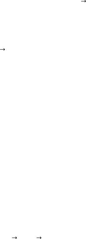 1.4 Non-Hermitian Spin Angular Momentum Operator TIs a Good Operator Again pay more attention to the fact: T1 T1,T2 ≠T2,T3 ≠T3(7) T1is Hermitian operator,however, T2and T3are not, so math symbol Hermitian adjoint "" is not a goodadjoin operator operation for non-Hermitian Spin Angular MomentumOperator T. Now, instead of Hermitian adjoint operation, dag"", by a new math symbol adjoint circled dag "⊕" ""(9) "⊕" (14) Hermitian AdjoinPositive Definite Non-Hermitian Adjoint (30) (31) Base on the definition formula (29), we try to findout a suitable metric coefficient operator (24),whichcan ensure the following math operations T1 ⊕T1,T2 ⊕T2,T3 ⊕T3 (32) In what follows we are going to show how toapproach the goal. Matrices T1,T2,T3can be expressed by matricesS1,S2,S3as following T1cos S1sin S2 T2cos S2−sin S1−iS3 T3icos S2−sin S1S3 (33.1) (33.2) (33.3) Firstly, taking the adjoint operator [T]⊕of T.wegain T1⊕cos S1⊕sin S2⊕ cos S1sin S2cos S1⊕−S1sin S2⊕−S2 T1cos S1⊕−S1sin S2⊕−S2 (34) T2⊕cos S2⊕−sin S1⊕iS3⊕ cos S2−sin S1−iS3 cos S2⊕−S2−sin S1⊕−S1iS3⊕S3 T2cos S2⊕−S2−sin S1⊕−S1iS3⊕S3 (35) T3⊕−icos S2⊕−sin S1⊕S3⊕ icos S2−sin S1S3 −icos S2⊕S2−sin S1⊕S1S3⊕−S3 T3−icos S2⊕S2−sin S1⊕S1S3⊕−S3 (36)  From theabove three formulas,it is obviouslythat if [T]⊕T,the following three formulas must be satisfied cos S1⊕−S1sin S2⊕−S20 cos S2⊕−S2−sin S1⊕−S1iS3⊕S30 −icos S2⊕S2−sin S1⊕S1S3⊕−S30 (37) (38) (39) Up to now, math expressions (37),(38),(39) are just formalities, we should design a concrete Positive Definite Non-Hermitian Adjoint operation. After careful exploration, at long last the suitable candidate (24) is found out ! , that could satisfies requirements of (37),(38),(39).we get 12 34 h2T1e−i ei (40) where Det h1. 2−21 (41) Applying (1) and the definition (29) of adjoint operator of operatorZSin inner product space f,g Z⊕–1ZS⊕–1S (42) after calculation (43) S⊕1 2⊕1 2h−1h (43) then the adjoint operator Sj ⊕can be expressed in terms of Sjand Tk, namely 1⊕14isin T3S1⊕S12isin T3 2⊕2−4icos T3S2⊕S2−2icosT3 3⊕34iT2S3⊕S32iT2 (44) (45) (46) Put the above three expressions into (37),(38),(39), and use following formulae (47.1),(47.2),(47.3) T1cos S1sin S2 T2iT3−sin S1cos S2 T3−iT2S3 (47.1) (47.2) (47.3)  Then, we can obtain following expressions (48),(49),(50), further (37),(38),(39) are verified. see below processing: Theleftsideof(37) cos S1⊕−S1sin S2⊕−S2 cos 2isin T3sin −2icos T3 0Therightsideof(37) (48) Theleftsideof(38) cos S2⊕−S2−sin S1⊕−S1iS3⊕S3 cos −2icos T3−sin 2isin T3i2S32iT2 2i−T3S3iT20Therightsideof(38) (49) Theleftsideof(39) −icos S2⊕S2−sin S1⊕S1S3⊕−S3 −icos 2S2−2icos T3−sin 2S12isin T32iT2 −2icos S2−sin S1−iT3−T20Therightsideof(39) (50) The above three formulae could ensureT1 ⊕(34),T2 ⊕(35),T3 ⊕(36) to equal to T1,T2,T3,[T1 ⊕T1,T2 ⊕T2,T3 ⊕T3(32) ] or (51) [T]⊕T (51) Next, using (29), we can again directly prove (51). T1⊕h−1T1 h −e−i −ei 1 2 0e−i ei0 e−i ei 1 2 −e−i −ei 0e−i ei0 e−i ei 1 2 −e−i −ei e−i ei 1 2 02-2e−i 2-2ei01 2 0e−i ei0T1 (52)  T2⊕h−1T2 h −e−i −ei 1 2 −i−ie−i ieii e−i ei 1 2 −e−i −ei i−ie−i iei−i e−i ei 1 2 −e−i −ei 0−i2−2e−i i2−2ei0 1 2 −e−i −ei 0−ie−i iei0 1 2 −i−ie−i ieiiT2 (53) T3⊕h−1T3 h −e−i −ei 1 2 e−i −ei− e−i ei 1 2 −e−i −ei −e−i ei− e−i ei 1 2 −e−i −ei 2−20 0−2−2 1 2 −e−i −ei 10 0−1 1 2 e−i −ei−T3 (54) Formulae (52), (53) and(54) show [T]⊕h−1T hT (55) In the new space h(40), Sbecomes a non-positive definite non-Hermitian operator, but Tis a positive definite non-Hermitian operator,which are good angular momentum operators, which contain one variable . Note Space Curvature 1h2T1 [S1]S1[S1]⊕≠S1[T1]⊕T1(56.1) [S2]S2[S2]⊕≠S2[T2]⊕T2(56.2) [S3]S3[S3]⊕≠S3[T3]⊕T3(56.3)  2Non-Hermitian Orbital Angular Momentum L 2.1 Hermitian orbital angular momentum are expressed by l1isin ∂−cot cos l3 l2−icos ∂−cotsin l3 l2−icos ∂−cotsin l3 (1) (2) (3) they satisfy l1 l1,l2 l2,l3 l3 (4) Now we extend the definition of metric curvature from one coordinate function h(1–40) to two coordinate functions hg(5).Choose to be the metric curvature of and space, given by hg;h2T1,gsin14m0 (5) In space (5), by meansof ∂x ⊕−∂x−−1∂x(1–21), we have ∂ ⊕−∂−(h−1∂h)−∂−2T2 ∂ ⊕−∂−(g−1∂g)−∂−14m0cot (6) (7) l1 ⊕l1i4m0sin cot 2icot cos T2 l2 ⊕l2−i4m0cos cot 2icot sin T2 l3 ⊕l3−i2T2 (8) (9) (10) Note l1 ⊕≠l1,l2 ⊕≠l2,l3 ⊕≠l3(11) Now in space (5) hg;h2T1,gsin14m0 define new operatorsL≡1 2l⊕l(12) further obtain L1isin ∂2m0cot −cot cos L3(13) L2−icos ∂2m0cot −cot sin L3(14) L3l3−iT2−i∂−iT2(15) Obviously L1 ⊕L1,L2 ⊕L2,L3 ⊕L3(16) Further Lare Positive Definite Non-Hermitiana self-djoint Operators each component of operators Ljincludes Hermitian orbital angular momentum lj and some non-Hermitian operators  It can be shown that non-Hermitian operator Lobeys the angular momentum commutation relation just as the conventional Hermitian orbital angular momentum operatorldoes. LLiL (17) Commutation rules (17) shows that non-Hermitianoperators, L1(13), L2(14), L3(15) are orbital angular momentum operators. 2.2 Properties of L2,L,L−,L3 Square operator L2L1 2L2 2L3 2 −∂ 214m0cot ∂−sin −2L3 2−4m0 2−4m0 2−2m0 (18) (19) Some results about rising operator Land lowering operator L−: Using (13),(14) we have LL1iL2ei∂−cot L3−2m0 L−L1−iL2e−i−∂ −cot L32m0 (20) (21) The following formulae ban be expressed by (15),(19) and (20),(21) LL−L2−L3 2−L3 L−LL2−L3 2L3 (22) (23) LL−−L−L2L3 LL−L−L2L2−L3 2 (24) (25) L3,L−L L3,L−L (26) (27) L21 2LL−L−LL3 2 L1 2L2 21 2LL−L−L LL−L−L2L2−L3 2 (28) (29) (30) L11 2LL− L21 2i L−L− (31) (32) (28) and (22) (23) show L2,L3−0 (33) (33) shows L2and L3have common eigenfunction.  3 Eigenvalues and Eigenvalues Functions of L3 3.1 Now let usturn to discuss eigenvalues of non-Hermitian operator L3 L3l3−iT2l3−1 2i−i−ie−i ieii l3−1 22−1 2e−im 1 2eiml31 22 (1) Operator L3(1) yields two groupsof eigenvalue functions, m 2m0and m −2m0. Starting with m 2m0 L3m 2m0m 2m00 (2) m−1−1 22−−1 2e−i 1 2eim1 22− D1eim−1 D2eim0 (3) Equivalently determinant Det m−1−1 22−−1 2 1 2 m1 22−0 (4) Evaluating the determinant of (4) Det m−−1 22−1m−1 221 422 m−−1 22m−1 22−m−1 221 422 m−2−1 44−m−−1 221 422 m−2−m−−1 221 422−2 m−2−m−−1 420 (5) The solution of quadratic equation of the determinant (5) is givenas m−1 21121 21 (6) we get the eigenvalues of equation (2) 1m−1 21m−2m0 2m1 2−1m2m0 (7) (8) where 1 2−1≡2m0 (9)  Likewise for m −2m0 L3m −2m0m −2m0 (10) we have m−1 22−−1 2e−i 1 2eim11 22− C1eim C2eim10 (11) Equivalently m−1 22−−1 2 1 2 m11 22− C1 C2 0 (12) Evaluating the determinant of (12) Det m−−1 22m−1 2211 422 m−2m−−1 420 (13) The solution of quadratic equation of the determinant (13) is givenas m−1 2−1121 2−1 (14) we get the eigenvalues of equation (10) 3m−1 2−1 4m1 21 (15) (16) Because when approaches to zero(1), L3equals tol3,the eigenvalues of L3and the eigenvalues l3shouldbe the same.So the reasonable solutionsare 2and 3. for m 2m0(2): 2m1 2−1m2m0 for m −2m0(10): −3m−1 2−1m−2m0 (17) (18) L3m 2m0m 2m0m2m0m 2m0 L3m −2m0−m −2m0m−2m0m −2m0 (19) (20)  normalized functions m 2m01 4 −−1eim−1 1eim m −2m01 4 1eim −−1eim1 (21) (22) Orthogonality-normalization integrals are given asfollows 0 2 dm1 2m0∗hm2 2m0m1,m2 (23) 0 2 dm1 2m0∗hm2 ∓2m0∗0 (24) 3.2 Let us look at two limiting cases of our specialinterest in (2) and (10) 1) As 2m00, L3l3−i∂/∂ m 0≈m −0m1 2eim (25) (26) Non-Hermitian operator L3backsto Hermitian operator l3,and two spinor solutions m 2m0,m −2m0degenerate to a scalar solutionmof l3 2) As m0, L30 2m000 2m02m00 2m0 02m0 (27) (28) 2m0is just the so-called intrinsic and inherent orbital angular momentum of the quantum particle. Note It should point out that L3is an non-Hermitian operator, however its eigenvalues (19),(20) can be real numbers. When m2m0is nonintegrals,its eigenfunctions m 2m0(21) and m −2m0(22) still remain to be single-valuedfunctions! In conventional quantum mechanics, eigenvalues of orbital angular momentum should be integral numbers, however, eigenvalues of non-Hermitian orbital angular momentum L3could be nonintegral.  4TheRecurrence Formulae of Normalized Wavefunctions m,nCmEm,n Note After discussion of eigenvalues and wavefunctions of L3, it is natural to wonder about what will happen ? if we use theother two non-Hermitian orbital angularmomentums L1(2-13), L2,(2-14) or their combination, raising operator L(2-20), loweringoperatorL−(2-21) to act on two spinor ground state wavefunctions of L3, (3-27), m0 2m0,and m0 −2m0 The Recurrence Formulae of m,n,with infinite series,appear ! here m,nare the common normalized wavefunctions of L2and L3(2-33) 4.1 The Influence of L2on Eigenfunctions m 2m0of L3 Firistly, consider the eigenvalue equation of L2 L2m 2m0 m 2m0 (1) Using (2-19), the left side of (1) becomes L2m 2m0−∂ 214m0cot ∂−sin−2L3 2−4m0 2−4m0 2−2m0m 2m0 0sin−2m2m02−4m0 24m0 22m0m 2m0 m24mm0sin−24m0 22m0m 2m0 (2) The eigenvalue that in the right side of (1), should be a real constant, so the coefficient m24mm0of function sin−2in theright side of (2)must bezero. that is m24mm00 (3) Formula (3) shows: only in the case of quantun number m0, can2m0remain to be an independent quantun number of quantumnumber m,thatis m02m0beindependent (4) Hence (2) turns to (6) L30 2m02m00 2m0(3-27) L20 2m02m02m010 2m0 (5) (6) As a matter of convenience,we introduce the following marks n2m0t/2 n−−2m0s/2 (7) (8) Hence L30 2m0n0 2m0 L20 2m0nn120 2m0 (9) (10) 4.2 Two Families(Δm 2m0,Δm −2m0) of Spinor Ground states (0 2m0,0 −2m0)of Orbital Angular Momentum L3 From L(2–20),L−(2–21) and(3–21),(3–22) of L3,wehave Lm 2m0−cot m2m0−2m0m1 2m0 L−m 2m0−cot m2m02m0m−1 2m0 (11) (12) Next, we analyse the details of (11),(12) carefully. Because of the restriction on quantum number m(3), it is better to start from ground state 0 2m0,m0to research the regularity of the action of Land L−on m 2m0, hence For groundstate 0 2m0 L0 2m00 L−0 2m0−4m0cot −1 2m0 (13) (14) For groundstate 0 −2m0 L0 −2m04m0cot 1 −2m0 L−0 −2m00 (15) (16) Comparison (13),(14) with(15),(16), it ia shown that the effect of Land L− on 0 2m0are quite contrary to the effect on 0 −2m0. 4.3 Normalized Wavefunctions mof The Family Members Emof Spinor Ground State Family Δm −2m0 Focus on researchingthe effect of Land L−on 0 −2m0n−ns/2.After a lengthy detailed calculations, we obtain the recurrence formulasbelow  E00 −2m0 (17) LE0−2nE1 L−E00 (17.1) (17.2) E1cot 1 −2m0 (18) LE1E2 L−E1E0 (18.1) (18.2) E2−2n2sin−22n12 −2m0 (19) LE22n2E3 L−E2−22n1E1 (19.1) (19.2) E32n4sin−2−2n1cot 3 −2m0 (20) LE3E4 L−E3−3E 2 (20.1) (20.2) E4–2n62n4sin−422n42n3sin−2−2n32n14 −2m0 (21) LE42n4E5 L−E4−42n3E3 (21.1) (21.2) E52n82n6sin−4−22n62n3sin−22n32n1 cot 5 −2m0 (22) LE5E6 L−E5−5E 4 (22.1) (22.2) Called Em{E0,E 1,E 2,..., } the family members of ground state Δm −2m0 Note Unluckily, it seems no hint about the regularity of the recurrence formulas of familymembers E0,E 1,E 2,....in the above results from(17).till (22) There must be something ommitted by us.  4.4 Normalized Wavefunctions m Normalized wavefunctions mof the familymembersEmof Δm −2m0are defined as mCmEmCmmm −2m0 EmEmsEmn≡n−−2m0mm −2m0 (23) (24) Δm −2m0E0,E 1,E 2,...E m...... 00 −2m0,11 −2m0,22 −2m0,...mm −2m0...... (25) Cmare the constants, normalized constant,could be found from the normalization condition (26) J≡ 0 dg, 0 2 dm h,m1 (26) Where g,sin2≡sin,h,2T1(2–5) and some marks (27) below 214m0121−2n1−s (27) 1) Put m(23) into J(26),recall (3–23), (26) is simplified as J|Cm|2 0 dg 0 2 dmm −2m0hmm −2m0 |Cm|2 0 dgm2 0 2 dm −2m0hm −2m0 |Cm|2 0 dsin2m21 (28) Where CmC0m/Im Im 0 dsin2m2 (29) (30)  The integrand polynomials mcome from the families (17), (18), (19), (20), (21), (22) 01 1cot 2−2n2sin−22n1 32n4sin−2−2n1 cot 4−2n62n4sin−422n42n3sin−2−2n32n1 52n82n6sin−4−22n62n3sin−22n32n1 cot (31) (32) (33) (34) (35) (36) C0m1, i (37) C0mis phase factor, has the effect of adjusting mto the best formthat could ensure the recurrence formulas of mto be the most symmetrical construction. 2) Recall I≡ 0 dsin2 22 Γ21 Γ21 (38) further we obtain the following results: 1 0 sin2cot2d−1 2n I 2 0 sin2sin−2cot2d−1 2n 2n −1 2n 2I 3 0 sin2sin−4cot2d−1 2n 2n −1 2n 2 2n 1 2n 4I (39) (40) (41) With the help of the above math preparation, substitute (31), (32), (33), (34), (35), (36) into integral (30), we find I0I I1−1 2n I I2 2n 1 nI I3−32n 1 n2n 2I I4 242n 32n 1 2n2n 2I (42) (43) (44) (45) (46)  Further, we get normalized constants Cm(29) of integral (30) with subscript index m0, 1, 2, 3, 4 C0C00 /I0C00 /I C1C01 /I1C01 −2n/IiC01 2n/I C2C02 /I2C02 n/2n1/I C3C03 /I3C03 −n2n2/32n1/I iC03 n2n2/32n1/I C4C04 /I4C40 2n2n2/242n12n3/I (47) (48) (49) (50) (51) Choosing phase foctors C0jabove as below C00 1, C01 1, C02 1, C03 −1, C04 −1 (52) Finally, we arrive at the normalized wavefunctions mof the family members Emof Δm −2m0 0,1,2,..m,.. C0E0,C1E1,C2E2,...CmEm,.. (53) 0I−1/2 E0 1i2n I−1/2 E1 2 2n/2!2n1I−1/2 E2 3−i2n2n2/3!2n1I−1/2 E3 4−2n2n2/4!2n12n3I−1/2 E4 (54) (55) (56) (57) (58) They satisfy normalization condition (26). :  4.5 The Recurrence Formulas of m,resultedfrom L,L− Base on normalized wavefunctions m(54),(55),(56),(57),(58), we spell out the more meaningof the following operators calculation processing L0I−1/2LE0I−1/2 −2nE1 i2ni2n I−1/2E1 i2n1 L−0I−1/2L−E0I−1/20 0 (59) (60) L1i2n I−1/2LE1i2n I−1/2E2 i22n1 2n/2!2n1I−1/2E2 i22n12 L−1i2n I−1/2L−E1i2n I−1/2E0 i2nI−1/2E0 i2n0 (61) (62) L2 2n/2!2n1I−1/2 LE2 2n/2!2n1I−1/2 2n2E3 i32n2 −i2n2n2/3!2n1I−1/2E3 i32n23 L−2 2n/2!2n1I−1/2 L−E2 2n/2!2n1I−1/2 −22n1E1 i22n1 i2nI−1/2 E1i22n11 (63) (64)  L3−i2n2n2/3!2n1I−1/2 LE3 −i2n2n2/3!2n1I−1/2 E4 i42n3 −2n2n2/4!2n12n3I−1/2E4 i42n34 L−3−i2n2n2/3!2n1I−1/2 L−E3 −i2n2n2/3!2n1I−1/2 −3E2 i32n2 2n/2!2n1I−1/2 E2 i32n22 (65) (66) L4−2n2n2/4!2n12n3I−1/2 LE4 −2n2n2/4!2n12n2I−1/2 2n4E5 i52n4 i2n2n22n4/5!2n12n2I−1/2E5 i52n45 L−4−2n2n2/4!2n12n3I−1/2 L−E4 −2n2n2/4!2n12n3I−1/2 −42n3E3 i42n3 −i2n2n2/3!2n1I−1/2E3 i42n33 (67) (68)  Briefly L0i12n01,L−00 L1i22n12,L−1i12n00 L2i32n23,L−2i22n11 L3i42n34,L−3i32n22 L4i52n45,L−4i42n33 (69) (70) (71) (72) (73) Obviously! the aboveresults show theregulation of the recurrenceformulas of quantum wavefunctions m,the regulation can be extend to the case of m. By orthogonality-normalization integral (3–23), the normalization condition (26) can further be written into orthogonal-normalization condition (74) 0 dg, 0 2 dk hjkj (74) (54),(55)(56),(57),(58)show: mis also the function of parametern, introduce vector state |m,nto represent function mmn, then mm,n≡|m,n (75) Further, the recurrence formulas (69),(70),(71),(72),(73)can be written as the following universal expressions (76) and (77) L|m,nim12nm|m1, n L−|m,nim2nm−1|m−1, n (76) (77) where m0,1,2,3,...... 2ns−4m0 (78) (79) The values of min (78), can be extend toless than zero (80), although (76) and (77) are derived from condition m0,1,2,3,4,...... Later, we willsee in case of(80) m0, 1, 2, 3,...... (80) Land Lstill remain all the properties of angular momentum,and recurrence formulas (76),(77) are still valid.  Utilize (76),(77), we obtain L−L|m,nim12nmL−|m1, n im12nmim12nm|m,n −m12nm|m,n (81) LL−|m,nim2nm−1 L|m−1, n im2nm−1im2nm−1|m,n −m2nm−1|m,n (82) Then obtain LL−−L−L|m,n−m2nmmm2nm2nm|m,n 2mn|m,n2L3|m,n (83) LL−L−L|m,n−m2nmm−m2nm−2n−m|m,n −2nm −m2m−2nm −m2−2n−m|m,n 2−2nm −m2−n2n2−n|m,n 2nn−1−mn2|m,n 2nn−1−L3 2|m,n (84) Recall LL−−L−L2L3(2–24)and LL−L−L2L2−L3 2(2–25) So from (84), we obtain L2|m,nnn−1|m,n (85) from (3), (3–20), we get L3|m,nmn|m,n (86) (4–10), is a special case of (85), when for n−nand 0 2m0|0, n L2|0, nnn−1|0, n (87) Note Formulas (69),(70),(71),(72),(73) {(76),(77)} are elegance such kind of recurrence formulas, never have been seen before in the frame of angular momentum theory they should have to bring something unexceptedto physical picture !  5 Semi-InfiniteDimensionalMatricesj : Spin Hierarchy(SH) Representation of Orbital Angular Momentum Ljin linear space 〈m,n||, |m,n,(m0) Semi-Infinite Dimensional Matrices j are called Spin Hierarchy(SH) 5.1 It will be convenient to use Dirac bra-ket notationto represent the bases of linear space,when we deal with matrix representations of orbital angular momentum Lj. The bases of space are markedwiththe symbols 〈m,n|| and |m,n: ket vector (rightvector)|m,n≡m,n bra vector (leftvector)〈m,n|| ≡〈m,n|〈m,n|hgm,nhg (1) (2) Then orthogonal-normalization condition (4–74) turnsinto 〈,n||m,n,m≡ 0 dg, 0 2 d hmm (3) From (4–76) and (4–77), we have 〈,n||L|m,n〈,n||im12nm|m1, n im12nm,m1 (4) 〈,n||L−|m,n〈,n||im2nm−1|m−1, n im2nm−1,m−1 (5) After substituting explicit sequence numbers of and minto(4),(5), two series, (4.j) and (5.j) are given For (4.j) 〈1, n||L|0, n〈1, n||i12n0|1, ni12n0 〈2, n||L|1, n〈2, n||i22n1|2, ni22n1 〈3, n||L|2, n〈3, n||i32n2|3, ni32n2 〈4, n||L|3, n〈4, n||i42n3|4, ni42n3 〈5, n||L|4, n〈5, n||i52n4|5, ni52n4 (4.1) (4.2) (4.3) (4.4) (4.5)  For 5.j) 〈,n||L−|0, n0 〈0, n||L−|1, n〈0||i12n0|0i12n0 〈1, n||L−|2, n〈1||i22n1|1i22n1 〈2, n||L−|3, n〈2||i32n2|2i32n2 〈3, n||L−|4, n〈3||i42n3|3i42n3 (5.1) (5.2) (5.3) (5.4) (5.5) By means of (4), (5), obtain 〈,n||L1|m,n1 2〈,n||LL−|m,n 1 2im12nm,m1im2nm−1,m−1 〈,n||L2|m,n1 2i 〈,n||L−L−|m,n 1 2m12nm,m1−m2nm−1,m−1 (6) (7) From (4–86), obtain 〈m,n||L3|m,nmn|m,n (8) From (4–85), obtain 〈m,n||L2|m,nnn−1|m,n (9) From (4–81),(4–82),obtain 〈m,n||LL−|m,n−m2nm−1 〈m,n||L−L|m,n−m12nm (10) (11) then we have 〈m,n||LL−−L−L|m,n2mn2〈m,n||L3|m,n 〈m,n||L−LL−L|m,nnn−1−mn2 2〈m,n||L2|m,n−〈m,n||L3 2|m,n 2〈m,n||L1 2L2 2|m,n (12) (13) (14) (15) 5.2 Semi-Infinite Dimensional Matrix Element Representations −,− −,3 −, −2of L,L−,L3,L2,which arising from Spinor Ground State Family Δm −2m0 We will set up some tables which based on the matrix elements obtained in the previous work, then use these tables to makeout semi-infinite dimension matrixj −.  Using the series of matrix elements (4.j) (5.j), obtain the table1,table2 table1 〈,n||L|m,nmatrix − 〈,n||L|m,n|0, n|1, n|2, n|3, n|4, n 〈0, n||00000 〈1, n|| i2n0000 〈2, n||0 i22n1000 〈3, n||00 i32n200 〈4, n||000 i42n30 table2 〈,n||L−|m,nmatrix − − 〈,n||L−|m,n|0, n|1, n|2, n|3, n|4, n 〈0, n||0 i2n000 〈1, n||00 i22n100 〈2, n||0 00i32n20 〈3, n||0 000i42n3 〈4, n||00000 Using matrix elements (8), obtain table3 〈,n||L3|m,nmatrix 3 − 〈,n||L3|m,n|0, n|1, n|2, n|3, n|4, n 〈0, n|| n0000 〈1, n||0 n1000 〈2, n||00n20 0 〈3, n||000 n30 〈4, n|| 0000n4 Using matrix elements (9), obtain table4 〈,n||L2|m,nmatrix (−)2 〈,n||L2|m,n|0, n|1, n|2, n|3, n|4, n 〈0, n|| nn−10000 〈1, n||0 nn−1000 〈2, n||00 nn−100 〈3, n||000nn−10 〈4, n||0000nn−1  5.3 Semi-Infinite Dimensional Matrix Element Representations ,− ,3 , 2of L,L−,L3,L 2which arising from Spinor Ground State FamilyΔm 2m0 On the analogy of the above table1,2,3,4 related to j −,which arising from Δm −2m0, table5,6,7,8 relatedto matrix j ,which from Δm 2m0, couldbeobtained: table5 〈−,n||L|−m,nmatrix 〈−,n||L|−m,n|0, n|−1, n|−2, n|−3, n|−4, n 〈0, n||02n000 〈−1, n||0 022n−100 〈−2, n||0 0032n−20 〈−3, n||0 00042n−3 〈−4, n||00000 table6 〈−,n||L−|−m,nmatrix − 〈−,n||L−|−m,n|0, n|−1, n|−2, n|−3, n|−4, n 〈0, n||00000 〈−1, n|| 2n0000 〈−2, n||0 22n−1000 〈−3, n|| 0032n−200 〈−4, n|| 00042n−30 table7 〈−,n||L3|−m,nmatrix 3 〈−,n|L3|−m,n|0, n|−1, n|−2, n|−3, n|−4, n 〈0, n|| n0000 〈−1, n||0 n−1000 〈−2, n||00 n−20 0 〈−3, n||000 n−30 〈−4, n||0000n−4 table8 〈−,n||L2|−m,nmatrix ()2 〈−,n||L2|−m,n|0, n|−1, n|−2, n|−3, n|−4, n 〈0, n|| nn10000 〈−1, n||0 nn1000 〈−2, n||00 nn100 〈−3, n|| 000nn10 〈−4, n|| 0000nn1  5.4 Matrices j ,j − Right-circumrotatory spin matrix j comes from the same way of j − L|−m,nm2n−m1|−m1, n L−|−m,nm12n−m|−m−1, n (16) (17) Where 2n2n−t4m0 m0,1,2,3,...... (18) (19) Left-circumrotatory spin matrix j − results in (4–76), (4–77) L|m,nim12nm|m1, n L−|m,nim2nm−1|m1, n (20) (21) Where 2n2n−−s−4m0 m0,1,2,3,...... (22) (23) j and j − are angular momentumoperators, which satisfy angular momentum commutationrelations. j j ij j1, 2, 3 (24)  6 Infinite Dimensional Representations: j,n Chaos Spin Hierarchy(CSH) Infinite Dimensional Representationsj,n arecalled Chaos Spin Hierarchy (CSH) 6.1 Recalling spin hierarchy(SH), and −(inpreviouschapter), thatarise fromthematrixelementstable5, 6, 7, 8andtable1, 2, 3, 4oforbitalangular momentumoperators L,L−,L3,L2. These matrix elementsmarked by indexesand m,which appearin the th row and the mth column, are shown in table9.Where quantum numbers ,m0, and mvary from zero to positive infinite.The minimumof mis zero, which lies at themost top leftcorner∘∘of all matrix elements. Table9 Spin Hierarchy down-semi-infinite dimensional matrix elements j,n m0m1m2 〈∓,n||L,L−,L3,L2|∓m,n|0, n|∓1, n|∓2, n 0〈0, n|| ∘∘ ∘∘ ∘∘ 1〈∓1, n|| ∘∘ ∘∘ ∘∘ 2〈∓2, n|| ∘∘ ∘∘ ∘∘ If remove the restrictions on the values of and min table9, andpostulate that mcould be greater or less than zero, then down-semi-infinite dimensional matrices j,n will turn to infinitedimensioal matrices j,n ≡j,n.thentable9turns to table10 and table11 table10 Spin Hierarchy fromSH to CSH Spin Hierarchy (SH) j,n Chaos Spin Hierarchy (CSH) j,n down-semi-infinite dimensional matrix infinite dimensioal matrix ,m0, 1, 2, 3, ......0,m0, 1, 2, 3, ......  Table11 Hierarchy infinite dimensional matrixelements of Chaos Spin j,n m−2m−1m0m1m2 〈∓,n||L,L−,L3,L2|∓m,n |2, n|1, n|0, n|∓1, n|∓2, n −2〈2, n|| −1〈1, n|| 0〈0, n|| ∘∘∘∘∘∘ 1〈∓1, n|| ∘∘∘∘∘∘ 2〈∓2, n|| ∘∘∘∘∘∘ Call attentation to the following pair of correpondences: Spin Hierarchy matrices j,n ,m 0,.. in table 9 eigenequation J3|,jj|,j jmax jmin 0 formula (6) is broken in chapter 0 Chaos Spin Hierarchy matrices j,n ,m −,...,0,... in table 11 eigenequation J3|,jj|,j jmax jmin − formula (6) is broken in chapter 0 6.2Extent of Spin Hierarchy matrices j toChaos SpinHierarchymatricesj,n Using formulas L11 2LL−and L21 2i L–L−: 1) From matrixelements of table5, table6, table7, table8 of SH j , we have Chaos Spin Hierarchy matrices j,n 2) From matrixelements of table1, table2, table3, table4 of SH j −, we have matrix representations of CSHj,n −  1) For Chaos Spin Hierarchy (CSH)j,n simplified jnn 1nn1 2 0-22n300000 -22n30-12n20000 0-12n2002n1000 0002n1012n000 00012n0022n-10 000022n-1032n-2 0000032n-20 (1) 2nn1 2 0-i-22n300000 i-22n30-i-12n20000 0i-12n20-i02n100 0 00i02n10-i2n000 00 0i2n00-i22n-10 00 00i22n-10-i32n-2 00 000i32n-20 (2) 3nn n3000000 0n200000 00n10000 000 n000 0000n−10 0 0 0 000n−20 0 0 000 0n−3 (3)  2nn nn100 0 000 0nn10 0 000 00nn10 000 000 nn1000 000 0nn100 00000nn10 000000nn1 (4)  2) For Chaos Spin Hierarchy (CSH)j,n −simplified jn−n 1n−n1 2 0i-22n-300000 i-22n-30i-12n-20000 0i-12n-20i02n-1000 00i02n-10i12n000 000i12n00i22n10 0000i22n10i32n2 00000i32n20 (5) 2n−n1 2 0--22n-300000 -22n-30--12n-20000 0-12n-20-02n-1000 0002n-10-12n000 00012n00-22n10 000022n10-32n2 0000032n20 (6) 3n−n n−3000000 0n−200000 00n−10000 000 n000 0000n10 0 0 0 000n20 0 0 000 0n3 (7)  2n−n nn-100 0 000 0nn-10 0 000 00nn-10 000 000 nn-1)000 000 0nn-100 00000nn-10 000000nn-1 (8) There are two branchesof Chaos Spin Hierarchy: 1) matrices1n(1), 2n(2), 3n(3), 2n(4) of j,n 2) matrices1n−(5), 2n−(6), 3n−(7), 2n−(8) of j,n − jnare the fundamental roles in describing TKP’sbehavious we seek the objective of this paper isattained Next paragraphs, we will give some explicit matrix representations of Chaos Spin Hierarchy,through three examples of jnnwith n0, 1/2, 1/3.  7Spin0CSH{0,0,}, j,0 Symbol{0, 0, }≡{20, n0,nn} Here j,0≡j,nn0 n≡j,0 (1) (2) 7.1 Spin 0particle is the simpliest rotational particle. In conventional quantum mechanics frame, the spin angularmomentum operator of spin 0particle is a zero-value 11 dimensional matrix. Its three components are as following S1,0 S2,0 S3,0 0 (3) The commutationrule is given below Sj,0Sk,0 −Sk,0Sj,0 iSl,0 (4) Or: 0j,0 0k,0 −0k,0 0j,0 i0l,0 (5) 00, 0, 0is an indefinite orientational vector, but zero-value. Sj,0 is a point model, lacksof stereo! We will see that Sj,0 actually just is the intrinsic angular momemtun of spin 0 particle,is merely the part of Island Ooperator j,0j,0(15). 7.2 The following are theconcrete expressions ofj,0base on (6–1),(6–2),(6–3) Island operator 1,0 1 2 0i10 000 0 i100 i600 0i60 i3 0 00 i30i1 000 i100 000 00i100 0 i10i300 0i30 i60 00 i60 i10 0000i100 (6)  Island operator 2,0 1 2 010 000 0 –10 0600 0–6 030 00–3 01 000–1 00 –0 00 –001000 –1 0300 0–3 060 00–6 010 0000–100 (7) Island operator 3,0 50000 0 04000 00300 00020 00001 0 −10000 0−2000 00−30 0 000 -40 00000−5 (8) (6),(7),(8) obey angular momentum commutation relation j,0k,0−k,0j,0il,0,j,k.l1, 2, 3 (9)  7.3 Evaluation of 1,0 2,2,0 2,30 2and 0 2 get: 1,0 2 1 2 -250 -60 00 0 0 -16 0-18 0 -60 0-90-3 0-18 0-40 00-30-10 000 0-10-3 00 0-4 0-18 0 -3 0-90-60 0-18 0 -16 0 000-600-25 (10) and 2,0 2 1 2 -25060 00 0 0 -16 018 0 60 0-903 018 0-40 0030-10 000 0-10 300 0-4 018 0 30-9060 018 0 -16 0 00060 0-25 (11)  From (10) and (11), hence 1,0 2 2,0 2 -250 0000 0-16000 00-900 00 0-40 0000-10 000 0-1 0000 0-4000 00-90 0 000-160 00000-25 (12) From (8), get 3,0 2 250 0000 016000 0090 0 00040 000010 000 010 000 04000 0090 0 00016 0 0000 025 (13)  Although the eigenvalues of 1,0 2 2,0 2(12) are equal and less thanzero, but the eigenvalues of 3 2(13) are equal and greater than zero. Further the total square operator 0 2(14) remains to be a zero matrix 0 2 1,0 2 1,0 2 1,0 2001I002I0 (14) where I0ia an infinie dimensional uint matrix. 7.4 Island operators (6),(7),(8) can be written as j,0asbelow. (j1, 2, 3) j,0j,0 Γj,0 U≠000 0Sj,0Sj,0 00 00Γj,0 D≠0 (15) Γj,0 U:UpBackgroundSpin Angular Momentum Sj,0:IntrinsicSpin Angular Momentum Γj,0 D:DownBackgroundSpin Angular Momentum note Island operators j,0possess thehighest symmetryin the frame of CSH,which canbeseemthrough(6), (7), (8). The principal diagonal matrix elementsof 1,0 2(10) and 2,0 2(11) are thesame, whereas the off-diagonal matrix elementstake the contrary sign. The values of the third component 3,0 2(13) are always to be largerthan or equal to those of total square matrix 0 2(14) ! If postulating 0 2(14) to be the conservation vacuum angular momentum, what does the transitions among the different eigenvalues of 3,0(8) mean? 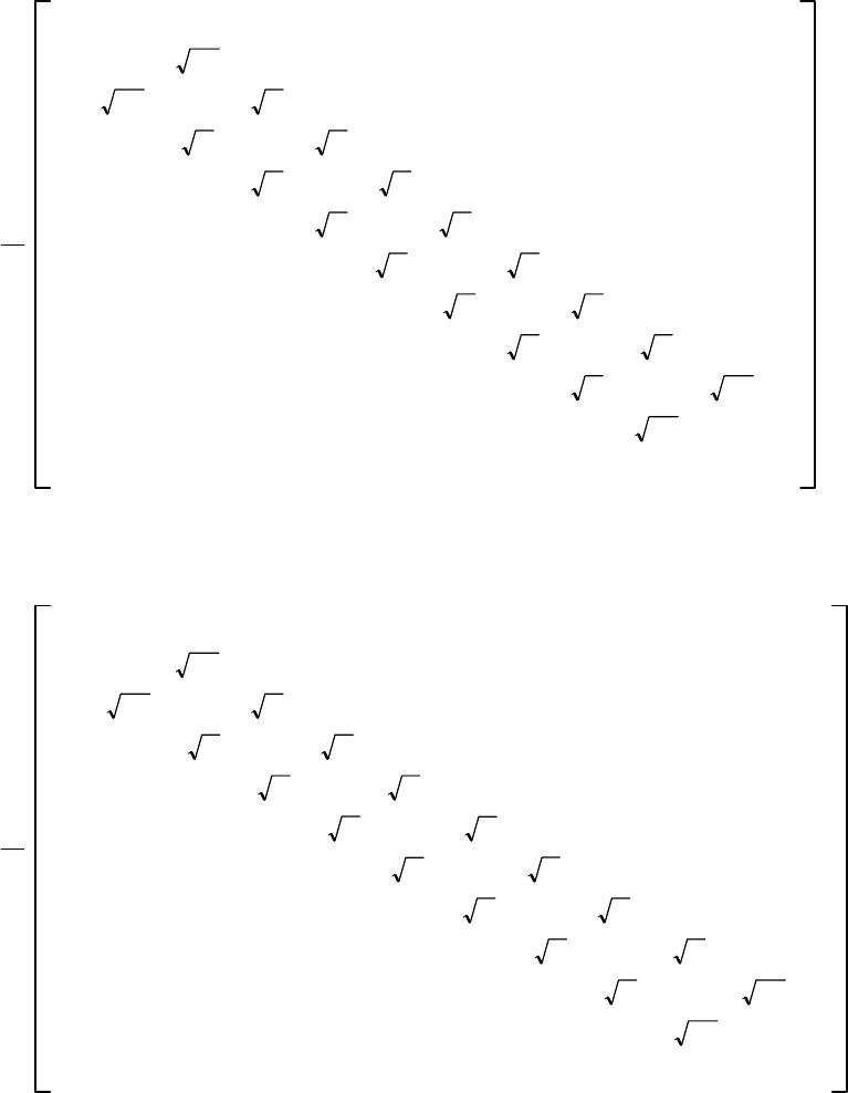 8Spin /2CSH {3/4,1/2,},j,1/2 Symbol{3/4, 1/2, }≡{23/4, n1/2, nn} Here j,1/2 ≡j,nn1/2 n≡j,1/2 (1) (2) The following are theconcrete expressions ofj,1/2 base on (6–1),(6–2),(6–3) Island operator 1,1/2 1 2 0i15 00 0 i150 i8 0 0i80 i3 00 i30 i0 i001 10i0 i00 i300 i30 i80 0i80 i15 000i150 (3) Island operator 2,1/2 1 2 015 00 0 –15 080 0–803 00 –300 –00-i1 i100 –003 –3080 0–8015 000–150 (4) 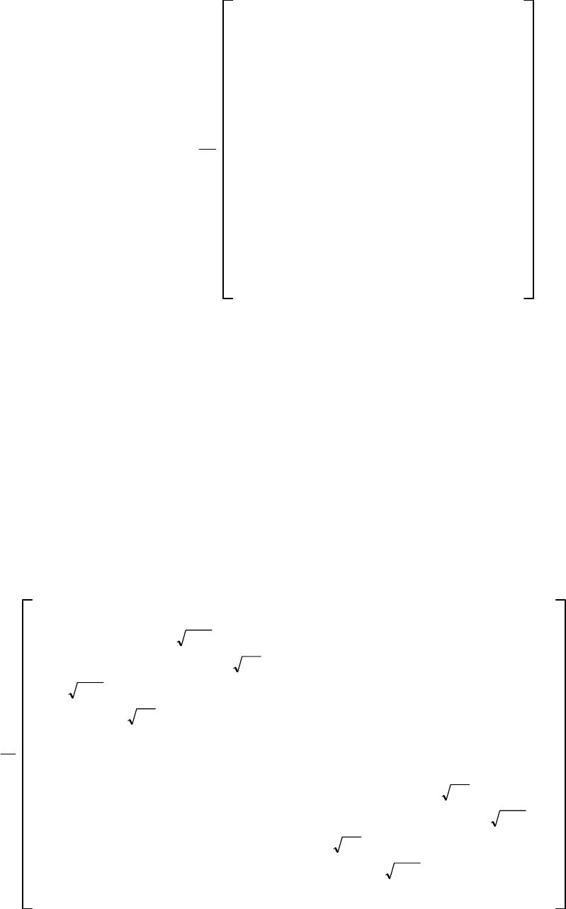 Island operator 3,1/2 1 2 9000 0 070 0 00 50 000 3 10 01 –3000 0–50 0 00 –70 0000–9 (5) The eigenvalues, from top left to down right, of Island operators 3,1/2 (5) are arranged from positiveinfinite to negative infinite. (3),(4),(5) obey angular momentum commutation relation j,1/2k,1/2 −k,1/2j,1/2 il,1/2,j,k.l1, 2, 3 (6) Evaluation of 1,1/2 2,2,1/2 2and 1,1/2 2 2,1/2 2 1,1/2 2 1 4 –390 -12000 0–230 -24 –120 0–11 0 0–24 0–3 10 01 −30-240 0−110 -120 –24 0−230 00–120 0−39 (7) 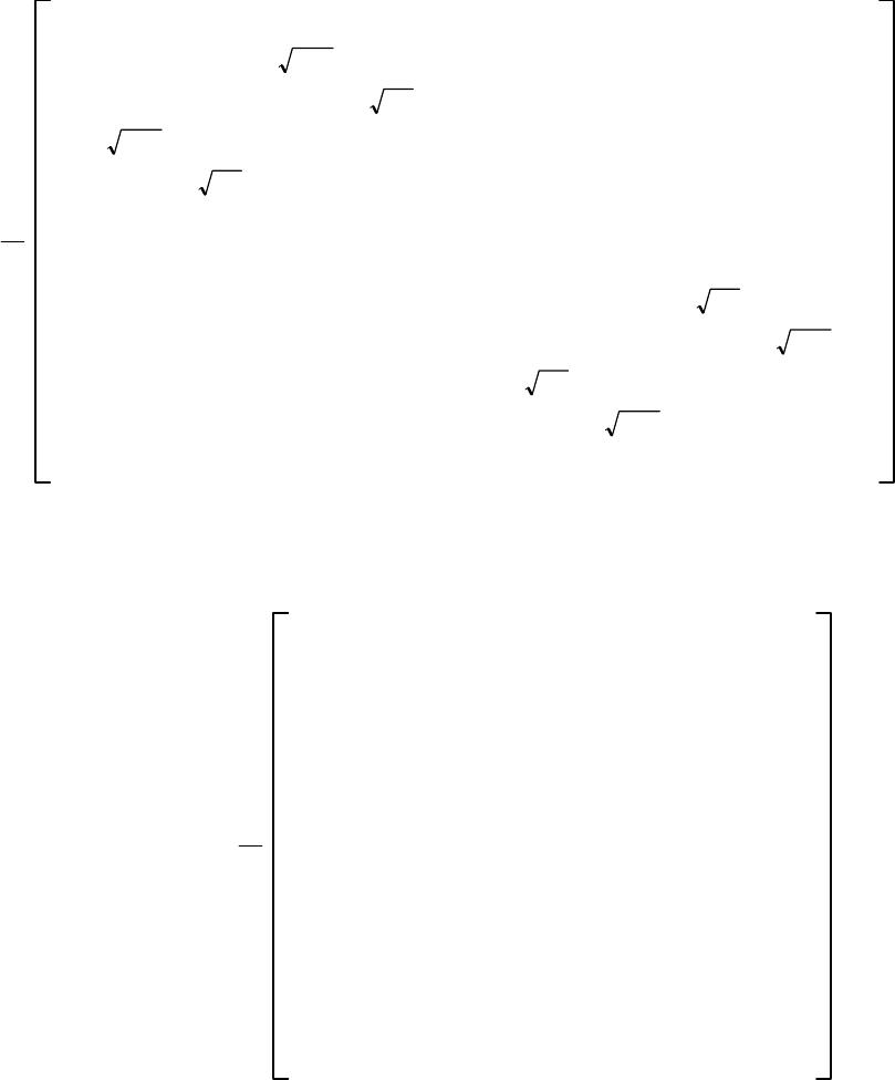 2,1/2 2 1 4 –390 12000 0–230 24 1200–11 0 024 0–3 10 01 −3024 0 0−110120 240−230 001200−39 (8) then obtain 1,1/2 2 2,1/2 21 4 −78 0000 0−46 00 00 −22 0 000 −6 20 02 −6000 0−22 00 00 −46 0 0000−78 (9)  3,1/2 21 4 81 0000 049 00 00 25 0 000 9 10 01 9000 025 00 00 49 0 000 081 (10) note Although the eigenvalues of 1,1/2 2 2,1/2 2(9) approach to negative infinite (from the matrix center where the eigenvalues are 1/2) in the direction of top left and down right, the eigenvalues of 3 2(10) are greater than1/4. Further the eigenvalues of total square operator 1/2 2(11) remains to be a finite number3 42. 1/2 2 1,1/2 2 2,1/2 2 3,1/2 23 421 21 212I0 (11) 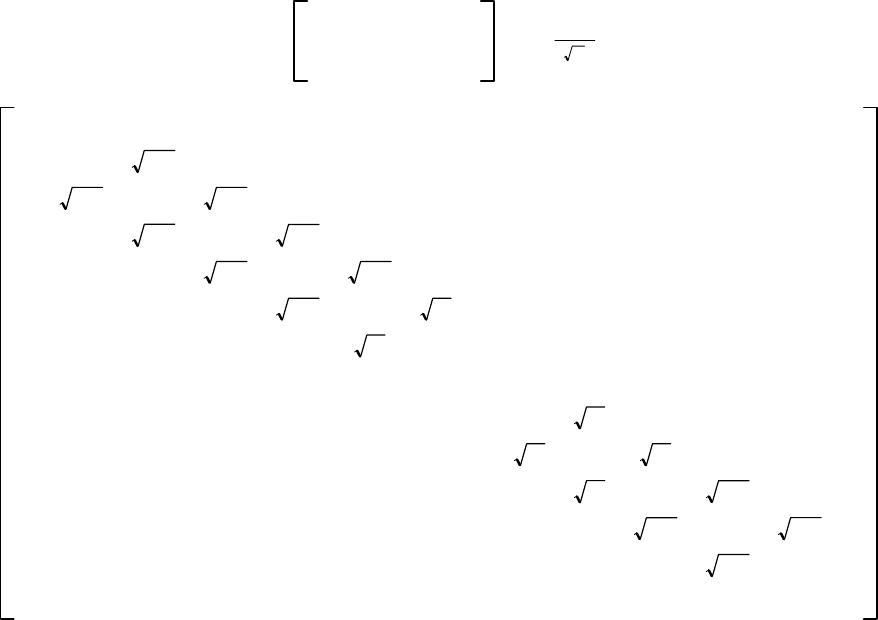 9Spin 1/3CSH {4/9,1/3,}, Δj,1/3 Symbol{4/9, 1/3, }≡{24/9, n1/3, nn} Here Δj,1/3 ≡Δj,nn1/3 n≡j,1/3 (1) (2) Ocean Operator: Δ1,1/3 1,4/3 U0 01,1/3 D1 6 0i500000 0 i500i34 000 0i340 i21 00 00i210 i11 0 000i110 i4 0000i400 0010000 10i1000 0i10 i600 00i60 i140 00 0i140 i25 000 00i250 (3)  Ocean Operator: Δ2,1/3 2,4/3 U0 02,1/3 D1 6 0500000 0 -50034000 0-3402100 00 -210110 000 -11 04 0000 -400 00−i00 00 i01 000 0-10600 00 -60140 00 0 -14025 000 00-250 (4) Ocean Operator: Δ3,1/3 3,4/3 U0 03,1/3 D 19/3000000 016/3 0000 00 13/3 000 000 10/3 00 0000 7/3 0 00000 4/3 0 01/3000 00 0 –2/3 0000 00 –5/3 000 000 –8/300 00 00–11/30 000 000–14/3 (5)  Obtain Δ3,1/3 2 256/9 00000 0169/9 000 00100/9 00 00049/9 0 000016/9 1/900 00 04/9 000 0025/9 00 00064/9 0 000 00121/9 (6) (3),(4),(5) obey angular momentum commutation relation Δj,1/3 2Δk,1/3 2−Δk,1/3 2Δj,1/3 2iΔl,1/3 2,j,k.l1, 2, 3 (7) We have Δ1,1/3 21 6 −840-714 00 0 0−550-231 0 -714 0−320-44 0-231 0−15 00 00-44 0−400 0010i100 0000-60 i10−70-84 0-60−200 000-840−39 (8)  Δ2,1/3 21 6 −840 714 00 0 0−550 231 0 714 0−320 44 0231 0−1500 0044 0−400 0010-i100 000060 -i10−7084 060−200 00084 0−39 (9) Obtain Δ1,1/3 2Δ 2,1/3 2 −252/900 0 00 0−165/90 0 0 00−96/9 00 000−45/9 0 0000−12/9 3/900 00 00 000 00−21/9 00 00 0−60/9 0 000 00−117/9 (10) Hence Δ1/3 2Δ 1,1/3 2Δ 2,1/3 2Δ 3,1/3 24 9I01 31 31I0 (11)  note Let us go backto Δ3,1/3(5). first note that Δ3,1/3 is an infinite dimensional diagonal matrix, from top left to down right,its eigenvalues are arranged from positive infinite to negative infinite. And its diagonal elements construct an arithmetic series, the difference between every two neighbour matrix elements of Δ3,1/3 are always integral number 1. Each matrix element on the principal diagonal of Δ3,1/3 2(6) is the positive real number. The least value is 1/9,that liesat the center of Δ3,1/3 2. Upwardtotop left side and downward to down right side of Δ3,1/3 2,the eigenvalues of Δ3,1/3 2 vary toward positive infinite. Δ1,1/3 2(8) and Δ2,1/3 2(9) are non-Hermitian matrices , but the sumΔ1,1/3 2Δ2,1/3 2 (10) of them is a Hermitian diagonal matrix,except 3/9 and 0,the rest of principal diagonal elements of (10) are all negative. Obviously, this result comes from the non-Hermiticityof matrices Δ1,1/3 and Δ2,1/3. Fortunately, the increasing speed of diagonal values of matrixelements of Δ3,1/3 2 (6), toward positive infinite, is slightly faster thanthat of Δ1,1/3 2Δ2,1/3 2(10) toward negative, that assures the total square spin angular momentum Δ1/3 2(11) to be a positive infinite dimensional diagonal matrix. There are only two diagonal matrix blocks for Ocean Operator. The difference between every twoadjacent elements of main diagonal of 3,1/3 (5) are always integral number 1,toa certainty, is same asthose of 3,0(7–8) and, 3,1/2(8–5) mentioned before. it is an essential regularity associated with CSH 3nn.  10Non-Hermitian MomentumP Phase Factor of Fractional Statistics 10.1 Non-Hermitian MomentumP Momentum andangular momentum are the most fundamental conceptsin quantum mechanics,which describe the linear motion and rotational motion of the particles in physics. After the disscussion of positive definite non-Hermitian self-adjoint angular momentum L,in this paragraph we turn to positive definite non-Hermitian self-adjoint momentum P. Hermitian MomentumPis defined as P1−isin cos∂r−i1 rcos cos ∂isin rsin ∂ P2−isin sin ∂r−i1 rcos sin ∂−icos rsin ∂ P3−icos ∂ri1 rsin ∂ (1.1) (1.2) (1.3) In spherical coordinates, we have the radial metric coefficient frr2, then the total metric coefficient of space is extended to three coordindate functions as follows (2) frgh;frr2,gsin14m0,h2T1 (2) Then take the Positive Definite Non-Hermitian Adjoint Operation of momentum (1.1),(1.2),(1.3) P1⊕isin cos ∂r ⊕i1 rcos ∂ ⊕cos −i1 rsin ∂ ⊕sin P2⊕isin sin ∂r ⊕i1 rsin ∂ ⊕cos 1 rsin ∂ ⊕cos P3⊕icos ∂r ⊕−i1 r∂ ⊕sin (3.1) (3.2) (3.3) Substitution of (2) into the adjoint representation of derivative operator (1–21) separately, yields the adjoint representins of derivative operator ∂r,∂,∂as follows ∂r ⊕−∂r−2 r ∂ ⊕−∂−14m0cot ∂ ⊕−∂−2T2 (4) (5) (6)  On using the (4),(5),(6), therefore P1⊕–isin cos∂r−i1 rcos cos ∂4m0cot −sin rsin l3–i2T2 P2⊕–isin sin ∂r−i1 rcos sin ∂4m0cot cos rsin l3–i2T2 P3⊕–icos ∂ri1 rsin ∂4m0cot (7.1) (7.2) (7.3) Because of P1⊕≠P1 P2⊕≠P2 P3⊕≠P3 (8.1) (8.2) (8.3) Consequently, the so-called well-definited momentumoperator in space (2), the positive definite non-Hermitian self-adjoint operator Pis introduced by following definition P1 2{P⊕P} (9) Then we have P1–isin cos∂r−i1 rcos cos ∂2m0cot −1 rsin sin L3 P2–isin sin ∂r−i1 rcos sin ∂2m0cot 1 rcos sin L3 P3–icos ∂ri1 rsin ∂2m0cot (10.1) (10.2) (10.3) After carefully evaluation, momentum square operator is writtenby P2P1 2P2 2P3 2Pr 21 r2L2 (11) Note where Pr−i∂r−i1 r L2−∂ 214m0cot ∂−sin −2L3 2−4m0 2−4m0 2−2m0 (12) (13) Here L2is what we have obtained in (2–19)namely, non-Heemitianorbital angular momentum square operator. 10.2By means of the orthonormal baseser,e,einspherical coordinates er sin cos sin sin cos ,e cos cos cos sin −sin ,e −sin cos 0 (14)  Using (14) to rewrite (10.1),(10.2),(10.3),we have (15) So P−ie r∂r−i1 re∂2m0cot 1 rsin eL3 (15) Position operatorr rre (16) On account of basis rules eree,eeer,eere er2e2er21 (17.1) (17.2) We concludecross productrPof position operatorr(16) with momentum operator P(15), obtain rP rer−ie r∂r−i1 re∂2m0cot 1 rsin eL3 0−i1 re∂2m0cot −1 sin eL3 (18) (19) and three components of (18) are rP1isin ∂2m0cot −cot cos L3 rP2−icos ∂2m0cot −cot sin L3 rP3−i∂−iT2 (20.1) (20.2) (20.3) Comparing (20.1), (20.2),(20.3) with (2–13), (2–14), (2–15),we see that the definition rP(18) is namelypositive definite non-Hermitian self-adjoint orbital angular momentum previously obtained. rP≡L L−i −sin cos 0 ∂2m0cot −1 sin cos cos cos sin −sin L3 (21) (22) Next we will use non-Hermitian momentumoperatorPto give some interesting and heuristic ideas whichrelated to gauge invariance in space (2) and the phase factor of fractional statisticsof particle wavefunctions.  10.3 The Gauge Invariance in Spacefrgh a) Non-Hermitian momentum P(15) can be expressed by derivative f. P−if (23) Where fer∂r1 re∂2m0cot i1 rsin eL3 ∂1 re2m0cot 1 rsin eT2 f∂ (24) (25) Where ∂−ie r∂r−i1 re∂1 rsin el3 1 re2m0cot 1 rsin eT2 (26) (27) If no confusion, we use symbol∇∂.The components of as follows r0, 2m01 rcot ,1 rsin T2 sin 1 rT2 r1 sin T2 r2m0cot (28) (28.1) (28.2) (28.3) Using the above results to evaluate∇, obtaim ∇1 rsin ∂sin −∂ er 1 r1 sin ∂r−∂ rr e 1 r∂rr−∂ r e 1 rsin ∂1 rT2−∂ 2m01 rcot er 1 r1 sin ∂0−∂ r1 sin T2 e 1 r∂r2m0cot −∂ 0 e 0 (29) (30) further ∇0 f∇ 0 (31) (32) (31) and (32) show that isirrotational field respect to ∇and derivative f.  b) In space (2), Schro ̈dinger equation and minimal coupling theorem are defined as P−e cA2ei∂t (33) Using(25),have −2 2m f−ie cA2ei∂t −2 2m D2ei∂t (34) (35) where D≡f−ie cA (36) Dis called the covariantderivative of wave function respect tothe gauge vector potential Ain space (2). By means of gauge transformation (37),(38) x′xexp [ie cx]x AjxAj ′xAjx∂jx (37) (38) here ie cxis phase factorof wave function xas follow x x0C x ADl (39) where Dl is differential length [cf.(60)] Wemakefollowinggauge transformations ofcovariant derivative Djand wavefunction . Djx{fj−ie cAj}x{∂jj−ie cAj}x Dj ′′x{fj−ie cAjx∂jx }expie cx x {∂jj−ie cAjx∂jx }expie cx x exp ie cx {∂jie c∂jx j−ie cAjx∂jx }x exp ie cx{∂−ie cAjx}x exp ie cx{fj−ie cAjx}x Dj ′′xexp ie cx{fj−ie cAj}x Dj ′′xexp ie cx Djx (40) (40.1) (40.2) (41) (42)  Using (41),(42), Further Dj 2x{fj−ie cAj}2x{∂jj−ie cAj}2x Dj ′2′x{fj−ie cAjx∂jx }2exp ie cx x {∂jj−ie cAjx∂jx }2exp ie cx x {∂jj−ie cAjx∂jx } {∂jj−ie cAjx∂jx }exp ie cx x {∂jj−ie cAjx∂jx } expie cx{fj−ie cAj}x[using (40.1), (40.2)] expie cx {fj−ie cAj}{fj−ie cAj}x Dj ′′xexp ie cx Dj 2x (43) (44) Then using (44) and (35), we have {−2 2m D′2e}′exp ie cx {−2 2m D2e}(44) exp ie cx i∂t(35) i∂t′i∂t{expie cx }i∂t′ (45) (46) (47) So the gaugeinvariance of Schro ̈dinger equation in space (2) is demonstrated by the above expatiation. 10.4 Phase Factor of Fractional Statistics Then focus our attentation on the phase factor of fractional statistics by using line integral on (42) for any closed counterclockwise loop C, encircling the origin, which is the most fascinating phenomenon of line path integral (67). c) As a matterof convenience, in the next paragraph use ec1.Now we will consider with a special gauge vector potential Aofwave function xin space (2) as A1 2rsin e (48) we see Ais an irrotationalfield ∇A1 rsin ∂sin 1 2rsin −∂ 0 er 1 r1 sin ∂0−∂ rr1 2rsin e 1 r∂rr0−∂ 0 e46 ∇A0 (49) (50) 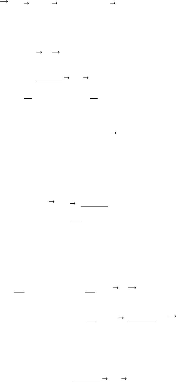 In space (2), differential length is defined as Dl erdr ersin4m0dersin hd (51) Using (39), evaluating factor xintegral x x0C x ADl (39) C 1 2rsin eersin hd 1 2Chd1 2Cd2T1 xI014m0I012nI0 (52) (53) (52) shows the contour integral of gauge vector Ais directly connected with the spin quantum numbers nof particles of CSH!without any phenomenological postulation. d) For clearer,resume physical units, gauge potential (48) turns to(54) Ae1 2rsin c e0/2 (54) (55) where 0isfundamental magnetic flux. According to (37), the period of phase factor of wavefunction are written as exp ie cx exp ie c C x ADl exp ie c C x e1 2rsin Dl (56) (57) take to be fundamental magnetic flux 0,and use (37),(39),(53),(57), we have xxexp [iC 1 2rsin eersin hd] xexp [ i12nI0] (58) (59)  e) Using (59), make classfication of spinparticles by quantun number n. 1) For Bosons: nn,are integers, such 0,1, 2, 3,..., then phase are ,3,5,7....; nn−,are integers, such 0,−1, −2, −3,..., then phase are ,−,−3,−5.... 2) For Fermions: nn,are half-integers, such 1/2, 3/2, 5/2, 7/2..., then phase are 2,4,6,8....; nn−,are half-integers, such −1/2, −3/2, −5/2, −7/2,..., then phase are 0,−2,−4,−6.... We see all Bosons lie at the negative real coordinate axis andall Fermions lie at the positive real coordinate axis 3) For TKP:nand n−are neither integers nor half-integers. nn,are1/3, 2/3,...,then phase are 5/3, 7/3/3,....; nn−,are−1/3, −2/3,...,then phase are /3, −/3,.... nn1/4,then phase is 3/2; nn−−1/4,then phase is /2. We can choose different vector potential A,for different physical pictures in space (2), thenwe will have different represents of (59) or(37). 10.5 The Third Kind of Particles, TKP are not Anyons cite: [5] 1) The generators of Anyons do not satisfy the commutation rules of angular momentum, so Anyons are not real spin particles; The generatorsof TKP obey angular momentum commutation relations, they are true spin particles. 2) Anyons are classified according to braind group BN;TKP are the extension of groups SO3and SU2. 3) Anyons exist only in two dimensional system; TKPare exist in three dimensional system. 4) Anyons do not depend on space metric, that be formulated from topological quantum field theory; The physical concepts of TKP arise fromangular momentum, which are tightly connected with the three-dimensional space construction.  11 Conclusion Now back to chapter0,in conventional quantum mechanics, the eigenvalues of total square operator J2of spin angular momentum are expressed by (0-23) and the representations of matrix dimensionality Dof spin angular momentumare related to the values of the spin particles as shownwith formula (0-24). Note It is seen, that due to the eigenvalues of the third component matrix J3 could extend to , formulae (0-23) and (0-24) are untenable ! as follow 1) For an example, in conventional quantummechanics,max is integer and half-integer in the dimensionality formulaD(0-24). We see,the less the value of max,thesmall the matrix dimensionality of spin angular momentum.From spin 1, tospin/2,tospin0,the dimensionality is 3, to, 2, to 1. What will happen? if max continues to decrease in interval (/2, 0). If max spin /3,spin /4,spin /5,spin /6,... Then D2max 12/3 1, 2/4 1, 2/5 1, 2/61,... 5/3,6/4,7/5,8/6,... dimensionality Dis fractional ! This means that if formula (0-24) were still valid, you should construct so-called fractional-matrix !which is imcompatible with the skeleton frame of the present math, at least.So there are only two kinds of spin particles in conventional quantum mechanics. Whereas, afterthe exposition of chapter5andchapter 6, and later three examples of typicalspin particles of CSP (chapters 7,8,9),it is shown that in the system of Chaos Spin Hierarchy, the dimensionalities Dof spin 0/2, /3 extend to infinite! Actually, in Chaos Spin Hierarchy (in chapter 6),all the membersof spin angular momentum, 1,n (6-1),(6-5), 2,n (6-2),(6-6), 3,n (6-3),(6-7) and (n 2 (6-4),(6-8) are expressed by infinite matrices, which are indenpendent of the spin values of the particles. Further the axiom (0-24)should be abandoned. If we want to still hold down the (0-24), after all,D2max 1,in this sense, that seems to somewhat "reasonable". 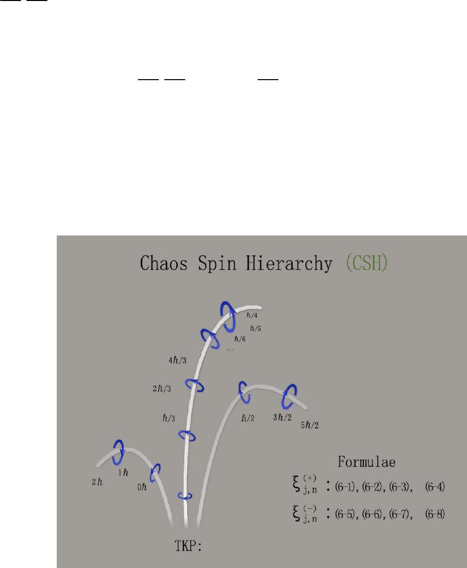 2) When extends to max ,further formula (0-23) that concerns about the eigenvalue of total square operator J2of spin angular momentum,is invalid too. Actually, in Chaos Spin Hierarchy, ther are two dimensionality formula (6-4) and (6-8) which highly resemble (0-23) maxmax 1k/2 k/2 1nn1nn1n 2 (0-23) (6-4), (6-8) But their derivations are quite different: a) In (0-23), the eigenvalue of total square operator J2is symboled by k/2 k/2 1that be derived from maxmax 1.Heremax is the maximum of J3in conventional mechanics,corresponds to quantumnumber m. b) (6-4), (6-8) represented by quantumnumber n2m0(4-7), n−−2m0(4-8). Here 2m0is a parameter that depicts the curvature of spacehg(2-5), which initially appears in the eigenvalue expressions m2m0of non-Hermitian angular momentum L3. This paper shows how Non-Hermitian angular momentum. comes towhat TKP is today Author places some hope on the adoptionabove, to give a good deal of enlightenment for both students and researchers, and wish the formulations of TKP is compatible with the axiomatic of quantum mechanics knownas yet,further an idea in theuses of future physics. In this paper, some fundamental research, which results in non-Hermitian angular momentum (both orbit and spin) of author’s work for past years, are givencite: [3],[4]. TKP methodology is applied to Energy Harmonic Oscillator Hierarchy (EHOH) and infinite dimensional matrices of Lorentz Group,much of which have never beenpublishedinpublicjournalsbeforecite: [3]. This article mainly comes from author’s English-Lectures that designed to serve the needs of workshop and seminar in China. ACKNOWLEDGEMENT Author thanks Yong-Shi Wu, Professor of University of Utah USA, for his helps and encouragements REFERENCES [1] Bender C M, Boettcher S, F.G Scholtz, H.B Geyer, F. Hahne, A.Mostafazadeh, C. Figueira de Morisson Faria, Wu Jund and A.Fring, H.F.Jones, M.Znojil. [2] A.Mostafazadeh 2002 J.Math.Phys. 43 205 2814, 3944 [3] ShaoXu Ren,Advanced Non-Euclidean Quantum Mechanics ISBN 978-7-80703-585-4(2006) ; Frontier Science ISSN 1673-8128.vol 2, (2008); vol 5,(2011) ; The Third Kind of Particles ISBN978-7-900500-91-5(2011) ; The Third Kind of Particles ISBN978-988-15598-9-0(2012) ; The Third Kind of Particles ISBN978-3-659-17892-4(2012) ; Faster Than Velocity Of Light ISBN978-988-12266-2-4(2013) . [4] ShaoXu Ren,Scientific Programm of the ICAP 2006-20th International Conference on Atom Physics, Innsbruck, Austria. [5] Leinaas, J.M.; J. Myrheim(11 January 1977). Onthe theory of identical particles. Il Nuovo Cimento B37(1): 1–23. Wilczek, Frank (4 October 1982). Quantum Mechanics of Fractional-Spin Particles. Physical ReviewLetters 49 (14): 957–959. 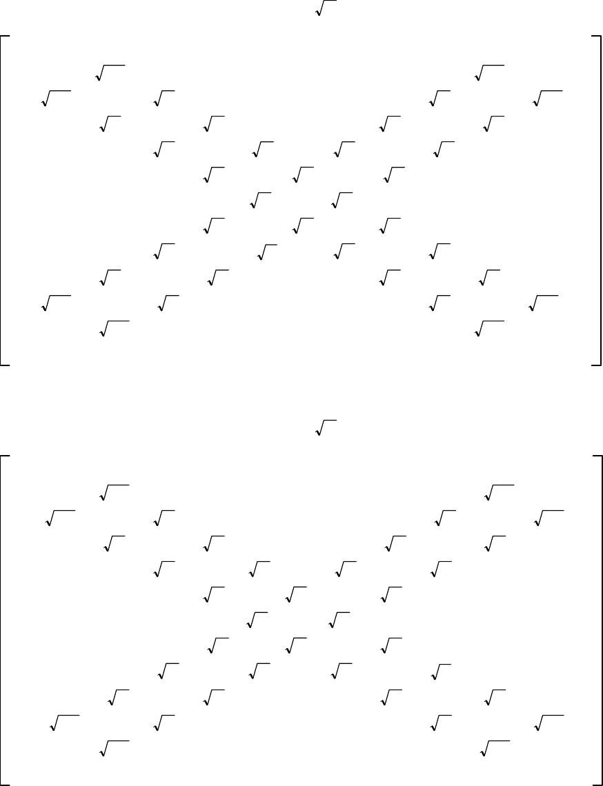 Appendix: Infinitesimal Rotation of TKP A1) Infinitesimal Rotationof Particle of Spin 0CSH Infinitesimal rotation operatorW1,01/2 0i10000 i100 i100 i600 i60–i10 i60 i3 0i30–i6 i30 i1i10–i3 i1000–i1 000 i1000i1 i30–i1i10 i3 i60–i3i30i6 i10 0–i6i60 i10 0–i10 i100 (1) Infinitesimal rotation operatorW2,01/2 0i10 –i100 i100 i6 –i60 i10 i60 i3 –i30i6 i30 i1 –i10 i3 i1000i1 000 –i1000i1 –i30i1i10 i3 –i60i3i30 i6 –i100i6i60 i10 0i10 i100 (2) 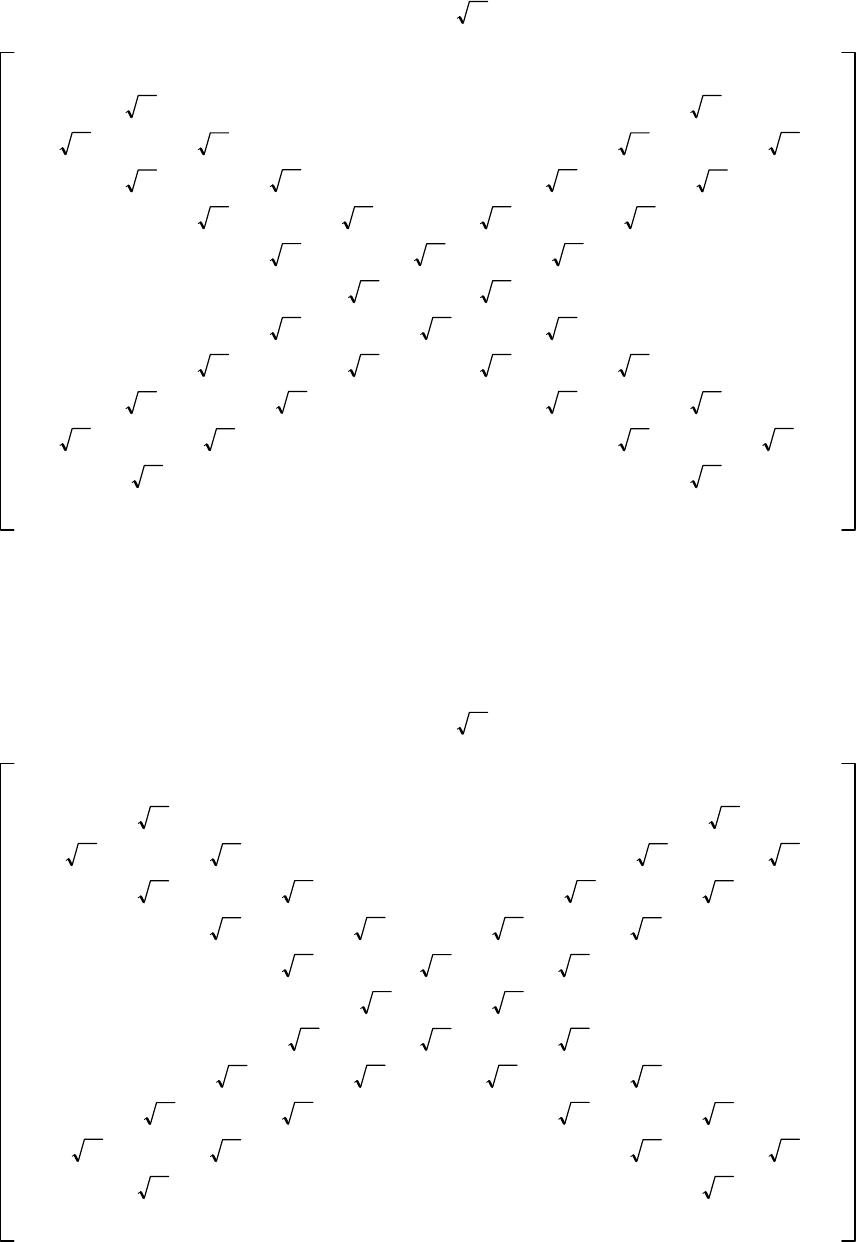 A2) Infinitesimal Rotationof Particle of Spin 1CSH cite: [3] Infinitesimal rotation operatorW1,11/2 0i9i90 i90i5i50–i9 i50 i2i20–i5 i20 i0i00–i2 i00 i10–i0 –i10 i1 i00–i10 i0 i20–i0i00 i2 i50–i2i20 i5 i90–i5i50i9 0–i9i90 (3) Infinitesimal rotation operatorW2,11/2 0i9 –i90 i90 i5 –i50 i9 i50 i2 –i20 i5 i20 i0 –i00 i2 i00 i10 i0 –i10–i1 –i00i10 i0 –i20 i0i00i2 –i50 i2i20 i5 –i90i5i50 i9 0i9i90 (4) 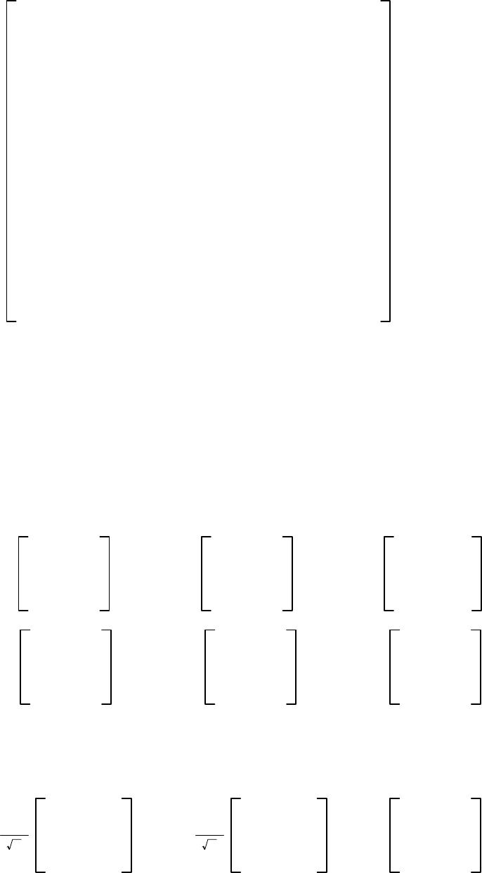 A3)ParticleofSpin0CSH and Particle of Spin 1CSH have the same math figure in their third Infinitesimal Rotation operators, that is W3,0 0−5i 0−4i 0−3i 0−2i 0−i 0 i0 2i0 3i0 4i0 5i0 W3,1 (5) Operators Wj,nobey angular momentum commutation rules Wj,nWk,n−Wk,nWj,niWl,n (6) Here space indexes j,k,l1, 2, 3arecirculative; particle spin quantum numbers n0, 1 A4) Operators Sj,Fj,Wjare 33matrices. S1 00 0 00–i 0i0 ,S2 00i 000 –i00 ,S3 0−i0 i00 000 F1 0i0 –i00 000 ,F2 00 0 00–i 0i0 ,F3 00–i 00 0 i00 (7) (8) SjSk−SkSjiSl FjFk−FkFjiFl (9) (10) W11 2 0i0 –i0i 0–i0 ,W21 2 0i0 –i0–i 0i0 ,W3 00–i 00 0 i00 (11) WjWk−WkWjiWl (12) In case of Spin 1CSH, we select Wjas the matrixcenter parts of Wj,1, due to the most symmetrical design of the math harmony of Infinitesimal rotation of TKP.Operators Fj,Wjwill be chosen as the center of Wj,nin other physical pictures.  Scientific Research Publishing (SCIRP) is one of the largest Open Access journal publishers. It is currently publishing more than 200 open access, online, peer-reviewed journals covering a wide range of academic disciplines. SCIRP serves the worldwide academic communities and contributes to the progress and application of science with its publication. Other selected journals from SCIRP are listed as below. Submit your manuscript to us via either |