Study on Psychological Crisis Evaluation CombiningFactor Analysis and Neural Networks

doi:10.4236/psych.2011.22022

Paper Menu >>

Journal Menu >>

Psychology

2011. Vol.2, No.2, 138-142

Study on Psychological Crisis Evaluation Combining

Factor Analysis and Neural Networks*

Hui Lin1, Yingbi Zhang1, Hengqing Tong1, Qiaoling Tong2, Dongsheng Liu2

1Department of Mathematics, Wuhan University of Technology, Wuhan, China;

2Department of Electronic Science & Technology, Huazhong University of Science & Technology,

Wuhan, China

Email: [email protected], [email protected]

Received August 17th, 2010; revised December 16th, 2010; accepted January 15th, 2011.

Effective and rapid psychological crisis evaluation under emergency is the basis to carry out psychological crisis

intervention (PCI). In this paper, based on existing research, an index system to evaluate the state of psycho-

logical crisis is established and the index system is simplified by the model combining factor analysis and neural

networks. Experiments illustrate that the training times, training time and maximum error of the combination

model are 1445, 20.476 (s), 0.0011 respectively while the general neural networks are 5581, 115.610 (s), 0.0090

with 92 samples and the final diagnosis by the combination model are also exact.

Keywords: Psychological Crisis, Evaluation, Inde x S ystem, Factor Analysis, Neural Networks

Introduction

In 1964, American psychologist G. Gaplan originally brought

up psychological crisis (PC). He defined psychological crisis as

the status of psychological unbalance in which individuals

could neither avoid nor cope with sudden or serious life events

(Gaplan, 1964). Once the psychological crisis occurs, the psy-

chological crisis intervention (PCI) is needed immediately to

recalibrate the mental situation to normal level, in case the in-

dividuals fall into a status of suffering, anxiety, coupled with

desperation, autonomic symptoms and behavior disorder.

However, the effective crisis intervention is dependent on ac-

curate evaluation. Through evaluation, the psychologist can

understand the individuals’ crisis situation and their reactions

thus effective crisis intervention can be carried out as soon as

possible.

Myer and Williams (1992) proposed a three-dimensional tri-

age evaluation model which provides a framework for under-

standing individuals’ reactions during a crisis. The model pre-

sumes that reactions to crisis events are seen in three domains:

cognitive, affective and behavioral (Myer, William, Ottens &

Schmidt, 1992). Brende (1998) presented an evaluation model

of phases based on his research on unprecedented and destruc-

tive floods from 1987 to 1998 in USA. In this article he says

that survivors’ predictable emotional and physiological re-

sponses usually process through five phrases over a period of

time toward either resolution or symptom development. To

preclude more severe and chronic symptoms, survivors should

be debriefed by trained professionals within 48 hours (Brende,

1998). Wilson (1999) brought up a person-envi- ronment inter-

actional model to explain the typologies of traumatic events and

stressor dimensions. This model pays attention to comprehen-

sion of stress and its factors as well as the diversity of traumatic

events (Wilson, 1999).

In this article, we propose a novel and effective method to

evaluate PC. Firstly integrating the core idea of Myer and Wil-

liams, we establish an evaluation index system for psychologi-

cal crisis. Further, considering the evaluation should be effec-

tive and valid, we put forward an evaluation model combining

factor analysis and back-propagation neural networks. Through

factor analysis, the intrinsic relationships among indices are

eliminated, and the dimension of these indices is compressed

while enough information is maintained. Moreover, the struc-

ture of the neural networks is simplified. Overall, the accuracy

of networks’ output is improved and the evaluation time is re-

duced.

Establishing Evaluation Index System

Evaluation index system has monitoring function which

adopts one or more rigorous theories to analyze the causal rela-

tionship between individuals and development of crisis accord-

ing to the status of the individuals.

The three-dimensional triage evaluation model proposed by

Myer and Williams is considered to be a simple and rapid

evaluation system. While in a state of emergency, it also re-

quires that the evaluation and the diagnosis should be accurate;

therefore the article starts to establish an evaluation index sys-

tem to evaluate the state of psychological crisis.

When individuals face a crisis, they will conduct a series of

physical and psychological reactions, and the reactions to the

crisis are mainly in physical, emotional, cognitive and behav-

ioral domains. Accordingly, the psychological crisis evaluation

index system can be established from these four domains. The

index system is shown in Table 1.

Using a 90-item self-report symptom inventory (SCL-90) for

reference, we divide each specific index of the evaluation index

system into five levels: not at all, a little bit, moderately, quite a

bit, extremely (Holi, 2003). Each level is assigned a score from

*The project was supported by the National Natural Science Foundation o

China (305 70611, 60773210).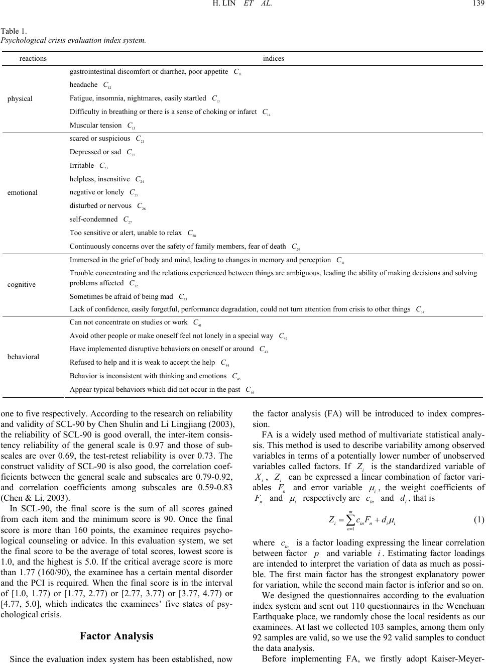

H. LIN ET AL. 139

Table 1.

Psychological crisis evalu a tion index system.

reactions indices

gastrointestinal discomfort or diarrhe a, poor appetite

headache

Fatigue, insomnia, nightmares, easily s t ar t l ed

Difficulty in breathi ng or there is a sense of choking or in f arct

physical

Muscular tension

scared or suspicious

Depressed o r sad

Irritable

helpless, insensitive

negative or lonely

disturbed or nervous

self-condemned

Too sensitive or alert , unable to r elax

emotional

Continuously concerns over the safety of family members, fear of death

Immersed in the grief of body and mind, leading to changes in memory an d p erception

Trouble co n centrating and the rel ations expe r ienced between things are ambiguous, leading the ability of making decisions a nd solving

problems affected

Sometimes be afraid of being mad

cognitive

Lack of co n fi d ence, easily forgetful, performance degradation, could not turn atten t ion from crisis to other things

Can not conc entrate on studies or work

Avoid other people or make oneself feel not lonely in a special way

Have implemented disruptive behaviors on o n eself or around

Refused to he l p and it is weak to accept the help

Behavior is inconsistent with think ing and emotions

behavioral

Appear typ i cal behaviors which did not occur i n th e past

one to five respectively. According to the research on reliability

and validity of SCL-90 by Chen Shulin and Li Lingjiang (2003),

the reliability of SCL-90 is good overall, the inter-item consis-

tency reliability of the general scale is 0.97 and those of sub-

scales are over 0.69, the test-retest reliability is over 0.73. The

construct validity of SCL-90 is also good, the correlation coef-

ficients between the general scale and subscales are 0.79-0.92,

and correlation coefficients among subscales are 0.59-0.83

(Chen & Li, 2003).

In SCL-90, the final score is the sum of all scores gained

from each item and the minimum score is 90. Once the final

score is more than 160 points, the examinee requires psycho-

logical counseling or advice. In this evaluation system, we set

the final score to be the average of total scores, lowest score is

1.0, and the highest is 5.0. If the critical average score is more

than 1.77 (160/90), the examinee has a certain mental disorder

and the PCI is required. When the final score is in the interval

of [1.0, 1.77) or [1.77, 2.77) or [2.77, 3.77) or [3.77, 4.77) or

[4.77, 5.0], which indicates the examinees’ five states of psy-

chological crisis.

Factor Analysis

Since the evaluation index system has been established, now

the factor analysis (FA) will be introduced to index compres-

sion.

FA is a widely used method of multivariate statistical analy-

sis. This method is used to describe variability among observed

variables in terms of a potentially lower number of unobserved

variables called factors. If i

is the standardized variable of

can be expressed a linear combination of factor vari-

ables n

and error variable i



, the weight coefficients of

and i



respectively are and , that is

iinni

cF d







 (1)

where in is a factor loading expressing the linear correlation

between factor and variable . Estimating factor loadings

are intended to interpret the variation of data as much as possi-

ble. The first main factor has the strongest explanatory power

for variation, while the second main factor is inferior and so on.

cpi

We designed the questionnaires according to the evaluation

index system and sent out 110 questionnaires in the Wenchuan

Earthquake place, we randomly chose the local residents as our

examinees. At last we collected 103 samples, among them only

92 samples are valid, so we use the 92 valid samples to conduct

the data analysis.

Before implementing FA, we firstly adopt Kaiser-Meyer-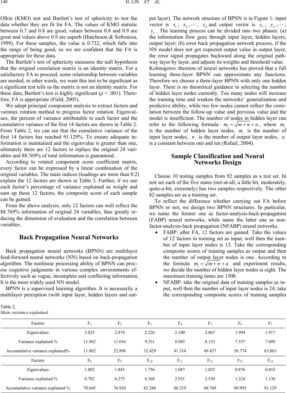

H. LIN ET AL.

140

Olkin (KMO) test and Bartlett’s test of sphericity to test the

data whether they are fit for FA. The values of KMO statistic

between 0.7 and 0.8 are good, values between 0.8 and 0.9 are

great and values above 0.9 are superb (Hutcheson & Sofroniou,

1999). For these samples, the value is 0.732, which falls into

the range of being good, so we are confident that the FA is

appropriate for these data.

The Bartlett’s test of sphericity measures the null hypothesis

that the original correlation matrix is an identity matrix. For a

satisfactory FA to proceed, some relationship between variables

are needed, in other words, we want this test to be significant as

a significa nt test tell s us the matrix is not an identity matrix. For

these data, Bartlett’s test is highly significant (p < .001). There-

fore, FA is appropriate (Field, 2005).

We adopt principal component analysis to extract factors and

varimax rotation method to progress factor rotation. Eigenval-

ues, the percent of variance attributable to each factor and the

cumulative variance of the first 14 factors are shown in Table 2.

From Table 2, we can see that the cumulative variance of the

first 14 factors has reached 91.129%. To ensure adequate in-

formation is maintained and the eigenvalue is greater than one,

ultimately there are 12 factors to replace the original 24 vari-

ables and 88.769% of total information is guaranteed.

According to rotated component score coefficient matrix,

every factor can be expressed by a linear combination of the

original variables. The main indices (loadings are more than 0.2)

explain the 12 factors are shown in Table 3. Further, if we use

each factor’s percentage of variance explained as weight and

sum up these 12 factors, the composite score of each sample

can be gained.

From the above analysis, only 12 factors can well reflect the

88.769% information of original 24 variables, thus greatly re-

ducing the dimension of evaluation and the correlation between

variables.

Back Propagation Neural Networks

Back propagation neural networks (BPNN) are multilayer

feed-forward neural networks (NN) based on back-propagation

algorithm. The nonlinear processing ability of BPNN can proc-

ess cognitive judgments in various complex environments ef-

fectively such as vague, incomplete and conflicting information.

It is the most widely used NN model.

BPNN is a supervised learning algorithm. It is necessarily a

multilayer perception (with input layer, hidden layers and out-

put layer). The network structure of BPNN is in Figure 1: input

vector is 1

, 2

,, m

and output vector is 1, 2,,

n. The learning process can be divided into two phases: (a)

the information flow goes through input layer, hidden layers,

output layer; (b) error back propagation network process, if the

NN model does not get expected output value in output layer,

the error signal propagates backward along the original path-

way layer by layer, and adjusts its weights and threshold value.

y y

Kolmogorov theorem of neural networks has proved that a full

learning three-layer BPNN can approximate any functions.

Therefore we choose a three-layer BPNN with only one hidden

layer. There is no theoretical guidance in selecting the number

of hidden layer nodes currently. Too many nodes will increase

the training time and weaken the networks’ generalization and

predictive ability, while too few nodes cannot reflect the corre-

lation between the follow-up value and previous value and the

model is insufficient. The number of nodes in hidden layer can

refer to the following formula: 1

mmna, whe1

is the number of hidden layer nodes, 1

m is the number of

input layer nodes, n is the number of output layer nodes, a

is a constant between one and ten (Rafael, 200

 re

4).

Sample Classification and Neural

Networks Design

Choose 10 testing samples from 92 samples as a test set. In

test set each of the five states (not-at-all, a little bit, moderately,

quite-a-bit, extremely) has two samples respectively. The other

82 samples are as a training set.

To reflect the difference whether carrying out FA before

BPNN or not, we design two BPNN structures. In particular,

we name the former one as factor-analysis-back-propagation

(FABP) neural networks, while name the latter one as non-

factor-analysis-back propagation (NFABP) neural networks.

 FABP: after FA, 12 factors are gained. Take the values

of 12 factors in training set as input, well then the num-

ber of input layer nodes is 12. Take the corresponding

composite scores of training samples as output and then

the number of output layer nodes is one. According to

the formula 1

mmna



 and experiment results,

we decide the number of hidden layer nodes is eight. The

maximum training times are 1500.

 NFABP: take the original data of training samples as in-

put, well then the number of input layer nodes is 24; take

the corresponding composite scores of training samples

Table 2.

Main variance explained.

Factors F1 F

2 F

3 F

4 F

5 F

6 F

Eigenvalues 3.025 2.874 2.226 2.100 2.067 1.994 1.917

Variance explained % 11.882 11.016 9.531 8.885 8.123 7.337 7.089

Accumulative variance explained% 11.882 22.898 32.429 41.314 49.437 56.774 63.863

Factors F8 F

9 F

10 F

11 F

12 F

13 F

Eigenvalues 1.882 1.843 1.756 1.087 1.052 0.876 0.853

Variance explained % 6.782 6.275 6.368 2.931 2.550 1.224 1.136

Accumulative variance explained % 70.645 76.920 83.288 86.219 88.769 89.993 91.129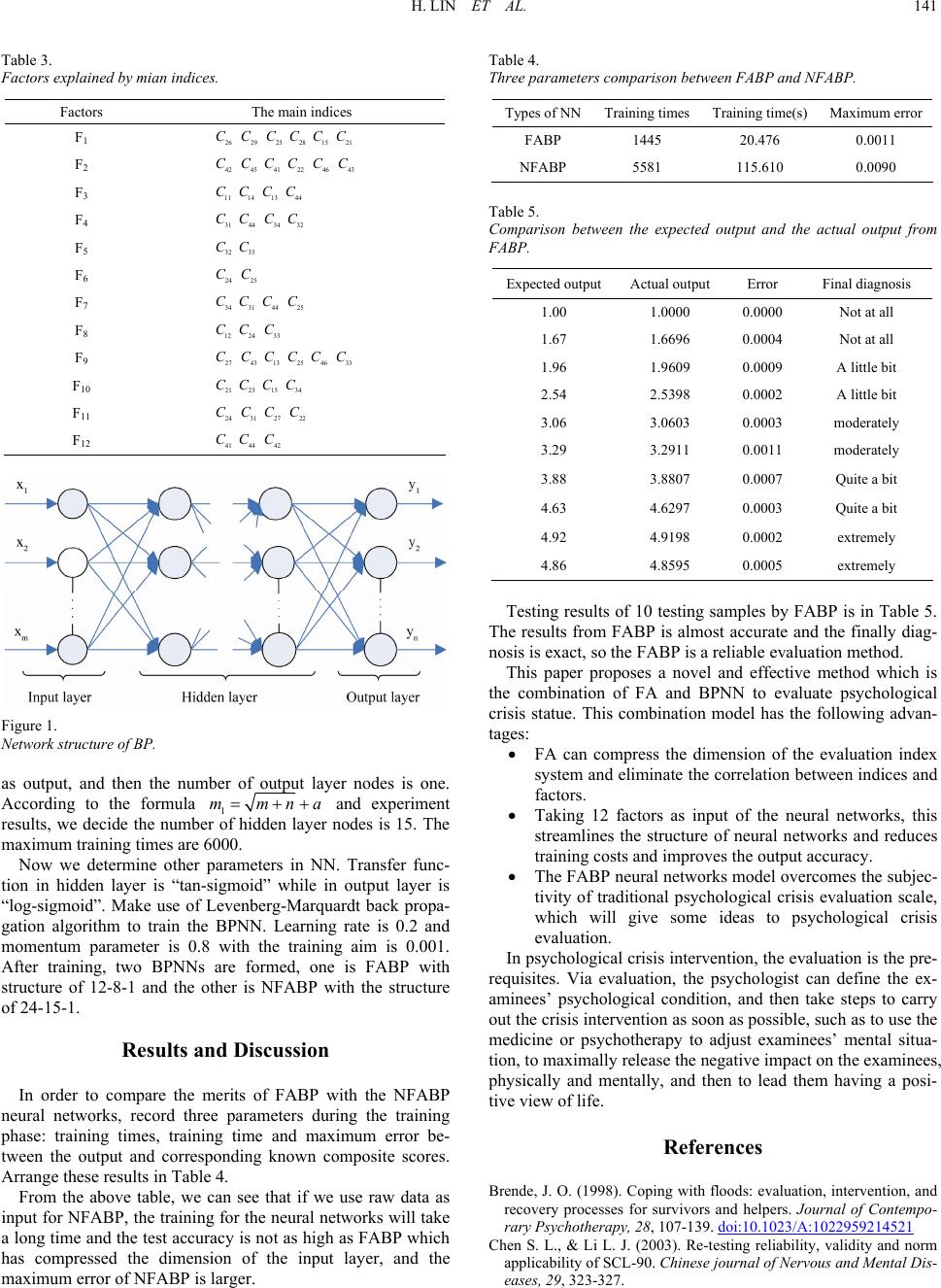

H. LIN ET AL. 141

Table 3.

Factors explained by mian indices.

Factors The main indices

F1 26

C29

C23

C28

C15

C21

F2 42

C45

C41

C22

C46

C43

F3 11

C14

C13

C44

F4 31

C44

C34

C32

F5 32

C33

F6 24

C25

F7 34

C31

C44

C25

F8 12

C24

C33

F9 27

C43

C13

C25

C46

C33

F10 21

C23

C15

C34

F11 24

C31

C27

C22

F12 41

C44

C42

Figure 1.

Network structure of BP.

as output, and then the number of output layer nodes is one.

According to the formula 1

mmna



 and experiment

results, we decide the number of hidden layer nodes is 15. The

maximum training times are 6000.

Now we determine other parameters in NN. Transfer func-

tion in hidden layer is “tan-sigmoid” while in output layer is

“log-sigmoid”. Make use of Levenberg-Marquardt back propa-

gation algorithm to train the BPNN. Learning rate is 0.2 and

momentum parameter is 0.8 with the training aim is 0.001.

After training, two BPNNs are formed, one is FABP with

structure of 12-8-1 and the other is NFABP with the structure

of 24-15-1.

Results and Discussion

In order to compare the merits of FABP with the NFABP

neural networks, record three parameters during the training

phase: training times, training time and maximum error be-

tween the output and corresponding known composite scores.

Arrange these results in Table 4.

From the above table, we can see that if we use raw data as

input for NFABP, the training for the neural networks will take

a long time and the test accuracy is not as high as FABP which

has compressed the dimension of the input layer, and the

maximum error of NFABP is large r .

Table 4.

Three parameters comparison between FABP and NFABP.

Types of NNTraining timesTraining time(s) Maximum error

FABP 1445 20.476 0.0011

NFABP 5581 115.610 0.0090

Table 5.

Comparison between the expected output and the actual output from

FABP.

Expected o u tputActual output Error Final diagnosis

1.00 1.0000 0.0000 Not at all

1.67 1.6696 0.0004 Not at all

1.96 1.9609 0.0009 A little bit

2.54 2.5398 0.0002 A little bit

3.06 3.0603 0.0003 moderately

3.29 3.2911 0.0011 moderately

3.88 3.8807 0.0007 Quite a bit

4.63 4.6297 0.0003 Quite a bit

4.92 4.9198 0.0002 extremely

4.86 4.8595 0.0005 extremely

Testing results of 10 testing samples by FABP is in Table 5.

The results from FABP is almost accurate and the finally diag-

nosis is exact, so the FABP is a reliable evaluation method.

This paper proposes a novel and effective method which is

the combination of FA and BPNN to evaluate psychological

crisis statue. This combination model has the following advan-

tages:

 FA can compress the dimension of the evaluation index

system and eliminate the correlation between indices and

factors.

 Taking 12 factors as input of the neural networks, this

streamlines the structure of neural networks and reduces

training costs and improves the output accuracy.

 The FABP neural networks model overcomes the subjec-

tivity of traditional psychological crisis evaluation scale,

which will give some ideas to psychological crisis

evaluation.

In psychological crisis intervention, the evaluation is the pre-

requisites. Via evaluation, the psychologist can define the ex-

aminees’ psychological condition, and then take steps to carry

out the crisis intervention as soon as possible, such as to use the

medicine or psychotherapy to adjust examinees’ mental situa-

tion, to maximally release the negative impact on the examinees,

physically and mentally, and then to lead them having a posi-

tive view of life.

References

Brende, J. O. (1998). Coping with floods: evaluation, intervention, and

recovery processes for survivors and helpers. Journal of Contempo-

rary Psychotherapy, 28, 107-139. doi:10.1023/A:1022959214521

Chen S. L., & Li L. J. (2003). Re-testing reliability, validity and norm

applicability of SCL-90. Chinese journal of Nervous and Mental Dis-

eases, 29, 323-327.

H. LIN ET AL.

142

Field, A. P. (2005). Discovering statistics using SPSS (2nd ed.). Lon-

don: Sage Publication.

Gaplan, G. (1964). The principles of preventive Psychiatry. New York:

Basic Books.

Holi, M. (2003). Evaluation of psychiatric symptoms using the SCL-90.

Academic Dissertation, Helsinki: Department of Psychiatry Helsinki

University Finland.

Hutcheson G., & Sofroniou N. (1999). The multivariate social scientist:

introductory statistics using generalized linear models. London:

Sage Publication.

Myer, R. A., Williams, R. C. Ottens, A. .J., & Schmidt, A. E. (1992a).

Crisis evaluation: A three-dimensional model for triage. Journal of

Mental Health Counseling, 14, 137-148.

Rafael, M., & Abdellah, E. F. (2004). Multilayer neural networks: An

experimental evaluation of on-line training methods. Computers and

Operations Research, 31, 1491-1513.

doi:10.1016/S0305-0548(03)00104-7

Wilson, J. P. (1999). Theoretical perspectives of traumatic stress and

debriefings. International Journal of Emergency Mental health, 1,

1999, 267-73.