Using Ultrasonic Spectrometry to Estimate the Stability of a Dental Implant Phantom

doi:10.4236/eng.2013.510B117

Paper Menu >>

Journal Menu >>

Engineering, 2013, 5, 570-574

http://dx.doi.org/10.4236/eng.2013.510B117 Published Online October 2013 (http://www.scirp.org/journal/eng)

Using Ultr as onic Spectrometry to Estim ate the Stability

of a Dental Implant Phantom

Hamed Hamid Muhammed, Satya V. V. N. Kothapalli

School of Technology and Health STH, Royal Institute of Technology KTH Alfred Nobels Alle 10,

Stockholm, Sweden

Email: ha med. [email protected], [email protected]

Received 2013

ABSTRACT

A challenging problem in dental implant surgery is to evaluate the stability of the implant. In this simulation study, an

experimental phantom is used to represent a jawbone with a dental implant. It is made of a little pool filled with

soft-tissue equivalent material and a disc of fresh Oakwood with a metal screw. Varying levels of contact between

screw and wood are simulated by screwing in or out the screw. Initially, the screw is screwed in and fixed firmly in

wood. Thereafter, the screw is screwed out, a half turn each time, to increase the gap gradually between wood and

screw. Pulse-echo ultrasound is used and the power spectra of the received echo-signals are computed. These spectra

are normalized then analyzed by using the partial least squares method to estimate the corresponding implant stiffness

grade in terms of number of turns when beginning from the initial tight-screw state then screwing out the screw. A

coefficient of determination R2 of 96.4% and a mean absolute error of ±0.23 turns are achieved when comparing real

and estimated values of stiffness grades, indicating the efficiency of this approach.

Keywords: Dental Implant Stability; Partial Least Squares; Ultrasonic Spectrometry; Spectral Analysis

1. Introduction

Nowadays, dental implant surgeries are common among

female, male, young and elderly patients. In general,

these surgeries are performed in four different phases.

The most critical phase is the second one, called os-

seointegration [1], where the integration of implant into

living jawbone occurs. Depending on many factors, in-

cluding age, gender, bone tissue density and pathological

condition of the patient, the osseointegration process may

take a longer or a shorter time period.

Therefore, it is important to have a non-destructive,

risk-free and mobile clinical routine to measure the fix a-

tion of the implant. Fitting and Adler [2] suggested the

use of ultrasonic spectral analysis for non-destructive

testing. By using this technique, which can be optimized

to fulfill the requirements mentioned above, it sounds

promising to test the hypothesis that ultrasonic spectral

measurements can be performed to evaluate the biome-

chanical stability or the stiffness of the bone-implant

interface which is proportional to the osseointegration

grade.

Recently, Shiu-Fen Lin et al. [3] as well as Pan and

Ying [4] proposed and used resonance frequency analysis

(RFA) to evaluate the grade of osseointegration. They

found that the resonance frequency of the bone-implant

interface or structure was proportional to implant me-

chanical stability. The frequencies considered were in the

range of 60 - 120 Hz to be able to study the vibration of

the whole implant imbedded into Bakelite (a gypsum

model). The results presented were rather binary, only

showing if the grade of stiffness was high or low.

Valderrama et al. [5] showed that the recently intro-

duced magnetic RFA device could give comparable re-

sults as the original electron ic variant. However, Pattijnet

al. [6] showed that the energy of the signal measured by

the RFA technique was angle and displacement depen-

dent and could change considerably when performing the

measurements at different parts of the implants and from

different direction s.

De Almeida et al. [7] introduced a new approach,

called quantitive u ltrasound (QUS), wher e a transmission

ultrasound technique was used to inspect a phantom

made of a metal thread ed piece (representin g the implant)

imbedded into a metal block (corresponding to the bone).

A 1 MHz central frequency ultrasonic transducer was

used in this study. The results showed that the mean val-

ue of detected time signal was proportional to the stiff-

ness of the st r ucture of thi s p hantom.

Mathieu et al. [8] performed an ex vivo study and

showed that the QUS technique could be used to com-

pute a quantitative parameter which was significantly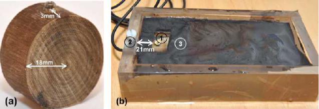

H. H. MUHAMMED, S. V. V. N. KOTHAPALLI

571

sensitive to the amount of bone (rabbit femur was used)

in contact with a cylindr ical titanium dental implant. The

transducer used in this study had a central frequency of

10 MHz to allow for distinguishing different echoes ori-

ginating from different i mplant inter faces. Furthermore, a

long-enough signal duration (25 times longer that used

by de Almeida et al. [7]) was used to retrieve more in-

formation from the implant and compute the indicator.

The new approach, proposed by this work, aims at

evaluating the stability of the dental implant screw in

bone and soft tissues. For this purpose, a proper phantom

is designed and used. Ultrasonic spectral analysis is uti-

lized to detect differences or changes in the shape of the

curve of the power spectrum of the ultrasonic echo-sig-

nals reflected from the phantom representing an implant

imbedded into a jawbone. An automatic statistical-mod-

eling method is developed and utilized to estimate (based

on analyzing the shape of ultrasonic power spectra) the

contact and the stiffness grade between the implant and

the jawbone.

However, in statistical modeling, two common prob-

lems are usually encountered: 1) Large number of va-

riables and few observations. 2) Explanatory and depen-

dent variables are collinear. These two problems can be

solved by, at first, preprocessing and normalizing the

data in an efficient way, then using a suitable Partial

Least Squares (PLS) algorithm to achieve the desired

results.

2. Materials and Methods

2.1. Phantom and Experimental Setup

A disc of fresh Oakwood was used to simulate a jawbone.

The speed of sound in Oakwood is about 3800 m/s [9],

which is close to the speed of sound in bone tissue,

which is about 3750 ± 250 m/s. The spongy microstruc-

ture of wood tissue is also similar to bone tissue making

it efficient to produce and use wood-based bone-implants

[10]. A metal screw was screwed into this wooden disc to

simulate an implant, as shown in Figure 1(a). This disc

was immersed into a pool filled with water and a

soft-tissue equivalent material; a black-colored mixture

composed of 4% graphite, 3% agar and 93% water [11].

An ultrasonic transducer was mounted at 21 mm distance

from the edge of the wooden disc as shown in Figure

1(b). The central or fundamental frequency of this single-

crystal piezoelectric ultrasonic transducer was 2 MHz,

and the frequency band was ranging from 1.8 MHz to 2.2

MHz.

A pulse generator with an amplifier was used to excite

the transducer to make it emit an ultrasonic pulse, then

receive the echo signal and transfer it through the am-

plifier to an oscilloscope. A power spectrum of the re-

ceived signal was generated by the oscilloscope by using

the fast Fourier transform (FFT). This spectrum was

transferred to a personal computer (PC), where it was

analyzed.

2.2. Dataset

A set of 30 power spectra was ac quir ed by the pulse-echo

ultrasound system described previously. Each power

spectrum corresponded to a certain contact level and a

certain stiffness grade between the metal screw and the

wooden disc. The contact level was measured in number-

of-turns when screwing the screw out or into the disc.

Initially, the screw was screwed in firmly in the wooden

disc. Thereafter, it was screwed out, a half turn each time,

to increase the gap between wood and screw gradually

until reaching 5 turns. Then it was screwed into the disc

again with a half turn each time until reaching the tight-

screw state again.

Finally, it was screwed out again exactly as before un-

til reaching 5 turn s. By this way, 10 different contact and

stiffness grades (linearly distributed between 0.5 and 5

turns) were simulated three times and the corresponding

power spectra were measured. Hence, the dataset availa-

ble for this work consisted of 30 power spectra and the

corresponding numbers of turns.

2.3. Methodology

1) Partial Least Squares (PLS): PLS is a multivariate

Figure 1. (a) Metal screw screwed into a wooden disc. (b) The experimental setup where the phantom, labeled with (1) and

presented i n Figure 1(a), is immersed into a pool filled with water and a soft-tissue equivalent material, labeled with (3). An

ultrasonic transducer, labeled with (2), is mounted 21 mm away from the edge of the phantom.

H. H. MUHAMMED, S. V. V. N. KOTHAPALLI

572

statistical framework which includes a wide class of me-

thods and is used for processing, interpreting and ana-

lyzing data, measurements and observations in a wide

range of fields and applications. An overview of PLS is

presented by Rosipal and Kramer [12].

The pioneering work of introducing PLS was mainly

done by Herman Wold in 1966 [13] and 1975 [14]. Since

then, PLS has received great attention in many research

fields. The basic principle of this method is to find and

use a small number of uncorrelated variables (known as

components or latent variables) to explain as much cova-

riance as possible between the two blocks of explanatory

X and dependent Y variables; where each column of the

X- and Y-matrices contains one variable.

At first, the X- and Y-variables are preprocessed to

make their distributions fairly symmetrical. The nth root

transformation (where n is a real number) can be used to

compress the dynamic range of these variables so that the

result of dividing the mean value by the standard devia-

tion (of this variable) will be around one. After that, a nor-

malization technique called whitening [15] is performed

to scale the data into zero-mean and unit-variance.

The general PLS model is described as follows:

XTPE YTQF=+=+

(1)

where X is an nxm matrix of predictors, Y is an nxp ma-

trix of responses, T is an nxl matrix of factors, P and Q

are mxl and p xl loading matrices (of w eight coefficients),

respectively, and matrices E and F contain error terms.

There exist a number of PLS algorithms to estimate

the factor and loading matrices T, P and Q. Most of these

algorithms estimate the linear regression between X and

Y as:

Y = XB + N (2)

where Y contains n cases and m dependent variables, X

contains n cases and p independent variables, B contains

pxm regression coefficients (reflecting the covariance

structure between Y and X), and N is a noise term of the

same size as Y.

2) Using PLS analysis: There exist many different

ways of performing PLS analysis. In this work the

non-linear iterative partial least squares algorithm (NIP-

ALS; [14]) is used. The first step of the NIPALS algo-

rithm is to create two matrices E = X and F = Y, where

the columns of X contain the measured ultrasonic power

spectra (which are our independent variables), while Y is

a vector contains the corresponding dependent variables

that are desired to be estimated.

The second step is to prepro cess and normalize both X

and Y. Each element of vector Y is transformed (by

choosing an appropriate power value) so that the result of

dividing its mean value by its standard deviation will be

around one. After that, whitening is applied to Y. Matrix

X is also whitened, but by employing two iterative nor-

malisation approaches, where a number of alternating

spectral-wise (denoted as Sw and performed row-wise in

matrix X) and band-wise (denoted as Bw and performed

column-wise in matrix X) whitening operations are per-

formed, as described in [16]. When performing Sw-whi-

tening, each spectrum (which corresponds to one row in

matrix X) is whitened, while each column of X (which

corresponds to one spectral band) is whitened when Bw-

whitening is performed. In the first iterative normalisa-

tion approach, a series of alternating Sw- and Bw-whi-

tening operations, beginning and ending with Sw-whi-

tening operations, were performed. On the other hand,

the second iterative approach started with a Bw-whiten-

ing operat i on and ended with a Sw-whitening opera t ion.

After that, the PLS algorithm starts and a series of

iterative operations are performed until convergence of

the result is achieved. At this point, the whole set of la-

tent variables are calculated, as explained by Abdi [17].

In order to avoid over modeling, the number of latent

variables to be included in the PLS model should be de-

termined. A rule of thumb is that each latent variable

used in the final model corresponds to five or six inde-

pendent observations in the training dataset. (Rhiel et al.

[18]).

By this way, an upper limit for how many latent va-

riables to include has been defined. The remaining ques-

tion is how many of these latent variables are enough to

include. A popular way to know that is by calculating the

relative error value which is zero when perfect prediction

is achieved. Otherwise, it is always a positive number.

The PLS model is improved as long as adding more la-

tent variables lowers the relative erro r value. The optimal

number of latent variables is found when the relative

error value begins to increase [17].

3) Cross validation: To evaluate the usefulness and ef-

ficiency of the PLS model, cross validation is necessary.

Leave-one-out cross validation is an efficient evaluation

method when few observations are available. Only one

pair of variables at a time is removed from the reference

dataset and the excluded dependent parameter (which is

desired to be estimated) is considered as unknown. The

rest of the data samples are considered as a training da-

taset and the excluded measured spectrum is fed into the

trained model to estimate the excluded dependent para-

meter.

The estimated parameter values are finally compared

to the real values, to evaluate the performance of the PLS

model. Both of the relative error and the coefficient of

determination R2 can be used as evaluation measure.

3. Experimental Results

The gap between the jawbone and the dental implant may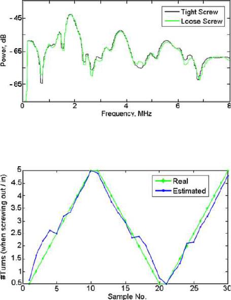

H. H. MUHAMMED, S. V. V. N. KOTHAPALLI

573

vary between zero and 0.1 mm, which is the initial gap

size when inserting a screw-type dental implant [19]. The

gap-size variation corresponds to a variation of the con-

tact and the stiffness grade between the implant and the

jawbone. However, what is more interesting and impor-

tant to know is if the osseointegration process is com-

plete or not, and if this process is progressing towards

obtaining a better intimate contact, between the bone and

the implant, or not. An efficient way to simulate varying

grades of osseointegration is to use the experimental se-

tup and the phantom described previously.

The nonlinear propagation of the ultrasonic waves

through the wooden disc, the metal screw and the wa-

ter-filled gap between them will gradually deform the

shape of the waves. Therefore, in addition to the effect of

Fourier transforming the time-signal received by the

transducer, higher harmonic frequencies (defined as in-

teger multiples of the fundamental frequency of the ul-

trasonic transducer) appear in the power spectrum. The

frequency of the peak of the first harmonic was shifted

from 2 MHz down to 1.92 MHz. The second harmonic

peak was at around 3.84 MHz, the third one was at

around 5.76 MHz and so on, as shown in Figure 2. Low

pass filtering was used to suppress the noise and get

smoother spectra.

It is essential to ensure the repeatability of the experi-

ments to validate the capability of an ultrasonic mea-

surement system. Therefore, the experiments were re-

peated using different initial conditions and the measured

power spectra were compared. The resulting standard

deviations , when comparing spectra correspo nding to the

same contact level, were mainly limited to 1%.

Figure 2 shows a comparison between two power

spectra; one corresponds to a tight screw and the other

one corresponds to a loose screw. It is possible to ob-

serve differences between these spectra, at the higher

harmonics. These differences are automatically utilized

by the PLS algorithm to be able to estimate the corres-

ponding stiffness grade which is measured in num-

ber-of-turns when screwing the metal screw out or into

the wooden disc. Before applying the PLS algorithm, the

power spectra were pr eprocessed according to the guide-

lines m e nt ioned previously.

Figure 3 presents a comparison between real and es-

timated stiffness grades (measured in number-of-turns),

with a coefficient of determination R2 of 96.4% and a

mean absolute error of ±0.23 turns.

4. Discussion and Conclusions

Although the obtained results indicate the usefulness and

efficiency of the used approach, the transducer was at-

tached to the phantom at approximately the same posi-

tion, angle and direction during the whole experiment.

Figure 2. A comparison between two power spectra; a

power spectrum of a tight screw and another one of a loose

screw.

Figure 3. A comparison between real and estimated num-

ber-of-tums when screwing the screw out, then in, then out

again. Various number-of-turns correspond to various stiff-

ness grades be tween the screw and wood.

Minor changes occurred when trying to screw in or out

the screw. The spectral measurements will change con-

siderably when measuring at different parts of the phan-

tom and from different directions or angles. However, it

is possible to normalize these spectra and make them

useable, since the method proposed and used in this work

doesn’t rely on comparing amplitudes of one or several

peaks found at certain frequency intervals. The new me-

thod makes instead use of the shape of the whole spec-

trum which makes it more efficient and practical so that

it can be used outside the laboratory without the need for

controlled measuring conditions. Furthermore, it is not

necessary to manually identify the most useful spectral

regions where most variations among the spectra are vis-

ible. The significance of the new method is that it is ob-

jective, non-invasive, fast, accurate, automatic and re-

producible.

REFERENCES

[1] P. I. Branemark, U. Breine, R. Adell, B. O. Hansson, J.

Lindstrom and A. Ohlsson, “Intra-Osseous Anchorage of

Dental Prostheses: I. Experimental Studies,” Journal of

Plastic and Reconstructive Surgery and Hand Surgery,

Informa Healthcare, Vol. 3, No. 2, 1969, pp. 81-100.

H. H. MUHAMMED, S. V. V. N. KOTHAPALLI

574

[2] D. W. Fitting and L. Adler, “Ultrasonic Spectral Analysis

for Nondestructive Evaluation,” Plenu m Press, New York,

1981. http://dx.doi.org/10.1007/978-1-4613-3126-1

[3] S. F. Lin, L. C. Pan, S. Y. Lee, Y. H. Peng and T. C.

Hsiao, “Resonance Frequency Analysis for Osseoi ntegra-

tion in Four Surgical Conditions of Dental Implants,”

Proceedings of the 23rd Annual International Conference

of the IEEE Engineering in Medicine and Biology Society,

Vol. 3, 2001, pp. 2998-3001.

[4] R. L. C. Pan and S. H. Ying, “Mechanical Properties of

Bone-Implant Interface: An in Vitro Model for the Com-

parison of Stability Parameters Affecting Various Stages

during Osseointegration for Dental Implant,” IEMBS’04

26th Annual International Conference of the IEEE Engi-

neering in Medicine and Biology Society, Vol. 2, 2005, pp.

5050-5052.

[5] P. Valderrama, T. W. Oates, A. A. Jones, J. Simpson, J. D.

Schoolfield and D. L. Cochran, “Evaluation of Two Dif-

ferent Resonance Frequency Devices to Detect Implant

Stability: A Clinical Trial,” Journal of Periodontology,

American Academy of Periodontology, Vol. 78, No. 2,

2007, pp. 262-272.

http://dx.doi.org/10.1902/jop.2007.060143

[6] V. Pattijn, S. V. N. Jaecques, E. De Smet, L. Muraru, C.

Van Lierde, G. Van der Perre, I. Naert and J. V. Sloten,

“Resonance Frequency Analysis of Implants in the Gui-

nea Pig Model: Influence of Boundary Conditions and

Orientation of the Transducer,” Medical Engineering &

Physics, Vol. 29, No. 2, 2007, pp. 182-190.

http://dx.doi.org/10.1016/j.medengphy.2006.02.010

[7] M. S. De Almeida, C. D. Maciel and J. C. Pereira, “Pro-

posal for an Ultrasonic Tool to Monit or the Osseointegra-

tion of Dental Implants,” Sensors, Molecular Diversity

Preservation International, Vol. 7, No. 7, 2007, pp. 1224-

1237.

[8] V. Mathieu, F. Anagnostou, E. Soffer and G. Haiat, “Ul-

trasonic Evaluation of Dental Implant Biomechanical Sta-

bility: An in Vitro Study,” Ult rasound in Medicine & Bio-

logy, Vol. 37, No. 2, 2011, pp. 262-270.

http://dx.doi.org/10.1016/j.ultrasmedbio.2010.10.008

[9] A. Walker, “The Encyclopedia of Wood,” Quatro Pub-

lishing, London 2005, p. 192.

[10] A. Tampieri, S. Sprio, A. Rufini, I. G. Lesci and N. Ro-

veri, “From Wood to Bone: Multi-Step Process to Con-

vert Hierarchical Structures into Biomimetic Hydroxya-

patite Scaffolds for Bone Tissue Engineering,” Journal of

Materials Chemistry, Vol. 19, No. 28, 2009, pp. 4973-

4980. http://dx.doi.org/10.1039/b900333a

[11] E. L. Madse n, J. A. Zagzebski, R. A. Banjavie and R. E.

Jutila, “Tissue Mimicking Materials for Ultrasound Phan-

toms,” Medical Physics , Vol. 5, 1978, p. 391.

http://dx.doi.org/10.1118/1.594483

[12] R. Rosipal and N. Kramer, “Overview and Recent Ad-

vances in Partial Least Squares,” Subspace, Latent Struc-

ture and Feature Selection: Statistical and Optimization

Perspectives Workshop, SLSFS 2005; Revised Selected

Papers, Springer-Verlag Inc., New York, 2006, pp. 34-51.

http://dx.doi.org/10.1007/11752790_2

[13] H. Wold , “Nonlinear Estimation by Iterative Least Square s

Procedures,” In: F. N. David, Ed., Festschrift for J. Ney-

man, Wiley, New York, 1966, p. 411.

[14] H. Wold, “Path Models with Latent Variables: The NIP-

ALS Approach,” Quantitative Sociology: International

Perspectives on Mathematical and Statistical Modeling,

1975, pp. 307-357.

[15] Y. C. Eldar and A. V. Oppenheim, “MMSE Whitening

and Subspace Whitening,” IEEE Transactions on Infor-

mation Theory, Vol. 49, No. 7, 2003, pp. 1846-1851.

http://dx.doi.org/10.1109/TIT.2003.813507

[16] H. Hamid Muhammed, “Hyperspectral Crop Reflectance

Data for Characterising and Estimating Fungal Disease

Severity in Wheat,” Biosystems Engineeri n g, Vol. 9 1, No.

1, 2005, pp. 9-20.

http://dx.doi.org/10.1016/j.biosystemseng.2005.02.007

[17] H. Abdi, “Partial Least Square Regression,” Encyclopedia

for Research Methods for the Social Sciences, 2003.

[18] M. Rhiel, M. B. Cohen, D. W. Murhammer and M. A.

Arnold, “Nondestructive Near-Infrared Spec trosco pic Mea-

surement of Multiple Analytes in Undiluted Samples of

Serum-Based Cell Culture Media,” University Of Iowa,

2001.

[19] R. K. Schenk and D. Buser, “Osseointegration: A Reality,”

Periodontology, Vol. 17, No. 1, 1998, pp. 22-35.