Propagation Modelling Using Integral Equation Methods to Enable Co-existence and Address Physical Layer Security Issues in Cognitive Radio

doi:10.4236/ijcns.2011.43017

Paper Menu >>

Journal Menu >>

Int. J. Communications, Network and System Sciences, 2011, 4, 139-146

doi:10.4236/ijcns.2011.43017 Published Online March 2011 (http://www.SciRP.org/journal/ijcns)

Pr opagation Modelling Using Integral Equation Methods to

Enable Co-Existence and Address Physical Layer Security

Issues in Cognitive Radio

Eamonn O. Nuallain

Centre for Telecommun ications Value Chain Research, Trinity College Dublin, Dublin, Ireland

E-mail: [email protected]

Received October 14, 2010; revised November 6, 2010; accepted November 8, 2010

Abstract

In this paper it is envisaged that cognitive radios (CRs) consult a supporting network infrastructure for per-

mission to transmit. The network server either grants or rejects these requests by estimating, from the CRs

geo-location and antenna features, the likely impact its transmission would have on incumbents and other CR

devices. This decision would be based on a real-time radio environment map [1] which would be kept up to

date with readings from CRs, sensors and dynamic radio propagation prediction. By this means coexistence

with incumbents and other CRs can be satisfied. It is maintained here that integral-equation (IE)—based al-

gorithms are suitable candidates for the propagation engine given their ‘automatic’ nature and that they can

be implemented to give results arbitrarily close to the exact numerical solution. IE methods based on the Fast

Multipole Method are examined as a likely route to achieve the accuracy and speed necessary for real-time

propagation mapping. It is concluded that the results obtained using one of the most recent of these, the Field

Extrapolation Method (FEXM) [2], are promising for rural/suburban profiles and could serve to enable co-

existence, for example, in IEEE802.22 networks. It is also explained how dynamic propagation prediction

can address some fundamental security threats to CR networks.

Keywords: Cognitive Radio, Propagation Modeling, Integral Equations

1. Introduction

Cognitive Radio (CR) is a radio technology th at refers to

the ability of a radio device to sense/learn the communi-

cation parameters of its environment and adapt its trans-

missions accordingly. The ability of a radio device to do

this with sufficient sophistication and agility will enable

such devices to transmit in underutilized licensed bands

without affecting the communications of the licensee.

CR presents the radio community with brand new

challenges. Chief among these is the ability of these de-

vices to co-exist with the incumbent operators and other

CRs without causing harmful interference.

Real-time radio environment mapping offers a means

by which this problem can be resolved. ‘The Radio En-

vironment Map (REM) itself is an abstraction of real-

world radio scenarios; it characterizes the radio envi-

ronment of CRs in multiple domains, such as geographi-

cal features, regulation, policy, radio equipment capabil-

ity profile and radio frequency emissions’ [1]—in short it

is a multidimensional map of what is happening in the

radio environment in multiple domains. The information

needed to create the signal strength portion of this real-

time map would be generated by a radio-propagation pre-

diction algorithm and interpolated/corrected by signal-

strength readings which are relayed to the server by CR

devices and sensors.

The signal-strength portion of the REM server would

then essentially act as a set of ‘traffic lights’ that a CR

device would consult each time it wished to transmit.

The effects of the requested transmission could be im-

mediately computed based on the GPS position of the

CR and the intended recipient using the propagation pre-

dictor and a digital terrain database hosted on the REM.

On the basis of whether or not this transmission would

adversely affect incumbents or other CRs a decision

would be made by the server whether or not to grant

permission to transmit and what the appropriate power

limitations should be. This is an explicit solution to the

Hidden Node Problem.

140 E. O. NUALLAIN

To this end a highly accurate and robust propagation

predictor capable of operating in a dynamic environment

is needed.

2. Propagation Prediction

Propagation prediction over terrain has received scant

attention in the academic literature in recent years. This

contrasts sharply with the attention it received in the

eighties and early nineties with the widespread deploy-

ment of 2G cellular systems; the industry generally set-

tling for sub-optimal models such as that of Hata, Wal-

fisch-Igekami and simple Ray-Tracing combined with

basic diffraction models such as Knife-Edge Diffraction

with which to pl an t hei r net w orks.

The reasons for this were twofold: Firstly, highly ac-

curate models are unnecessary for 2G and 3G networks.

Except in circumstances where terrain topology would

make it obvious to an experienced engineer where not to

place transmitters, large-scale fading would be present

regardless of transmitter location and so there is little

need for its precise prediction. The impact of these

large-scale fades on service quality is borne by the user,

which for voice and SMS is largely tolerable if overall

coverage is good.

Secondly, more sophisticated models, such as those

based on IE methods, were at this time underdeveloped

and computationally too expensive.

Furthermore there is no need for dynamic propagation

prediction for these networks. Propagation prediction is,

in the main, a once-off process concerned with base sta-

tions only and is performed at the time of network roll-

out.

It is for these reasons that IE methods have largely

remained the subject of scattering prediction from small

and medium-sized objects despite offering inherent ad-

vantages over other methods in propagation prediction

over terrain.

These advantages are: Given that the IE formulation is

the exact solution to the coverage problem there is no

need to reduce the problem to a number of canonical

ones. All electromagnetic phenomena (reflection, dif-

fraction etc.) are encapsulated in a single formulation. In

this sense IE methods can be said to be “automatic”

—that is, they can b e directly applied to an arbitrary ter-

rain database without human intervention and without

pre- processing and so are suitable for addressing dy-

namic propagat i on prediction pr o bl ems.

It is generally envisaged that CR networks will largely

be land-based and operate over distances of less than a

few kilometres. It is well known that th e large-scale fad-

ing signal can vary in the order of tens of decibels over

much shorter distances at frequencies of a few hundred

megahertz and upwards. To set reliable power limitations

when granting permission to transmit it is thus necessary

to use a propagation model which predicts large-scale

fading which is an inherent feature of IE methods.

Because IE methods are based on the exact numerical

formulation of the propagation problem, more reliable

numerical error margins can be established.

The main drawback of IE methods has been their

computational cost. This has been overcome by theoreti-

cal developments and by advances in computer technol-

ogy to the point where coverage results within approx.

8dB of measurement results for circa. 10Km two-di-

mensional rural profiles have been obtained on a stan-

dard desktop at sub-second speeds [2].

The formulation of the problem to be solved as an IE

is intuitively more acceptable than a differential equation

formulation. This eases the route to understanding and

physically inspired development.

For these reasons it is proposed that IE-based algo-

rithms form the basis for the real-time mapping of the

radio environment for CR in order to provide the degree

of reliability necessary in decision making regarding

transmissions and, as we shall see presently, in address-

ing some fundamental Physical-Layer security issues.

3. Security

Physical Layer problems such as malfunctioning nodes

and intentional jamming can be addressed in the follow-

ing manner. Central to this discussion is the fact that the

PU signal is unique to each topology and extremely dif-

ficult to replicate ph ysically outside of the vicinity of the

primary transmitter. It is in effect a digital signature.

By comparison of collected RSS data from CR nodes

and sensors with the predicted PU signal strength identi-

fication of malfunctioning nodes and/or security threats is

enabled.

To illustrate this concept let us consider the scenario

of an intentional ja mming attack. From the outset the PU

signal strength map as a function of location has been

established using a propagation predictor initially de-

rived from its location, a digital terrain database and the

maximum radiated power which are obtained from the

licensing authority or ‘learned’ by the network. This map

will have been refined with readings from sensors and

CR devices. This is our “pre-established” PU signal

strength map. During operation it is then observed that a

significant number of nodes are reporting the presence of

a PU signal. We may then check if the reported PU sig-

nal strength values versus location deviate from the

pre-established signal strength versus location values of

the PU. If so then we have grounds for suspecting that an

intentional jamming attack or a primary receiver jam-

E. O. NUALLAIN

141

ming attack is taking place. The latter is a passive jam-

ming attack where a malicious entity has unsuspecting

devices outside of the coverage region of the PU direct

their transmissions to it, which itself is located within the

coverage region of the PU. The result is harmful inter-

ference to the PU especially in regions of low signal

strength. Grounds for suspecting a jamming attack are

reinforced if the PU signal is reported to be present in a

locality to the contraindication of nodes which are at

other locations within the coverage region of the PU. The

region of highest “PU” signal strength will indicate the

location of the of fe n di n g device.

Dealing with malfunctioning nodes would be per-

formed in a similar manner, made simpler however, by

there being almost always nodes present to contraindi-

cate its readings which may not be the case with an in-

tentional jamming attack.

4. Integral Equation Methods

The Field Extrapolation Method (FEXM) is proposed

here as the basis for the propagation functionality of the

REM server described above—that is the core propaga-

tion engine.

In 1991 Prof. J. B. Andersen et al. published the first

paper on IE-based coverage prediction for terrain [3]. In

it they modelled the terrain profiles they examined as

two-dimensional perfect magnetic conductors. The re-

sults they obtained were compared with measurements

and results gi v e n by the Hata m odel .

It was clear that the results given by the unmodified IE

method were superior to those given by the Hata model

in terms of standard deviation from measured results and

that it predicted the large-scale fading signal very well.

However the computational complexity of the problem

was prohibitive being of the order where N is

sub-wavelength in dimension.





This prompted efforts to reduce the computational

complexity of the problem to enable the timely genera-

tion of results with a minimal compromise in accuracy.

According to Peterson [4] the Fast Multip le Method [5]

or variations thereof, “appear to offer the most efficient

possibilities yet proposed for the accurate numerical

analysis of electrically large geometries where N may be

far greater than 104”.

The evolution of the FEXM from the Fast Multipole

Method is traced here via other published methods which

will provide a means for critical analysis and hopefully

provide the reader with clues on how it may be further

enhanced – perhap s in conju n c t i on wit h ot her methods.

4.1. The Electric Field Integral Equation

The problem is treated as two-dimensional

TM , the

surface is taken to be a perfect electrical conductor (PEC)

and forward scattering is assumed—th at is all radiation is

taken to propagate away from the transmitter. These two

assumptions are justifiable for the case of grazing inci-

dence transmitter radiation which is predominantly the

case for the terrain profile examined here. All are sim-

plifying and not limiting assumptions.

The surface is impinged by a monochromatic

polarized cylindrical wave of wave number



emanat-

ing from an infinite, unit current carrying wire of negli-

gible cross-section, placed a distance above and trans-

verse to the terrain profile. A time variation of



assumed and suppressed.

An electric current J is induced on the surface, which

satisfies the Electric Field Integral Equation (EFIE):

 



EJH









ds



(1)

r and r



are vectors whose end-points are respectively

the scattering and receiving points

S. is the

source electric field incident on the surface at the point

given by .

()Er



is the wave impedance of the medium through

which the radiation propagates and



is a zero order

Hankel function of the second kind which is the Green’s

function for the problem. The surface is discretized into

N equal sized sampling intervals of length



with

centre-points indicated by the vectors i and r

r de-

pending on whether they are scattering or receiving in-

tervals respectively. Using the Method of Moments with

unit pulse basis functions and Dirac-delta weighting

functions we get the following matrix relation:

EZJ



(2)

where:







(2)

2 1.781

1ln

ZsH

Zs je



 

 









 





 









E and J are column vectors of length N. Z, known as

the impedance matrix, is and symmetric. The

elements in the strictly lower triangle of Z correspond to

forward-scattering and those in the strictly upper triangle

to back-scattering. The diagonal elements correspond to

the self-interaction of the sampling intervals. On the as-

sumption of forward scattering, which is equivalent to

setting the strictly upper triangu lar elements of E to zero,

J is determined by forward substitution:

NN

142

E. O. NUALLAIN

1 for 1,,

ijji

EJZ i







 (3)

The order of complexity of determining J is





ON .

The total field at points above the surface is th en the sum

of the field from the source and the field scattered by the

surface.

The surface is divided into groups each containing M

sampling intervals. There are th en NM such groups.

A point of note, the importance of which will become

apparent later, is that this equation converges and gives

almost identical results if the Hankel function is replaced

with its far-field approximation. Why this is so is not

clear but it is a very useful observation given that the

far-field form is much easier to manipulate algebraically.

4.2. The Fast Multipole Method

The N integration intervals on the surface are grouped

such that each group comprises M integration intervals.

The number of groups is then NM. Letting l and

l denote groups with cen tre po ints l an d l' respectively.

The impedance matrix may then be written:

G

 

BAB (4)

where:



,ll

jn m

nmn mll

all He













 (5a)

and



jjll

bjl e



 



  (5b)



 is the angle ll





 makes with the horizontal

and similarly for



.

Then:



l jllilii

lll iG

EbabJ









 



 s



 (6)

where and



1,, N



The complexity of this equation can be substantially

reduced if





can be diag onal i sed.

To this end we substitute the definitions for a and b

given in (5) so that this equation becomes:



ll il

llm jl

jm njn

mn llm il

He e





 

 









 













(7)

The inner summation is a convolution of two DFTs

and hence can be expressed as a product of two functions

if their DFTs are known. Th e DFT of





does

not ex ist since



Hx as . However we can truncate

the inner summation since it converges.

n

Via the identity:



cos

lj lj

lj jjm

mlj





















 











we can write:





ijl jllil















(8)

where:



cos

ij ij

Pjp

ll ll

aHe





 

























Now using Equat i on (8) in Equati o n (6) we have:



 



01,

l jllilii

iil iG

EbabJ













 











(9)

Replacing the outer integral with a Q-point summation

gives:



 



11,

ljllili i

qiiliG

EbabJ









 









(10)

This is the Fast Multipole Method (FMM) formulation

for the above described problem.

4.3. The Fast Far-Field Approximation

The Fast Far-Field Approximation (FAFFA) [6] can be

obtained from the FMM in the following way [7]:







 diverges as This does not occur if

we use the far-field approximation of the Hankel func-

tion which , as noted previously, does not affect the con-

vergence of the integral:

P



(2) 2

02jx

Hx e















(11)

This allows one to write:



sin 2

ll Pjp

ll pP

ll ll

aee





 













































;

sin 2

ll ll

 



















(12)

E. O. NUALLAIN

143

where ()





is the Dirac-delta function.

Hence:



sin 2

ij ll

l jllil

bbd







 



 

























(13)

Via L’Hopital’s Rule we get:





02ll

ijl jllilll

Heb







 



 (14)

The discrete form of the EFIE is separated into its near

and far-fiel d regions giving:





cos

illl il

illll j

IjGFF

ji j

jG NF

jeeJ

HJs











































(15)

where and

F denote the near and far-field

components of the scattered field respectively. In like

manner with the FMM, the summations may be viewed

as aggregation (at the scattering group l), translation

(between groups) and disaggregation (at the ‘receiving’

group l) stages in the order in which they are given

above. This is the Fast Far-Field Approximation. Com-

putational speed up is achieved since the result of the

disaggregation stage can be stored and reused.

G

4.4. The Tabulated Interaction Method

With the Tabulated Interaction Method [8] the integra-

tion intervals in a group are taken to be collinear and the

aggregation and disaggregation stages referred to in Lu

and Chew’s pape r [6 ] are pe rfo rmed fo r a r ang e of angl es

of incidence and reflection, lll j







and ll il







respectively, creating a lookup table which is then used

in performing the overall summation.

Using the approximation:

 





ilPlanei llil

JEJ







(16)

where ,



lanei llil

 

 is the surface current induced

at the point denoted by i



as a result of a unit ampli-

tude plane wave incident on the surface at an angle of

ll il



.

Then:



cos

ll jlll il

jllll j

GG j

lll

GFF

Planei llil

jij

jNF

EHeE

JH s



 

 































(17)

The inner summation (or disaggregation stage) having

been pre-computed can be accessed via a look-up table

thereby speeding up the solving process. Equation (14)

can be written more accurately as:











00ijlll jllilll

HHbb





 

 (18)

It is also noted that because of the nature of the prob-

lem—land-based transmission—the angles lll j







and

ll il







will generally be small—especially in the re-

gion near the observation point .

Then from Equations (17) and (18), making no dis-

tinction between the groups in the near and far-field, we

get the following approximation:



 



ll il

GG j

Illl

GjG

jij

EHeJ

JH s



































(19)

4.5. The Field Extrapolation Method

The TIM has shown that interactions between groups

may be considered as being due to plane- waves. Where

the groups are approximated as being collinear then it

follows that the surface current may be approximated as

being constant amplitude sinusoids. This a-priori as-

sumption of the form of the induced surface current over

a group can be used to circumvent the aggregation and

disaggregation stages of the FAFFA and the creation of a

look-up table in the TIM. The resulting algorithm is very

simple, very fast, has negligible memory requirements

and yields results of similar accuracy to the aforemen-

tioned.

It has been shown how the algorithm has its concep-

tual roots in all three of the above.

These are:

1) The fundamental concept of effectively grouping

integration intervals into equal sized regions has its ori-

gin in the FMM.

2) The concept of summing phase-shifted values of the

surface current at the group centre during “aggregation”

and performing the reverse procedure at the “disaggrega-

tion” stage has its roots in the FMM and the FAFFA.

3) The concept that group-group interactions can be

treated as being due to plane wave interactions has its

144 E. O. NUALLAIN

roots in the TIM.

All three of these concepts form the basis for the

FEXM. What follows is a heuristic derivation of the

FEXM starting with the FAFFA where the contributions

of the above concepts become clear.

From Equation (19), but treating near-field interac-

tions as though they are due to far-fields except at the

receiving group we get:



cos

ll illl il

illll j

GG j

IiG

ieJ





























(20)

This equation in itself does not converge to give the

correct solution. This is because the near-field interac-

tions have not been treated as such and so the above ap-

proximation is too crude. The near-field interactions are

those which have the greater bearing on convergence.

This corresponds to the disagg rega tion stage in th e above

equation. Because the angle ll il



 and lll j







will generally be small an d the aggregation phase can b e

combined with the translation phase with comparatively

little loss in accuracy, we get:



ll ll ilil

ll il

GG jj

GjG

GG j

ll j

GjG

EeeJ

HeJs

 













 



























(21)

The process of disaggregation is performed by the

phase shifting operator . It is now proposed that

this sensitive process is p erformed in both amplitude and

phase. This is achieved using the Green’s function for

the problem, namely the Hankel function.





The resulting equation is then:





Ijllij

GjG

EHHJ















  (22)

As was shown in the TIM, the surface current can be

modelled as having been induced by a plane wave. If

furthermore we assume that the amplitude of this current

is approximately constant over a group then we can

write:





cos

ji l

Illll

EHJ



























(23)

If, as in the case of the TIM, groups can be considered

to be flat the inner summation will be a constant where

the phase shift l



 is incorporated into the current

phasor. This latter approximation is reasonable since we

are not interested in small-scale fading. Hence:





Illl

EHJ







l









 (24)

where



0il

















(25)

This is a somewhat different result for K to that ob-

tained in [2] but the absolute value is similar. The phase

is arbitrary and can be absorbed into the current phasor

without any appreciable difference in the result for field

coverage at points t above the surface which, by similar

analysis is:

 





tt ltl

EE HJ

 









 

 (26)

From the above analysis it can be seen that the FEXM

achieves its accuracy by using the Green’s function as

the operator for disaggregation and its speed by virtue of

a-priori assumption of the form of the surface current

over a group. In this way the need to perform computa-

tionally expensive group-specific disaggregation or the

creation of look-up tables is obviated. The algorithm is

simple, lends itself easily to application on a digital ter-

rain database and like the EFIE this algorithm is paral-

lelizable.

5. Results

The following results were introduced in [9] and, it is

hoped, will serve to illustrate the preceding discussion.

The FEXM is applied at 435 MHz to a 7.85 Km semi-

rural terrain profile in Hadsund, Northern Denmark

shown in Figure 1. In Figure 2, a comparative plot of

results given by the FEXM, EFIE and measurements is

given. The transmitter is at an elevation of 16.4 m. All

measurements and computational results are taken at 2.4

m above the surface. All computations are performed on

a 2.2 GHz Pentium 4 processor. 10 m group sizes are

used to provide as accurate as possible a comparison

with measurements (which were taken every 10 m). The

execution time is 1.35 sec yielding a circa. 7.5 dB stan-

dard deviation with respect to measurements. Much lar-

ger group sizes can be used for these types of profiles

without greatly compromising accuracy. The execution

time using 50 m group sizes is 0.07 sec.

In Figure 3, the transmitter is placed 1m above the

surface, mimicking a CR, at x = 5 Km. The effect of the

transmission is plotted against location. The execution

times are as above.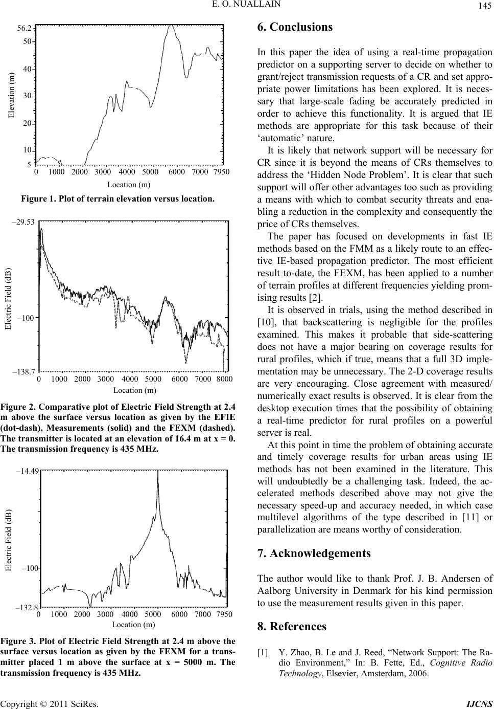

E. O. NUALLAIN

145

Location (m)

Elevation (m)

56.2

1000

2000

3000

4000

5000

6000

7000795

Figure 1. Plot of terrain elevation versus location.

Location (m)

Electric Field (dB)

–

29.53

1000

2000

3000

4000

5000

6000

7000 8000

–

100

–

138.7

Figure 2. Comparative plot of Electric Field Strength at 2.4

m above the surface versus location as given by the EFIE

(dot-dash), Measurements (solid) and the FEXM (dashed).

The transmitter is located at an elevation of 16.4 m at x = 0.

The transmission frequency is 435 MHz.

Location (m)

Electric Field (dB)

–

14.49

1000

2000

3000

4000

5000

6000

7000795

–

100

–

132.8

Figure 3. Plot of Electric Field Strength at 2.4 m above the

surface versus location as given by the FEXM for a trans-

mitter placed 1 m above the surface at x = 5000 m. The

transmission frequency is 435 MHz.

6. Conclusions

In this paper the idea of using a real-time propagation

predictor on a supporting server to decide on whether to

grant/reject transmission requests of a CR and set appro-

priate power limitations has been explored. It is neces-

sary that large-scale fading be accurately predicted in

order to achieve this functionality. It is argued that IE

methods are appropriate for this task because of their

‘automatic’ nature.

It is likely that network support will be necessary for

CR since it is beyond the means of CRs themselves to

address the ‘Hidden Node Problem’. It is clear that such

support will offer other advantages too such as providing

a means with which to combat security threats and ena-

bling a reduction in th e complexity and consequently th e

price of CRs themselves.

The paper has focused on developments in fast IE

methods based on the FMM as a likely route to an effec-

tive IE-based propagation predictor. The most efficient

result to-date, the FEXM, has been applied to a number

of terrain profiles at different frequencies yielding prom-

ising results [2].

It is observed in trials, using the method described in

[10], that backscattering is negligible for the profiles

examined. This makes it probable that side-scattering

does not have a major bearing on coverage results for

rural profiles, which if true, means that a full 3D imple-

mentation may be unnecessary. The 2-D coverage results

are very encouraging. Close agreement with measured/

numerically exact results is observed . It is clear from the

desktop execution times that the possibility of obtaining

a real-time predictor for rural profiles on a powerful

server is real.

At this point in time the problem of obtaining accurate

and timely coverage results for urban areas using IE

methods has not been examined in the literature. This

will undoubtedly be a challenging task. Indeed, the ac-

celerated methods described above may not give the

necessary speed-up and accuracy needed, in which case

multilevel algorithms of the type described in [11] or

parallelization are means worthy of consideration.

7. Acknowledgements

The author would like to thank Prof. J. B. Andersen of

Aalborg University in Denmark for his kind permission

to use the measurement results giv en in this paper.

8. References

[1] Y. Zhao, B. Le and J. Reed, “Network Support: The Ra-

dio Environment,” In: B. Fette, Ed., Cognitive Radio

Technology, Elsevier, Amsterdam, 2006.

E. O. NUALLAIN

146

[2] E. O. Nuallain, “An Efficient IE-Based Propagation Mo-

del,” IEEE Transactions on Antennas and Propagation,

Vol. 53, No. 5, May 2005, pp. 1836-1841.

doi:10.1109/TAP.2005.846812

[3] J. T. Hviid, J. B. Andersen, J. Toftgard and J. Bojer,

“Terrain-Based Propagation Model for Rural Areas—An

Integral Equation Approach,” IEEE Transactions in An-

tennas and Propagation, Vol. 43, No. 1, January 1995, pp.

41-46. doi:10.1109/8.366349

[4] A. F. Peterson, S. L. Ray and R. Mittra, “Computational

Methods for Electromagnetics,” IEEE Press, New York,

1998, pp. 37-45.

[5] R. Coifman, V. Rokhlin and S. Wandzura, “The Fast

Multipole Method for the Wave Equation: A Pedestrian

Description,” IEEE Antennas and Propagation Magazine,

Vol. 35, No. 3, 1993, pp. 7-12. doi:10.1109/74.250128

[6] C. C. Lu and W. C. Chew, “Fast Far Field Approximation

for Calculating the RCS of Large Objects,” Microwave

and Optical Technology Letters, Vol. 8, No. 5, 1995, pp.

238-241. doi:10.1002/mop.4650080506

[7] C. Brennan, “Numerical Methods for the Efficient Com-

putation of Electromagnetic Scattering from a Class of

Large Scale Perfect Electrical Conductors,” Thesis, Trin-

ity College, Dublin, 1998.

[8] C. Brennan and P. Cullen, “Tabulated Interaction Method

for UHF Terrain Propagation Problems,” IEEE Transac-

tions on Antennas and Propagation, Vol. 46, No. 5, 1998,

pp. 738-739. doi:10.1109/8.668921

[9] E. O. Nuallain, “A Proposed Propagation-Based Method-

ology with Which to Address the Hidden Node Problem

and Security/Reliability Issues in Cognitive Radio,” In-

ternational Conference on Wireless Communications, Net-

working and Mobile Computing, Dalian, 12-14 October

2008, pp. 1-5.

[10] D. Holliday, L. DeRaad and G. St-Cyr, “Forward-Back-

ward: A New Method for Computing Low-Grazing Angle

Scattering,” IEEE Transactions on Antennas and Propa-

gation, Vol. 44. No. 5, 1996, pp. 722-729.

doi:10.1109/8.496263

[11] J. M. Song and W. C. Chew, “Multilevel Fast Multipole

Algorithm for Solving Combined Field Integral Equa-

tions of Electromagnetic Scattering,” Microwave and Op-

tical Technology Letters, Vol. 10, No 1, 1995, pp. 14-19.

doi:10.1002/mop.4650100107