TransCAD and GIS Technique for Estimating Traffic Demand and Its Application in Gaza City

doi:10.4236/ojce.2013.34029

Paper Menu >>

Journal Menu >>

Open Journal of Civil Engineering, 2013, 3, 242-250

Published Online December 2013 (http://www.scirp.org/journal/ojce)

http://dx.doi.org/10.4236/ojce.2013.34029

Open Access OJCE

TransCAD and GIS Technique for Estimating Traffic

Demand and Its Application in Gaza City

Essam Almasri, Mohammed Al-Jazzar

Department of Civil Engineering, Islamic University of Gaza, Gaza, Palestine

Email: [email protected]

Received September 11, 2013; revised October 11, 2013; accepted October 18, 2013

Attribution License, which permits unrestricted use, distribution, and reproduction in any medium, provided the original work is

properly cited.

ABSTRACT

In the early nineties of the last century, the transportatio n system in Gaza Strip was born and new infrastructure projects,

especially road networks, were constructed. However, the construction lacked efficient application of a transportation

planning process. Transportation planning relies on traffic demand forecasting process. The conventional process is

impeded by extensive amount of socioeconomic data. One of the most widely-used models which mitigate this problem

is the TransCAD Model. This model is rarely used in Gaza Strip for traffic demand forecasting, and most of the prac-

tices depend mainly on a constant growth rate of traffic. Therefore, the main objective of this research is to apply this

model in Gaza City for traffic estimation. This model estimates the origin-destination matrix based on traffic count. The

traffic count was carried out at 36 intersections distributed around Gaza City. The results of traffic flow estimation ob-

tained from TransCAD are assigned to the Gaza maps using the GIS techniques for spatial analysis. It is shown that the

most congested area at present is the middle of the city especially at Aljala-Omer Almokhtar intersection. Therefore,

improvement scenarios of this area should be carried out. The results of calibration of traffic flow estimation show that

the differences between the estimated and the actual flows were less than 10%. In addition, network evaluation results

show that the network is expected to be more congested in 2015. This work can be used by transportation planners for

testing any network improvement scenarios and for studying their network performance.

Keywords: Transportation Planning; Traffic Demand Forecasting; Origin-Destination Estimation; Gaza; GIS

1. Introduction

Gaza Strip is situated at the southern part of the Palestin-

ian Territories. As shown in Figure 1, it includes five

governorates namely, Rafah, Khan-Younis, Middle, Gaza

and North Governorates [1]. The area of Gaza Strip is

about 365 k m2. It is a narrow coastal strip of land with a

length of 40 km along the Mediterranean Sea in the

Northwest di rection. It has 58 km borders with An-Naqa v

Desert to the East and South and 12 km with Egypt to the

Southwest. It takes its name from its main city Gaza [2].

According to the census conducted by the Palestinian

Central Bureau of Statistics (PCBS), the total number of

population of Gaza Strip at mid 2011 was 1.59 millions.

Gaza is the most densely populated governorate in Gaza

Strip with a density of 0.75 inhabitants/hectare. The area

of Gaza City is 7259.3 hectares and the number of popu-

lation at mid 2011 is 552,0 00 [3].

Gaza Strip transportation system is limited by small

and poorly developed road network. Before 1967, it had

a single railway line running from North to South of

Gaza Strip along its centre. However, currently it disap-

pears and little trackage remains. There is only a small

port which is limited to fishermen. Gaza International

Airport was opened in November 1998; however, it was

closed in October 2000. After the arrival of the Palestin-

ian National Authority from Diasporas in the early nine-

ties of the last century, the transportation system in Gaza

Strip was born and a dramatic and unprecedented in-

crease in the possession of the vehicles was observed. In

consequence of that, new infrastructure projects, espe-

cially road networks, were constructed. However, the

construction lacked efficient application of a transporta-

tion planning process. This led to deficiency in adopting

the suitable transport policies to mitigate the transporta-

tion problems resulting from urbanization and rapid in-

crease of population [4].

Transportation planning relies on travel demand fore-

E. ALMASRI, M. AL-JAZZAR 243

Figure 1. Governorates of Gaza Strip [1].

casting which involves prediction of the number of vehi-

cles or travellers that will use a particular transportation

facility in future. Since 1950’s, many travel demand

forecasting processes were developed, including conven-

tional four-stage travel demand forecasting process. This

process begins with collection of extensive data on land

use, socioeconomic, demographic, and network charac-

teristics [5]. The four steps of the process are sequenced

as trip generation, trip distribution, mode choice, and

traffic assignment. Trip generation determines the num-

ber of trips starting or ending at an area (zone) within a

given time such as per day or per hour. It is based on

determining a relationship between trip making and land

uses, household demographics, and other socioeconomic

factors. Trip distribution is the process by which the

planner calculates the pattern of trips between the zones.

It describes the number or proportion of trips from an

origin zone spread amongst all destination zones. Mode

choice computes the patterns of trips between origin and

destination zones that use a particular transportation

mode. Traffic assignment determines the volume of

travel for each individual movement at intersections of

the transportation network [6].

From the time when the convention al four-stage travel

demand forecasting was developed, a number of highly

critical reviews to the model have been seen. In response

to criticisms, improvements have been made on the four-

stage modeling approach and new modeling approaches

have come out [7]. According to [7], few of the devel-

oped models have already been tried in cities of devel-

oping countries. An example of work is shown in [8] in

which different Work-Trip Mode-Choice Models for

South Africa were tested. A second example is shown in

[9] in which different trip generation models in develop-

ing countries were analyzed and calibrated. A third ex-

ample is shown in [10] in which two types of gravity

model for trip distribution in India were calibrated. A

fourth is [11] which is a transport study of Amman, Jor-

dan.

One of the criticisms of th e sequential four-step model

is the extensive amount of land use, socioeconomic, and

demographic data needed for the first step of trip genera-

tion. Because of that, many models have been developed

which skipped this step and started directly from step 2.

They estimate the origin-destination (O-D) matrix based

on traffic counts. Traffic counts are much easier to obtain

and are often already available for other traffic related

purposes. Therefore, many computer models have been

proposed and applied for O-D matrix estimation to inves-

tigate the relationship between traffic counts and O-D

matrix. One of the most widely-used models is the

TransCAD Model [12].

This model is rarely used in Gaza Strip for traffic de-

mand forecasting, and most of the practices depend

mainly on a constant growth rate of traffic. Therefore, the

main objective o f this research is to apply the Tran sCAD

model for traffic estimation. The results will be assigned

to the Gaza maps using the GIS techniques available in

TransCAD for spatial analysis to be used as guidelines

for transportation planner to determine the congested

locations in Gaza, and hence to help in developing poli-

cies for congestion mitigation .

2. Methodology

In order to achieve the objectives of this study the work

is divided into six phases. The first phase is data collec-

tion. The data includes network road characteristics and

traffic data for the base year. The traffic count was car-

ried out in 18/4/2010 by more than one hundred observ-

ers under the supervision of the researchers. The count

was conducted to from 7:00 am to 12:00 am to deter-

mine the exact network peak hour. It was done at 36 in-

tersections distributed around Gaza City as shown in

Figure 2.

Figure 2. Locations of traffic counts in Gaza City.

Open Access OJCE

E. ALMASRI, M. AL-JAZZAR

244

The second phase is network building and data enter-

ing. An aerial photo of Gaza was geo-referenced and

digitized using ArcGIS. The resulted ESRI shape file was

transferred into TransCAD and used as a background to

draw the network and the zones. Zoning system for Gaza

City was very essential for the O-D matrix estimation

and traffic assignment. For that purpose, the land use

characteristics of the City was studied.

The third phase is matrix estimation for the base year.

It is done using TransCAD Model which is based on

Nielsen’s Model [13], who independently developed it as

a procedure for TransCAD 2.1. The model has the ad-

vantages of handling counts as stochastic variables, as

well as working with any traffic assignment method.

Thus, it is appealing for use with the Stochastic User

Equilibrium Assignment method, as well as with User

Equilibrium Assignment. Nielsen’s model is an iterative

(or bi-level) process that switches back and forth be-

tween a traffic assignment stage and a matrix estimation

stage [14]. To use the O-D Matrix Estimation procedure,

the base O-D matrix and a geographic file of both area

and line laye rs are prepar ed. In line geographic file, each

link data should be input, and a network for the line layer

should be created. It should include all the relevant at-

tributes. In area geographic file, connectors of zones’

centroids must be created to connect line and area geo-

graphic layer. Because there is no available prior O-D

matrix, a unit matrix (each O-D pair has a value of 1)

was used as initial matrix. Based on traffic counts at the

intersections, the O-D matrix was estimated and vali-

dated. A base O-D matrix serves two purposes. The first

purpose is to set the dimensions for the output matrix.

The second purpose is to provide initial values for the

estimated O-D matrix.

The fourth phase is model calibration to ensure good

representation of the traffic network. The aim is to esti-

mate O-D matrix that should be as real as possible.

Model calibration was conducted by adjusting locations

of zones’ connectors, locations of zones’ centroids and

turn penalties. The observed traffic flow and the modeled

traffic flow at the intersections using the traffic assign-

ment should be close to each other. Traffic flow differ-

ence of 10% could be acceptable.

The fifth phase is future O-D matrix estimation. For

that purpose, it is recommended to use uniform growth

factor method by multiplying all O-D pairs by the same

amount as shown in Equation (1) [6]:

ijf ijppf

TTM (1)

where, ijf is trips for O-D pair ij in future year f; ijp

is trips for O-D pair ij in present year p; and

T T

expected growth in trips between year f and p.

When information about the expected growth in trips

produced in each zone is available, the singly constrained

growth factor method might be used ([6,15]). This is

performed by multiplying different growth factors to

different rows (or columns) in the O-D matrix. Accord-

ing to [6,16], the growth factors might be determined

based on land use or socioeconomic data. Because of

little amount of socioeconomic and land use data, fore-

casting in this research is simply based on uniform

growth factor method. The estimates of rate of growth in

vehicle ownership over the forecasting period are used to

develop the end product of passenger traffic trip matrix.

They are directly input to the modelling process as a

value by which existing base year vehicle trip matrices

are factored to develop future year trip matrices.

The sixth phase is network evaluation. TransCAD

model offers three network performance measures. The

first one is vehicles hours of travel which is the summa-

tion of travel time spent by all vehicles in the network.

The second one is the total vehicle kilometers travelled

which is the summation of the total distance travelled by

all the vehicles over the network in one hour. These two

measures can be used in different scenario evaluation and

comparison, where the best scenario should have the

lowest values. The third performance measure is volume

over capacity ratio which is a direct indication of the

network level of service.

3. Results and Analysis

This section presents the results obtained when applying

the methodology discussed in the previous section. It

includes five parts. The first one presents geometric and

traffic data. The second part concerns the network build-

ing. The third part discusses the obtained results of base

year O-D matrix estimation and model calibration, while

the fourth part discusses the results of future O-D matrix

estimation. The last part presents the results of network

evaluation.

3.1. Data

The geometric data collection focused on the main streets

and intersections which were involved in th e traffic count.

Figure 2 presents the intersectio ns’ names and locations.

Geometric data for some of the intersections are pre-

sented in Table 1 which are the intersections located

along Aljala Street. The first column is intersection serial

number. The second column shows the names of the in-

tersections while the third shows the names of the streets

intersecting Aljala Street. The next columns present the

number of lanes in each approach before arriving at each

intersection. It is noted that the lanes before arriving in-

tersections is less than at intersections because of either

widening of the intersections or using nearside lane for

parking between intersections. Table 2 presents the car-

riageway widths of the streets.

Open Access OJCE

E. ALMASRI, M. AL-JAZZAR

Open Access OJCE

245

Table 1. Geometric data for intersections located along Aljala Street.

Intersection Number of lanes

Before intersection At intersection

No. Name Aljala St. with… NB SB EB WB NB SB EB WB

25 El-Tiaran Jamal Abed Alnaser - 2 2 2 - 3 3 2

20 El-Saraya Omer Almokhtar st 2 2 2 2 3 3 3 3

13 Dabeet Alwehda 2 2 2 2 3 3 2 2

7 El-Ghifary Alababidy 2 2 2 2 3 3 3 3

4 1st st. 1st st. 2 2 2 2 3 3 3 3

3 Akher Aljala 3rd st. 2 2 2 2 2 2 2 2

Table 2. Carriageway widths of streets intersecting Aljala

Street.

No. Streets names Carriageway width (m)

1 Aljala Street 10

2 Jamal Abed Alnaser Street 8

3 Omer Almokhtar Street 10

4 Alwehda Street 6

5 Alababidy Street 9.5

6 The 1st Street 9

7 The 3rd Street 7

The traffic count at the 36 intersections was carried out

manually and simultaneously by 132 observers. At each

approach in each intersection, an observer stood and

counted vehicles that left the intersection and went left,

through or right. Figure 3 presents locations of the

counted intersections. The flows at the intersections are

shown in Figure 3 on GIS spatial map where the diame-

ter of the circle represents the summation of traffic flow

for all approaches at the intersection. Based on this rep-

resentation, it can be easily seen that the most congested

area is the middle of the city and that the intersections

and the streets in this area should be taken into consid-

eration.

Figure 4 presents graphically the values of total five-

hour traffic flow and the peak hour flow at the intersec-

tions. It is observed that Aljala-Omer Almokhtar inter-

section (Alsaraia) has the highest traffic flow. On the

other side, Alrashed-the third intersection (Almokhabarat)

has the lowest traffic flow. Network peak hour flow is

essential input in TransCAD to model the Gaza traffic

network. Based on the traffic count conducted to from

7:00 am to 12:00 am, the network peak hour was be-

tween 7:30 and 8:30 am.

3.2. Network Building

Network building in TransCAD is done by constructing

line geographic and area geographic layers. In line geo-

graphic layer, roads are represented by their centerlines.

For that purpose, an aerial photo of Gaza City was

geo-referenced and then the roads were digitized out of

the map by ArcGIS as shown in Figure 5. The process of

representing an image by a discrete set of its points is

known as the digitization process. The resulted ESRI

shape file was transferred into TransCAD. The geo-ref-

erenced ESRI shape file was then used as a background

to draw the network.

A zone area geographic layer is needed to complete

the traffic network modeling. Thirty four zones were

built in this layer. The resulting layer of zones and streets

is shown in Figure 6.

The selection of zonal boundaries was based on the

following criteria that were adopted in previous studies

such as [11,17]:

 The area of Central Business District (CBD) should

have relatively small zone sizes while larger zone

sizes are used for outside CBD. This is due to the

dense trip activities within CBD.

 The use of main roads as zone boundaries should be

avoided to facilitate the trip assigning for the zones

on or near the main roads.

 Each zone should have homogenous socio-economic

characteristics.

 The zoning process should take the Municipality dis-

trict’s boundaries into consideration.

3.3. Base Year Matrix Estimation and Model

Calibration

Based on the process of matrix estimation discussed in

the methodology section, the estimated O-D matrix for

base year 2010 is shown in Table 3. The number of

columns and rows is the number of zones. The zones in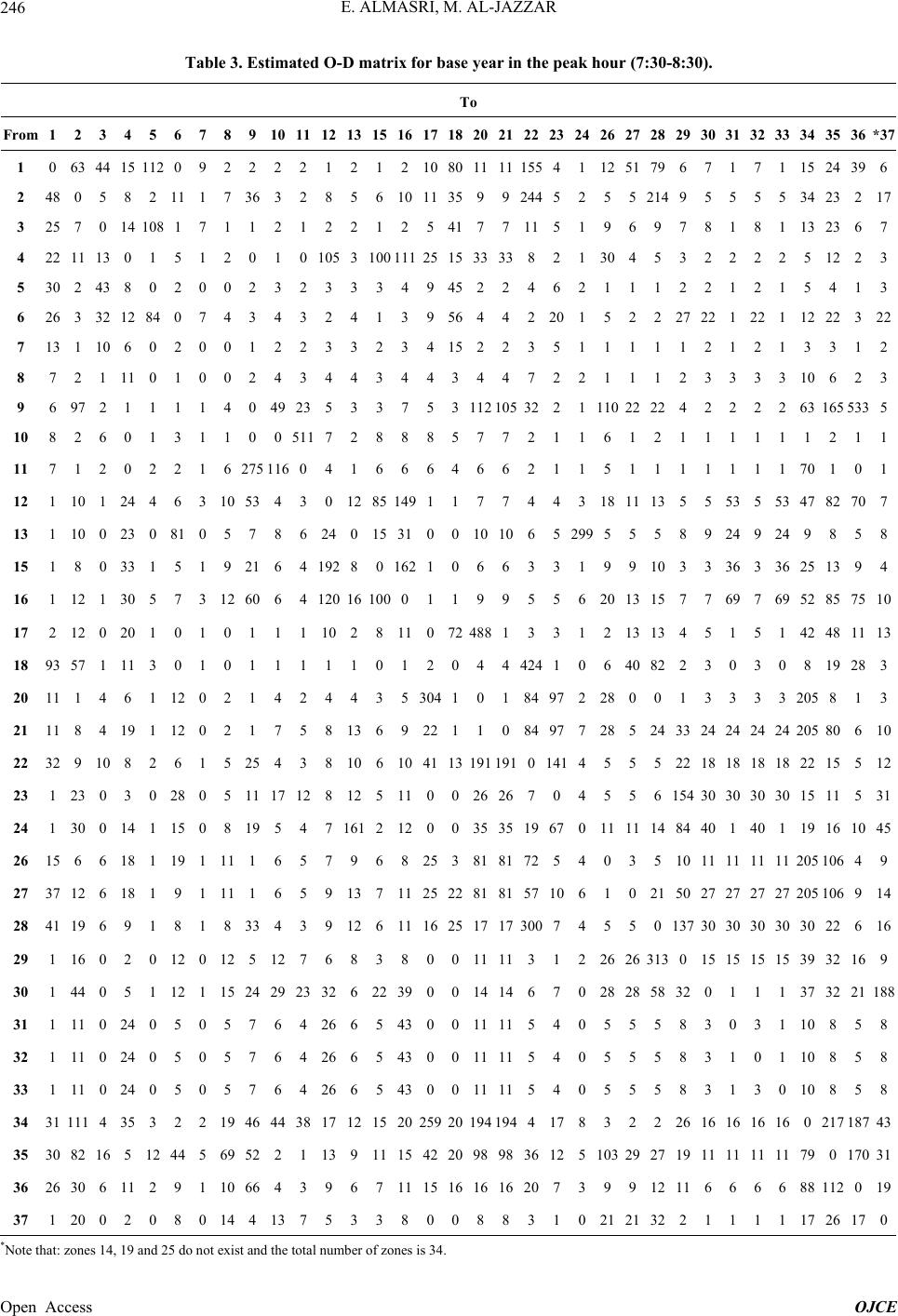

E. ALMASRI, M. AL-JAZZAR

246

Table 3. Estimated O-D matrix for base year in the peak hour (7:30-8:30).

From 1 2 3 4 5 6 7 89 10 11 12 1315161718202122232426272829 30 31 32 33 343536*37

1 0 63 44 15 112 0 9 22 2 2 1 21210801111155411251796 7 1 7 1 1524396

2 48 0 5 8 2 11 1 7 36 3 2 8 56 101135 9924452552149 5 5 5 5 3423217

3 25 7 0 14 108 1 7 11 2 1 2 212541 7711519697 8 1 8 1 132367

4 22 11 13 0 1 5 1 20 1 0 105 31001112515333382130 453 2 2 2 2 51223

5 30 2 43 8 0 2 0 02 3 2 3 334945 224621112 2 1 2 1 5413

6 26 3 32 12 84 0 7 43 4 3 2 413956 44220152227 22 1 22 1 1222322

7 13 1 10 6 0 2 0 01 2 2 3 323415 223511111 2 1 2 1 3312

8 7 2 1 11 0 1 0 02 4 3 4 43443447221112 3 3 3 3 10623

9 6 97 2 1 1 1 1 40 49 23 5 3375311210532 2111022224 2 2 2 2 631655335

10 8 2 6 0 1 3 1 10 0 511 7 28885772116121 1 1 1 1 1211

11 7 1 2 0 2 2 1 6275 116 0 4 16664662115111 1 1 1 1 70101

12 1 10 1 24 4 6 3 1053 4 3 0 1285149117744318 11135 5 53 5 53 4782707

13 1 10 0 23 0 81 0 57 8 6 24 015 310010 1065 299 5558 9 24 9 24 9858

15 1 8 0 33 1 5 1 9 21 6 4 192 80162106633199 10 3 3 36 3 36 2513 94

16 1 12 1 30 5 7 3 1260 6 4 120 16100 0119955620 13 157 7 69 7 69 52 857510

17 2 12 0 20 1 0 1 01 1 1 10 28 110 72488133121313 4 5 1 5 1 42481113

18 93 57 1 11 3 0 1 01 1 1 1 10120444241064082 2 3 0 3 0 819283

20 11 1 4 6 1 12 0 21 4 2 4 435304101 8497228 001 3 3 3 3 205813

21 11 8 4 19 1 12 0 21 7 5 8 1369221108497728524 33 24 24 24 24 20580610

22 32 9 10 8 2 6 1 5 25 4 3 8 10 61041131911910141455522 18 18 18 18 2215512

23 1 23 0 3 0 28 0 5 11 17 12 8 1251100 2626704556154 30 30 30 30 15115 31

24 1 30 0 14 1 15 0 819 5 4 7 161212003535196701111 1484 40 1 40 1 19161045

26 15 6 6 18 1 19 1 111 6 5 7 96825381 81 725403510 11 11 11 11 205106 49

27 37 12 6 18 1 9 1 111 6 5 9 13711 25 228181571061021 50 27 27 27 27 205106914

28 41 19 6 9 1 8 1 8 33 4 3 9 12 6111625171730074550137 30 30 30 30 30226 16

29 1 16 0 2 0 12 0 125 12 7 6 8380011113122626313 0 15 15 15 15 3932169

30 1 44 0 5 1 12 1 1524 29 23 32 62239 001414 67028285832 0 1 1 1 373221188

31 1 11 0 24 0 5 0 57 6 4 26 65 4300 11115405558 3 0 3 1 10858

32 1 11 0 24 0 5 0 57 6 4 26 65 4300 11115405558 3 1 0 1 10858

33 1 11 0 24 0 5 0 57 6 4 26 65 4300 11115405558 3 1 3 0 10858

34 31 111 4 35 3 2 2 1946 44 38 17 12 152025920194194417832226 16 16 16 16 021718743

35 30 82 16 5 12 44 5 6952 2 1 13 911154220989836125103 292719 11 11 11 11 790170 31

36 26 30 6 11 2 9 1 1066 4 3 9 67 1115161616207399 1211 6 6 6 6 88112019

37 1 20 0 2 0 8 0 144 13 7 5 3380088310 212132 2 1 1 1 1 1726170

*Note that: z ones 14, 19 and 25 do not exist and the total number of zones is 34.

Open Access OJCE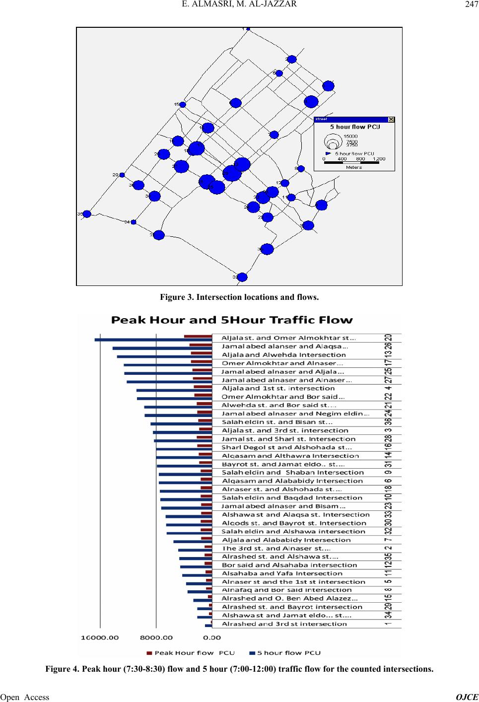

E. ALMASRI, M. AL-JAZZAR 247

Figure 3. Intersection locations and flows.

Figure 4. Peak hour (7:30-8:30) flow and 5 hour (7:00-12:00) traffic flow for the counted intersections.

Open Access OJCE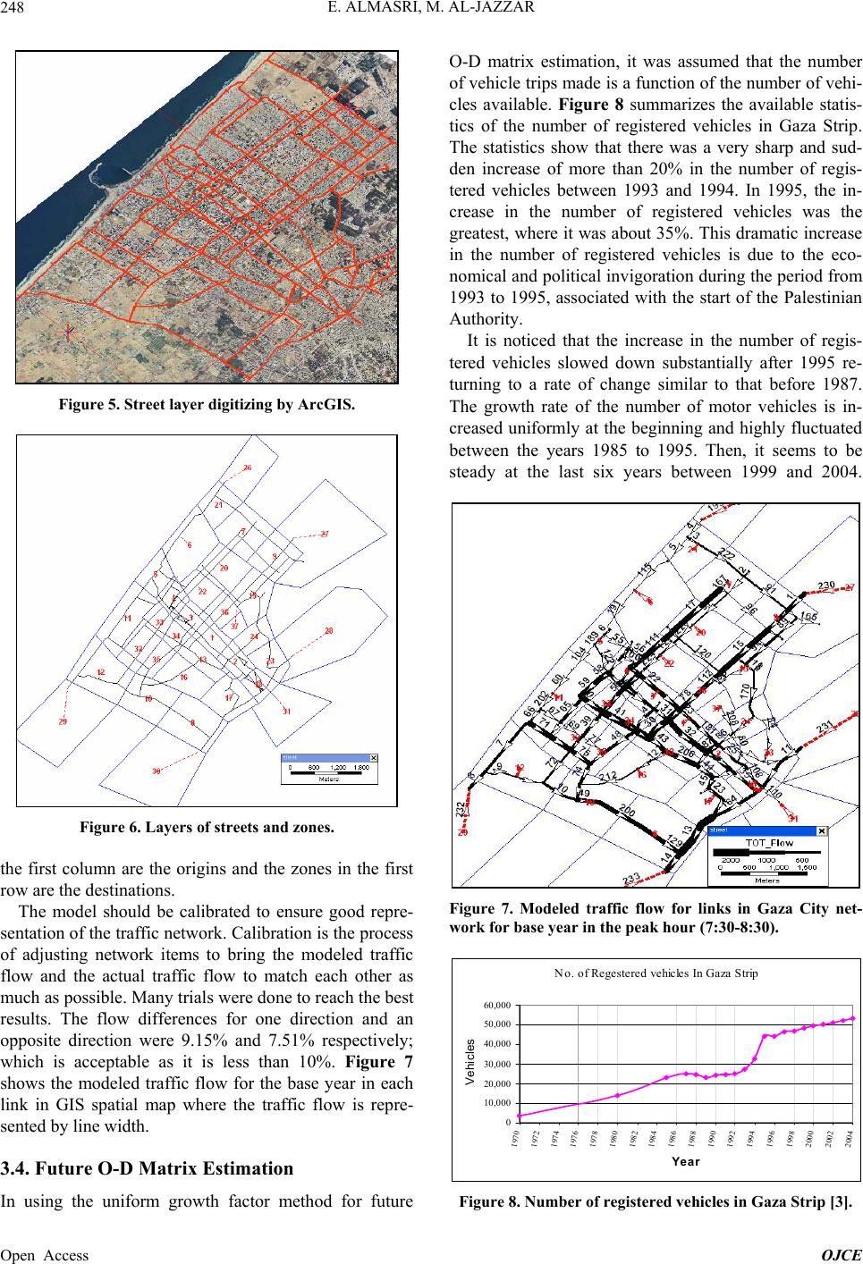

E. ALMASRI, M. AL-JAZZAR

Open Access OJCE

248

Figure 5. Street layer digitizing by ArcGIS.

Figure 6. Layers of streets and zones.

the first column are the origins and the zones in the first

row are the destinations.

The model should be calibrated to ensure good repre-

sentation of the traffic network. Calibratio n is the process

of adjusting network items to bring the modeled traffic

flow and the actual traffic flow to match each other as

much as possible. Many trials were done to reach the best

results. The flow differences for one direction and an

opposite direction were 9.15% and 7.51% respectively;

which is acceptable as it is less than 10%. Figure 7

shows the modeled traffic flow for the base year in each

link in GIS spatial map where the traffic flow is repre-

sented by line width.

3.4. Future O-D Matrix Estimation

In using the uniform growth factor method for future

O-D matrix estimation, it was assumed that the number

of vehicle trips made is a function of the number of vehi-

cles available. Figure 8 summarizes the available statis-

tics of the number of registered vehicles in Gaza Strip.

The statistics show that there was a very sharp and sud-

den increase of more than 20% in the number of regis-

tered vehicles between 1993 and 1994. In 1995, the in-

crease in the number of registered vehicles was the

greatest, where it was abou t 35%. This dramatic increase

in the number of registered vehicles is due to the eco-

nomical and political inv igoration during the period from

1993 to 1995, associated with the start of the Palestinian

Authority.

It is noticed that the increase in the number of regis-

tered vehicles slowed down substantially after 1995 re-

turning to a rate of change similar to that before 1987.

The growth rate of the number of motor vehicles is in-

creased uniformly at the beginning and highly fluctuated

between the years 1985 to 1995. Then, it seems to be

steady at the last six years between 1999 and 2004.

Figure 7. Modeled traffic flow for links in Gaza City net-

work for base year in the peak hour (7:30-8:30).

No. of Regestered vehicles In Gaza Strip

10,0 0 0

20,0 0 0

30,0 0 0

40,0 0 0

50,0 0 0

60,0 0 0

1970

1972

1974

1976

1978

1980

1982

1984

1986

1988

1990

1992

1994

1996

1998

2000

2002

2004

Year

Vehicles

Figure 8. Number of registered vehicles in Gaza Strip [3].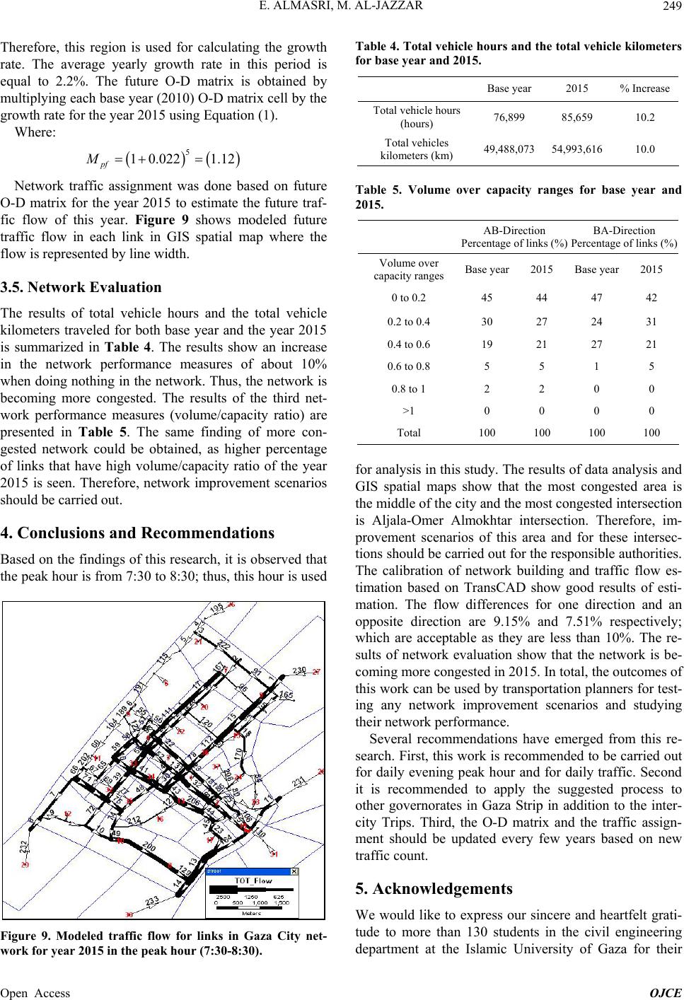

E. ALMASRI, M. AL-JAZZAR 249

Therefore, this region is used for calculating the growth

rate. The average yearly growth rate in this period is

equal to 2.2%. The future O-D matrix is obtained by

multiplying each base year (2010) O-D matrix cell by the

growth rate for the year 2015 using Equation (1).

Where:



1 0.0221.12

M 



Network traffic assignment was done based on future

O-D matrix for the year 2015 to estimate the future traf-

fic flow of this year. Figure 9 shows modeled future

traffic flow in each link in GIS spatial map where the

flow is represented by line width.

3.5. Network Evaluation

The results of total vehicle hours and the total vehicle

kilometers traveled for both base year and the year 2015

is summarized in Table 4. The results show an increase

in the network performance measures of about 10%

when doing nothing in the network. Thus, the network is

becoming more congested. The results of the third net-

work performance measures (volume/capacity ratio) are

presented in Table 5. The same finding of more con-

gested network could be obtained, as higher percentage

of links that have high volume/capacity ratio of the year

2015 is seen. Therefore, network improvement scenarios

should be carried out.

4. Conclusions and Recommendations

Based on the findings of this research, it is observed that

the peak hour is from 7:30 to 8:30; thus, this hour is used

Figure 9. Modeled traffic flow for links in Gaza City net-

work for year 2015 in the peak hour (7:30-8:30).

Table 4. Total vehicle hours and the total vehicle kilometers

for base year and 2015.

Base year 2015 % Increase

Total vehicle hours

(hours) 76,899 85,659 10.2

Total vehicles

kilometers (km) 49,488,073 54,993,616 10.0

Table 5. Volume over capacity ranges for base year and

2015.

AB-Direction

Percentage of links (%) BA-Direction

Percentage of links (%)

Volume over

capacity ranges Base year2015 Base year2015

0 to 0.2 45 44 47 42

0.2 to 0.4 30 27 24 31

0.4 to 0.6 19 21 27 21

0.6 to 0.8 5 5 1 5

0.8 to 1 2 2 0 0

>1 0 0 0 0

Total 100 100 100 100

for analysis in this study. The results of da ta analysis and

GIS spatial maps show that the most congested area is

the middle of the city and the most congested intersection

is Aljala-Omer Almokhtar intersection. Therefore, im-

provement scenarios of this area and for these intersec-

tions should be carried out for the responsible authorities.

The calibration of network building and traffic flow es-

timation based on TransCAD show good results of esti-

mation. The flow differences for one direction and an

opposite direction are 9.15% and 7.51% respectively;

which are acceptable as they are less than 10%. The re-

sults of network evaluation show that the network is be-

coming more congested in 2015. In total, the outcomes of

this work can be used by transportation planners for test-

ing any network improvement scenarios and studying

their network performance.

Several recommendations have emerged from this re-

search. First, this work is recommended to be carried out

for daily evening peak hour and for daily traffic. Second

it is recommended to apply the suggested process to

other governorates in Gaza Strip in addition to the inter-

city Trips. Third, the O-D matrix and the traffic assign-

ment should be updated every few years based on new

traffic count.

5. Acknowledgements

We would like to express our sincere and heartfelt grati-

tude to more than 130 students in the civil engineering

department at the Islamic University of Gaza for their

Open Access OJCE

E. ALMASRI, M. AL-JAZZAR

Open Access OJCE

250

help in collecting data.

REFERENCES

[1] Euro-Mediterranean Human Rights Network, 2013.

http://www.euromedrights.org/eng/

[2] E. Almasri, “Factors Affecting Travel Choice of Shared

Taxi versus Bus for Palestinian University Student Trips,”

International Review of Civil Engineering, Vol. 2, No. 1,

2011, pp. 35-45.

[3] Palestinian Central Bureau of Statistics, 2011.

http://www.pcbs.gov.ps/site/lang__en/1/default.aspx

[4] E. Almasri, “Improving Traffic Performance by Coordi-

nating Traffic Signals Using Transyt-7f Model—Eljalaa

Arterial Road in Gaza City as a Case Study,” Proceedings

of the 4th International Engineering Conference, Gaza,

15-16 October 2012.

[5] N. J. Garber and L. A. Hoel, “Traffic and Highway Engi-

neering,” 4th Edition, SI Cengage Learning, USA, 2010.

[6] C. A. O’Flaherty, “Traffic Planning & Engineering,” Ar-

nold, London, 1997, pp. 118-128.

[7] H. Bwire, “A Unified Framework for Selecting a Travel

Demand Forecasting Model for Developing Countries,”

Transportation Planning and Technology, Vol. 31, No. 3,

2008, pp. 347-368.

http://dx.doi.org/10.1080/03081060802087809

[8] P. R. Stopher and C. G Wilmot, “Work-Trip Mode Choice

Models for South Africa,” Transportation Engineering

Journal of ASCE, Vol. 105, No. TE6, 1979, pp. 595-608.

[9] K. Takyi, “Trip Generation Analysis in a Developing

Country Context,” Transportation Research Record, 1285,

pp. 9-21, 1990.

[10] V. T. Arasan, M. Wermuth and B. S. Srinivas, “Model-

ling of Stratified Urban Trip Distribution,” ASCE Journal

of Transportation Engineering, Vol. 122, No. 5, 1996, pp.

342-349.

http://dx.doi.org/10.1061/(ASCE)0733-947X(1996)122:5

(342)

[11] Dar Al Handasa, “the Greater Amman Urban Transport

Study,” Jordan, 1999.

[12] Caliper, “TransCAD Transportation Planning Software,”

2011. http://www.caliper.com/TCTravelDemand.htm.

[13] O. A. Nielsen, “A New Method for Estimating Trip Ma-

trices from Counts,” Institute of Roads, Traffic and Town

Planning, The Technical University of Denmark, 1993.

[14] Caliper Corporation, “TransCAD 4.5 Help for Planning,”

2002.

[15] J. D. D. Ortúzar and L. G. Willum, “Modeling Trans-

port,” John Wiley & Sons, LTD, England, 2001.

[16] K. Hamad and A. Faghri, “An Innovative Methodology

for Vehicular Demand Forecasting in Developing Coun-

tries,” TRB Annual Meeting, 2003.

[17] R. D. Douleh, “The Use Of Traffic Assignment Model-

ling Technique in Evaluating & Testing Transportation

Policies and Projects Nablus City: Case Study,” Master

Thesis, An-Najah National University, Nablus, 2000.