An Early Warning Model with Technical Indicators: The Case of Ise (Istanbul Stock Exchange)

doi:10.4236/ib.2013.54022

Paper Menu >>

Journal Menu >>

iBusiness, 2013, 5, 173-183

Published Online December 2013 (http://www.scirp.org/journal/ib)

http://dx.doi.org/10.4236/ib.2013.54022

Open Access IB

173

An Early Warning Model with Technical Indicators: The

Case of Ise (Istanbul Stock Exchange)

Kutluk Kagan Sumer

Department of Econometrics, Faculty of Economics, Istanbul University, Istanbul, Turkey.

Email: [email protected]

Received June 14th, 2011; revised July 12th, 2013; revised August 10th, 2013

which permits unrestricted use, distribution, and reproduction in any medium, provided the original work is properly cited.

ABSTRACT

In this study, the technical indicators are used in forecasting whether stock prices will rise, fall or will be constant at the

following day. The indicators are generated by taking into account the daily stock returns. If the daily stock returns are

positive, the indicator is coded as “+1”; if the daily stock returns are constant, the indicator is coded as “0” and at least

if the daily stock returns are negative, the indicator is coded as “−1”. These indicator values express the dependent vari-

able of ordered choice models which independent variables are technical indicators. The ordered choice models are ap-

plied to all of the stocks of ISE (Istanbul Stock Exchange).

Keywords: Stock Exchange; ISE; Technical Analysis; Technical Indicators; Early Warning; Ordered Choice

1. Introduction

The computation and interpretation of the technical indi-

cators take place according to the methods described in

the methodology. With the computation of the daily in-

dicator value “NSI”, which represents a conclusion value

as the dependent variable, the individual parameters of

the respective technical indicators of a share of the tech-

nical indicators of the one day lagged are determined.

With a rising NSI (New Stock Indicator), the indicator

value (+1) was assigned to the shares, which were con-

sulted in the model category three for the computation of

the new indicator value “NSI”, the shares of a constant

“NSI” with the indicator value (0) and the shares of a

falling “NSI” with the indicator value (−1). During the

dissolution, this model was used for the dependent vari-

ables and their categorization, the Ordered Choice model,

whereby lining the variable (−1), (0) and (+1) with the

use of this model put up close.

The Ordered Choice methodology is used among other

things with the determination by economic cycles:

How did the prices develop in the past period Pt?

What for a price history is expected in the coming pe-

riod Pt

* [1]?

King, Nerlove, Ottenwaelter and Oudiz have in their

work:

 Pt

* as conditionally distributed regarded and with that

adaptive expactations model for Pt−q

* and Pt compared

 Pt

* as conditionally distributed regarded and with the

extrapolative models for Pt−q

*, Pt compared.

A general error correction mechanism is used derived

by using Pt

*. E(Pt) represents thereby the variable for

Pt

* for changes of expectation, is “trichotomous” and

takes the following values (Table 1):

The computation of the Ordered Logit and Ordered

Probit models is based on the Maximum Likelihood me-

thod.

Like already with the technical analysis on the basis of

the conclusion values of the past periods, the future de-

velopment of the conclusion values is mentioned and

estimated. With this kind of the estimation, the conclu-

sion values of shares show dependence and it becomes

repetitive share price history.

The following acceptance of the model is on the basis

of technical models:

 The share prices are determined by supply and de-

mand.

 Supply and demand occur by external factors i.e. in-

flation, interest rates, exchange rates etc.

 Easy share price fluctuations are neglected; do recog-

nize trends with the share prices.

 The changes are at trends due to changes in supply

and demand.

The changes in supply and demand are responsible for

An Early Warning Model with Technical Indicators: The Case of Ise (Istanbul Stock Exchange)

174

Table 1. Values of Pt*\Pt+1.

t*\Pt+1*  

 Rising  = + +

 Constant  − = +

 Falling  − − =

the fact that it comes to the changes of trends pursued by

the share prices. The technical analysts call the applica-

tion of the technical analysis instead of fundamental

analysis according to following reasons:

 The fundamental analysis is time-consuming and de-

pendent to its user’s economic basic knowledge. In

contrast to it, the simple basic knowledge is sufficient

for the application of the technical analysis. For this

reason by small investors, the technical analysis is

preferred. The confrontation of the investors with

similar formations and indicators leads to the fact that

you display homogeneous actions and because of

these actions, supply and demand are affected.

 The fundamental analysis helps to become attentive

on shares with low prices and to make plans possible

into this security. The success of such a plan depends

on the fact that the remaining investors become atten-

tive to these shares and their offers thus increase, so

that it comes by it to share price increases.

 Users of the technical analysis are not on those bal-

ances and success estimations, which are however not

set up after according to tax law principles the actual

costing and yield structure to again-reflect, instructed.

 The results of the fundamental analysis illustrate the

central to long-term price change. With the technical

analysis, it is possible to use short term data in in-

vestment decisions.

 Speculative price history is not illustrated with the

fundamental analysis. The technical analysis is proved

with speculative shares as particularly sensitive to the

analysis method. Speculations lead to the revaluation

of shares, whereby the financial indicators at force of

expression lose.

2. Methodology: Ordered Choice Models

The many of the Multinomial Choice variables are auto-

matically arranged. In the literature the following exam-

ples are called: [2]

Security evaluations [3];

Results of sample tests;

Public opinion polls;

Dispatching from military personnel to place qualifi-

cations after qualification level;

Election results with certain programs.

In requirement taken insurance level by consumers: no

partial, full demand Occupation: Full employment, part-

time work, unemployment.

At all these cases, although the result is discrete, the

Multinomial Logit and Probit models would fail to the

dependent variable with ordinal nature. Usually regres-

sion analyses are into the opposite direction. If one re-

gards for example the result of sample tests or a public

opinion poll, then arises: if the effect with 0, 1, 2, 3 or 4

is coded, the linear involution represents the difference

between 4 and 3, equal the difference between 3 and 2.

The Ordered Probit and Logit of models finds a strong

use as an analysis stand (Zavoina and McElvey, 1975)

[4]. The Ordered Probit model is set up, like the Bino-

mial Probit model, for a latent involution.

The initial equation reads:









Usually y* the non-observed variable represents. It

represents a form of the censorship. One observes:

0if 0

1if0

2if

















Those



are unknown parameters, also



become esti-

mated. During the view of a public opinion poll we can

see that all asked persons have their own feeling intensity,

those from the measurable factors x and did not deter-

mine not observed factors  depend. They can answer to

the questions with their own y*, if this is permitted. With

five possible answers for example given, they select that

one, which corresponds to its feelings during the given

question at most [5].

Assumed  is normal distributed with constant vari-

ance. From the same reasons as in the binomial probit

model (special case J = 1), becomes the average value

and the variance of  to 0 and 1 normalizes. The model

can be distributed also with a logistically distributed dis-

turbance. This trivial modification of the formula does

not seem to make a real difference in practice.

The following probabilities result in the case of normal

distribution:









 



Prob 0

Prob 1

Prob 2



 













 



 

For all positive probabilities is the result











Figure 1 shows the effects of the structure. It is a gen-

eralized case of the probit of model represented above.

The log Likelihood function and its derivative can be

Open Access IB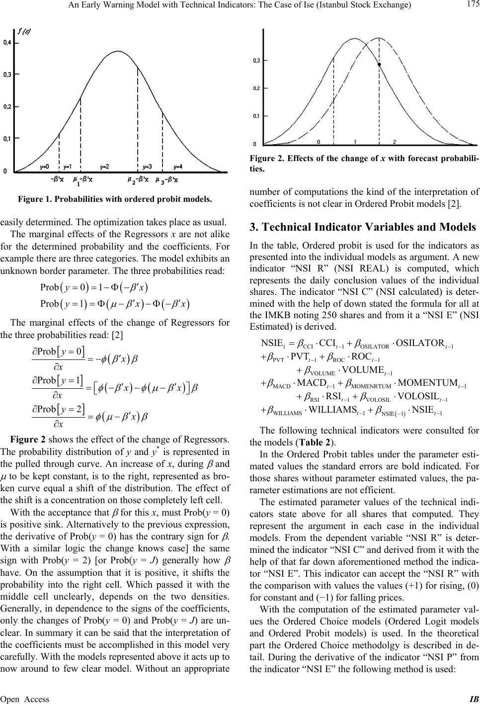

An Early Warning Model with Technical Indicators: The Case of Ise (Istanbul Stock Exchange) 175

Figure 1. Probabilities with ordered probit models.

easily determined. The optimization takes place as usual.

The marginal effects of the Regressors x are not alike

for the determined probability and the coefficients. For

example there are three categories. The model exhibits an

unknown border parameter. The three probabilities read:







 

Prob0 1

Prob 1



 







 



The marginal effects of the change of Regressors for

the three probabilities read: [2]









 





Prob 0

Prob 1

Prob 2

yxx

 





 

 





 

  







 







Figure 2 shows the effect of the change of Regressors.

The probability distribution of y and y* is represented in

the pulled through curve. An increase of x, during



and



to be kept constant, is to the right, represented as bro-

ken curve equal a shift of the distribution. The effect of

the shift is a concentration on those completely left cell.

With the acceptance that



for this x, must Prob(y = 0)

is positive sink. Alternatively to the previous expression,

the derivative of Prob(y = 0) has the contrary sign for



With a similar logic the change knows case] the same

sign with Prob(y = 2) [or Prob(y = J) generally how



have. On the assumption that it is positive, it shifts the

probability into the right cell. Which passed it with the

middle cell unclearly, depends on the two densities.

Generally, in dependence to the signs of the coefficients,

only the changes of Prob(y = 0) and Prob(y = J) are un-

clear. In summary it can be said that the interpretation of

the coefficients must be accomplished in this model very

carefully. With the models represented above it acts up to

now around to few clear model. Without an appropriate

Figure 2. Effects of the change of x with forecast probabili-

ties.

number of computations the kind of the interpretation of

coefficients is not clear in Ordered Probit models [2].

3. Technical Indicator Variables and Models

In the table, Ordered probit is used for the indicators as

presented into the individual models as argument. A new

indicator “NSI R” (NSI REAL) is computed, which

represents the daily conclusion values of the individual

shares. The indicator “NSI C” (NSI calculated) is deter-

mined with the help of down stated the formula for all at

the IMKB noting 250 shares and from it a “NSI E” (NSI

Estimated) is derived.



CCI1 OSILATOR1

PVT1 ROC1

VOLUME 1

MACD1 MOMENRTUM1

RSI1 VOLOSIL1

WILLIAMS 11

NSIE 1

NSIE CCIOSILATOR

PVT ROC

VOLUME

MACD MOMENTUM

RSI VOLOSIL

WILLIAMS NSIE

tt t















 

 



 

The following technical indicators were consulted for

the models (Table 2).

In the Ordered Probit tables under the parameter esti-

mated values the standard errors are bold indicated. For

those shares without parameter estimated values, the pa-

rameter estimations are not efficient.

The estimated parameter values of the technical indi-

cators state above for all shares that computed. They

represent the argument in each case in the individual

models. From the dependent variable “NSI R” is deter-

mined the indicator “NSI C” and derived from it with the

help of that far down aforementioned method the indica-

tor “NSI E”. This indicator can accept the “NSI R” with

the comparison with values the values (+1) for rising, (0)

for constant and (−1) for falling prices.

With the computation of the estimated parameter val-

ues the Ordered Choice models (Ordered Logit models

and Ordered Probit models) is used. In the theoretical

part the Ordered Choice methodolgy is described in de-

tail. During the derivative of the indicator “NSI P” from

the indicator “NSI E” the following method is used:

Open Access IB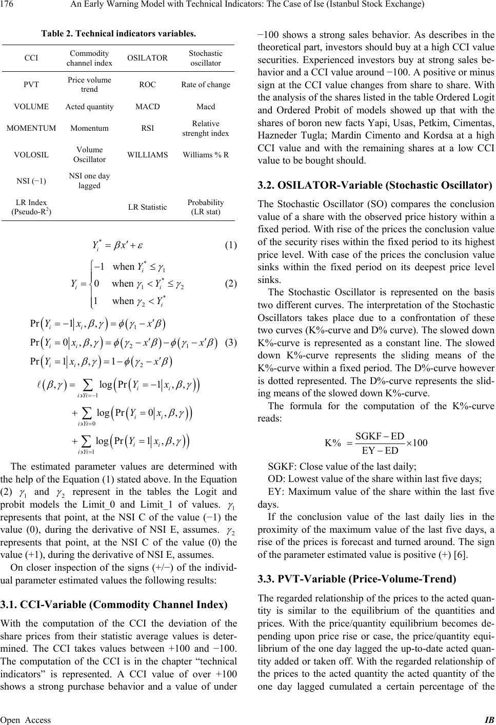

An Early Warning Model with Technical Indicators: The Case of Ise (Istanbul Stock Exchange)

176

Table 2. Technical indicators variables.

CCI Commodity

channel index OSILATOR Stochastic

oscillator

PVT Price volume

trend ROC Rate of change

VOLUME Acted quantity MACD Macd

MOMENTUM Momentum RSI Relative

strenght index

VOLOSIL Volume

Oscillator WILLIAMS Williams % R

NSI (−1) NSI one day

lagged

LR Index

(Pseudo-R2) LR Statistic

Probability

(LR stat)







 (1)

1when

0when

1when



















(2)













Pr1, ,

Pr0, ,

Pr1, ,1

Yx x

Yxx x

Yx x

 



 



 











(3)









,logPr1,

log Pr0,,

log Pr1,,

iYi





















The estimated parameter values are determined with

the help of the Equation (1) stated above. In the Equation

(2) 1



and 2



represent in the tables the Logit and

probit models the Limit_0 and Limit_1 of values. 1



represents that point, at the NSI C of the value (−1) the

value (0), during the derivative of NSI E, assumes. 2



represents that point, at the NSI C of the value (0) the

value (+1), during the derivative of NSI E, assumes.

On closer inspection of the signs (+/−) of the individ-

ual parameter estimated values the following results:

3.1. CCI-Variable (Commodity Channel Index)

With the computation of the CCI the deviation of the

share prices from their statistic average values is deter-

mined. The CCI takes values between +100 and −100.

The computation of the CCI is in the chapter “technical

indicators” is represented. A CCI value of over +100

shows a strong purchase behavior and a value of under

−100 shows a strong sales behavior. As describes in the

theoretical part, investors should buy at a high CCI value

securities. Experienced investors buy at strong sales be-

havior and a CCI value around −100. A positive or minus

sign at the CCI value changes from share to share. With

the analysis of the shares listed in the table Ordered Logit

and Ordered Probit of models showed up that with the

shares of boron new facts Yapi, Usas, Petkim, Cimentas,

Hazneder Tugla; Mardin Cimento and Kordsa at a high

CCI value and with the remaining shares at a low CCI

value to be bought should.

3.2. OSILATOR-Variable (Stochastic Oscillator)

The Stochastic Oscillator (SO) compares the conclusion

value of a share with the observed price history within a

fixed period. With rise of the prices the conclusion value

of the security rises within the fixed period to its highest

price level. With case of the prices the conclusion value

sinks within the fixed period on its deepest price level

sinks.

The Stochastic Oscillator is represented on the basis

two different curves. The interpretation of the Stochastic

Oscillators takes place due to a confrontation of these

two curves (K%-curve and D% curve). The slowed down

K%-curve is represented as a constant line. The slowed

down K%-curve represents the sliding means of the

K%-curve within a fixed period. The D%-curve however

is dotted represented. The D%-curve represents the slid-

ing means of the slowed down K%-curve.

The formula for the computation of the K%-curve

reads:

SGKF ED

K% 100

EY ED







SGKF: Close value of the last daily;

OD: Lowest value of the share within last five days;

EY: Maximum value of the share within the last five

days.

If the conclusion value of the last daily lies in the

proximity of the maximum value of the last five days, a

rise of the prices is forecast and turned around. The sign

of the parameter estimated value is positive (+) [6].

3.3. PVT-Variable (Price-Volume-Trend)

The regarded relationship of the prices to the acted quan-

tity is similar to the equilibrium of the quantities and

prices. With the price/quantity equilibrium becomes de-

pending upon price rise or case, the price/quantity equi-

librium of the one day lagged the up-to-date acted quan-

tity added or taken off. With the regarded relationship of

the prices to the acted quantity the acted quantity of the

one day lagged cumulated a certain percentage of the

Open Access IB

An Early Warning Model with Technical Indicators: The Case of Ise (Istanbul Stock Exchange) 177

up-to-date acted quantity is added or taken off. The per-

centage is calculated as a function of the price rise or

case.

If the acted quantity rises with sinking prices, the PVT

value sinks. In this situation the PVT variable shows a

strong purchase behavior with low prices. Sinking prices

and a sinking quantity are characteristics for one PVT

value any longer not falling. From the negative connec-

tion between acted quantity and rising prices can a minus

sign of the parameter estimated value (−) be derived.

3.4. ROC (Price Rate of Change)

The price adjustment rate (ROC) shows the percent

change of the price of the current daily in the comparison

to the price of the previous daily.

The following formula shows the computation of the

price adjustment rate:



curentcloseclose fordays

Price ROC100

close fordays







If the prices reach a point, also the ROC value reaches

a point. The sign of the parameter estimated value is

negative (−).

3.5. VOLUME (Acted Quantity)

The acted quantity represents the quantity of the bought

and sold shares. The development of the acted quantity

and the prices gives important notes to future events.

With sinking prices are more buyers. By the rise of the

inquired quantity, the prices rise. The sign of the pa-

rameter estimated value is positive (+).

The parameter estimated values of the VOLUME of

indicator for the regarded shares are very small. The rea-

son for it lies to the extent of the acted quantity.

3.6. MACD (Moving Average Convergence

Divergence)

With the help of the MACD trends can be illustrated. The

MACD shows the relationship between two sliding av-

erages, on whose basis purchase and sales decisions can

be met.

With the computation of the MACD first a long-term

and a short term exponentially sliding means are calcu-

lated. Subsequently, from the short term exponentially

sliding means the long-term sliding means is taken off, in

order to determine the MACD. If the short term expo-

nentially sliding means is larger than the long-term ex-

ponentially sliding means, the result is positive and the

MACD lies over the zero-line. This indicates a rise of the

prices. If however the result is negative, the MACD is

under the zero-line.

With the computation among other things the signal

line is determined. This signal line results due to the val-

ues of the exponentially sliding means of the last nine

days. If the MACD cuts the signal line from down up,

then a purchase decision is met. If however the MACD

from above cuts down the signal line, then a sales deci-

sion is met. A rising MACD value is characteristic for a

rising price level. One can interpret a rising MACD value

as sales signal. The sign is negative the parameter esti-

mated value (−).

3.7. Momentum

The Momentum indicates the percent change of the pric-

es within a fixed period. With the help of the Momentum

the profit or loss, which a share obtains within a certain

period, can be represented. The price adjustment rate

(ROC) shows a similar event as the Momentum, the dif-

ference lies in the representational form. The datum line

is with the Momentum with 100 and with the ROC with

0 and on the ordinate the percent change is represented.

The Momentum is computed according to the formula

stated down:

Close value of the last daily

Momentum 100

Close value beforedays





Summarized the Momentum shows the yield of a share

in the comparison to the price before “x” days is obtained.

If the Momentum a maximum value moves reached and

then downward, sales decisions are met. The sign of the

parameter estimated value is negative (−).

3.8. RSI (Relative Strength Index)

With the computation of this characteristic number be-

comes with the help of the “sliding means of the price

movements upward” (MAU Moving AVERAGE UP)

and the “sliding means of the price movements down-

ward” (WAD Moving AVERAGE down) the develop-

ment of the prices determines. The relative Strength in-

dex (RSI) curve takes a value between “0” and “100”.

Following the determination of the MAU and WAD with

the help of a formula of the RSI index is determined. A

rising RSI value means a sinking price history in reverse

and. The sign of the parameter estimated value is nega-

tive (−) [6].

3.9. VOLOSIL (Volume Oscillator)

The volume Oscillator (VOLOSIL) is similar to the Sto-

chastic Oscillator. It becomes instead of for the price, for

which acted quantity computes. The VOLOSIL shows

the difference between the means sliding at short notice

and the means of a security quantity sliding on a long-

Open Access IB

An Early Warning Model with Technical Indicators: The Case of Ise (Istanbul Stock Exchange)

178

term basis. Influence parameters on the VOLOSIL rep-

resent the method of the computation of the sliding

means, the Fristigkeit and the presentation method. The

sign of the parameter estimated value is positive (+).

3.10. WILLIAMS (Williams’ % R)

Williams % R represents a Momentum indicator, by

which levels are represented with multi-purchases and

increased sale. Williams % R is interpreted similarly as

the Stochastic Oscillator. In contrast to the Stochastic

Oscillator has Williams % R a turned sign. If Williams

lies % R between 80% and 100%, then surplus sales find

with the regarded security, at a value between 0% and

20% take place surplus purchases. The purchase and

sales decision should be met only if the security price

moves in the reverse direction. The MACD helps with

the announcement of Share-pries change. A rising Wil-

liams % R marks rising prices. The sign of the parameter

estimated value is positive (+) [7].

3.11. NSI (−1)

“NSI (−1)” represents the material share price adjustment

of the one day lagged. If it takes the value −1, it means

that the value sank and the prices of the current daily can

rise. If the “NSI (−1) is” value of the one day lagged 0 or

+1, then it knows a sinking of the prices meant. The sign

of the parameter estimated value is negative (−).

In the Ordered Logit and Ordered Probit models be-

came instead of the certainty measure of R2 of the LR

index (pseudo R2) and instead of the f-Statistic the LR

Statistic used. Details in addition are in the theoretical

part of this work. The pseudo R2 took very low values.

This is due to the calculation method of the pseudo R2. A

comparison with classical R2-values would not be correct

[8].

In the classical involution model the R2-value between

0 and 1 can move, whereby a value means close 1 a

strong correlation. Dummy Dependent variable model

does not supply value close 1. On the assumption that in

a given interval the correct probabilities of an event are

evenly distributed, it is to be set it possible for R2 an up-

per border of. For this reason a low R2 is not unusual

with the estimation of a linear probability model [9].

4. Emprical Results

Following the four ISE (Istanbul Stock Exchange) indi-

ces are aforementioned the main sector indices (industry,

service, financial and technology sector) and the perti-

nent sub sectors.

The main sector and sub sector indices cover securities,

which are not acted at the stock exchange to note and at

the national market.

CODE INDICES

XU100 ISE NATIONAL-100

XU050 ISE NATIONAL-50

XU030 ISE NATIONAL-30

XKURY ISE CORPORATE GOVERNMENT

XUTUM ISE NATIONAL-ALL SHARES

XUSIN ISE NATIONAL-INDUSTRIALS

XGIDA FOOD, BEVERAGE

XTEKS TEXTILE, LEATHER

XKAGT WOOD, PAPER, PRINTING

XKMYA CHEMICAL, PETROLEUM, PLASTIC

XTAST NON-METAL MINERAL PRODUCTS

XMANA BASIC METAL

XMESY METAL PRODUCTS, MACHINERY

XUHIZ ISE NATIONAL-SERVICES

XELKT ELECTRICITY

XULAS TRANSPORTATION

XTRZM TOURISM

XTCRT WHOLESALE AND RETAIL TRADE

XILTM TELECOMMUNICATIONS

XSPOR SPORTS

XUMAL ISE NATIONAL - FINANCIALS

XBANK BANKS

XSGRT INSURANCE

XFINK LEASING, FACTORING

XHOLD HOLDING AND INVESTMENT

XGMYO REAL ESTATE INVEST.TRUSTS

XUTEK ISE NATIONAL TECHNOLOGY

XBLSM INFORMATION TECHNOLOGY

XSVNM DEFENSE

XYORT ISE INVESTMENT TRUSTS

XIKIU ISE SECOND NATIONAL

XYEKO ISE NEW ECONOMY

Following tables contain some of the significant pa-

rameters of variables in ordered probit models (Tables 3

and 4) [10].

4.1. Stability of the Parameter Estimated Values

The stability of the estimated parameter values, in order

Open Access IB

An Early Warning Model with Technical Indicators: The Case of Ise (Istanbul Stock Exchange)

Open Access IB

179

Table 3. Some of the ordered probit outputs.

ABANA ELEKTRO AK ENERJİ AKTAŞ ELEKTRİK AYEN ENERJİ

SAMPLE

REGRESSION

OUTPUTS

Std.Dev Prob. Std.DevProb. Std. DevProb. Std. DevProb.

N 2116

1585

CCI (−1)

OSILATOR (−1) 0.01 0.00 0.00 0.04 0.02 0.01

PVT (−1)

ROC (−1) −9.34 0.48 0.00

−10.23 2.47 0.00−4.29 0.42 0.00

−21.53 4.50 0.00

VOLUME (−1) 0.00 0.00 0.04

0.00 0.00 0.00

MACD (−1)

0.00 0.00 0.00

MOMENTUM (−1)

−0.27 0.15 0.08

RSI (−1)

0.54 0.25 0.03

VOLOSIL (−1)

WILLIAMS (−1) 0.01 0.00 0.00 0.01 0.00 0.010.01 0.00 0.00 0.01 0.00 0.01

ISARET (−1) −0.07 0.03 0.04 −0.30 0.17 0.08−0.07 0.04 0.06

−0.48 0.20 0.02

LIMIT_0 −0.38 0.04 0.00 −0.29 0.17 0.09−0.73 0.18 0.00

80.38 36.72 0.03

LIMIT_1 0.01 0.04 0.74 0.29 0.17 0.09−0.33 0.18 0.06

81.04 36.74 0.03

LR index

(Pseudo−R2) 0.27

0.24

0.20

0.47

LR statistic 1134.48

42.00

648.45

79.33

Probability (LR stat) 0.00

0.00

HAUPT SEKTOR XUHIZ

XUHIZ

UNTER SEKTOR XELKT

XELKT

Table 4. Summary of models.

Number of

Efficient Estimations % of Total

CCI (−1) 33 13.2

OSILATOR (−1) 108 43.2

PVT (−1) 58 23.2

ROC (−1) 250 100

VOLUME (−1) 214 85.6

MACD (−1) 75 30

MOMENTUM (−1) 27 10.8

RSI (−1) 16 6.4

VOLOSIL (−1) 49 19.6

WILLIAMS (−1) 247 98.8

ISARET (−1) 247 98.8

N (Mean) 1642

LR index (Pseudo-R2)

(Average) 0.24

to be able to make prognoses over the share price change,

tested in the context of this work. For this from 250

shares altogether 32 shares were selected. To the criteria

for choice the number of collections and the affiliation to

at least a sub sector belonged. Shares with the highest

collections from each sub sector each are selected. The

accomplished stability test results are in the following:

With the examination of the stability of the parameter

values of the selected shares at the beginning of a third of

the oldest collections of the parameter computation one

takes out. In a second passage finally only more half of

the collections was located—which recent collections—

for the order, with which a further parameter computa-

tion is accomplished. After Chow a third of the collec-

tions and afterwards half of the collections are taken out

last of the center of the entire elevations. Those only with

the oldest and recent collections the parameter values are

computed. The estimated parameter values with the full

collection number are compared after that far method

with the estimated parameter values, represented down,

with smaller collections and their stability is tested.

An Early Warning Model with Technical Indicators: The Case of Ise (Istanbul Stock Exchange)

180







A t-test was accomplished: 0

stat







By the fulfillment of the condition tstat < ttable the H0

hypothesis is not rejected and the stability of the esti-

mated parameter values of the regarded 32 shares was

confirmed.

The estimated parameter values and stability test de-

termined for the selected 32 shares are in the appendix.

The results displays that the change of the number of

collections do not cause statistic change of the estimated

parameter values.

5. Conclusions

In summary, we can say that during the derivative of NSI

E: NSI C takes the value (−1) assumes that it is smaller

as it is; NSI C takes the value (0) if it lies between; NSI

C takes the value (+1) if it is larger as it is.

For all technical indicators with the computation of the

variables one day lagged, values are used. The conclu-

sion values of 250 shares are raised for the calculations

of the technical indicators. The technical indicators as the

argument were used for the determination of the parame-

ter values, and thereby altogether 250 models are set up.

It participated interesting that the estimated parameter

values of the 250 shares were close. The CCI variable for

33 models, the OSILATOR variable for 108 models, the

PVT variable for 58 models, the ROC variable for all

models, the volume variable for 214 models, the MACD

variable for 75 models, the moment around variable for

27 models, the RSI variable for 16 models, the volume

OS IL variable for 49 models, the WILLIAMS variable

for 247 models and the NSI (−1) variable for 247 models

are efficient.

With those models, in which the technical indicators

represent the arguments, Turkcell, Anadolu Efes and

Ayen Enerji had extreme parameter values. Since the

number of collections is very small with these shares,

one can meet the acceptance that iterated parameter val-

ues are not reached.

5.1. Model Prognoses

With above the 32 shares select for the stability test of

the estimated parameter values, prognoses become for

one period of three months (10 October to 24 January

2007) accomplished. With these prognoses, the “NSI R”

(NSI calculated) of values is determined and derived

from these the “NSI E” (NSI estimated). The derived

“NSI E” of values is compared afterwards with the “NSI

R” (NSI real) values.

Point prognoses and interval prognoses are accom-

plished. In the context of the point prognosis, the values

of “NSI C” were determined with the Limit_0 and

Limit_1 being compared and “NSI E” derives from it.

“NSI C” was under Limit_0 to “NSI P” on (−1) and was

then specified. With the “NSI C” between Limit_0 and

Limit_1, “NSI E” is specified on (0) with a “NSI C” over

Limit_1 on (+1). After derivative of “NSI E”, it is com-

pared with “NSI R” and prognosis accuracy is deter-

mined. In the case of the point, prognoses resulted is

prognosis accuracy between 54 to 72 percent.

For the execution of the interval prognoses, addition-

ally the “NSI still becomes CU” value (NSI calculated

lower one limit) and “the NSI CO” value (NSI calculated

upper one border) is determined. With the help of these

two limit values, during the derivative of the “NSI E”,

the “NSI of EU” values (NSI prognosticated lower ones

limit) and “NSI of EO” values (NSI prognosticated upper

one border) are derived. It was checked whether the “NSI

R”-value is within these two values (between “NSI EU”

and “NSI PO”). With the regarded 32 models (ever a

model per share), “NSI R” is observed within these in-

terval values with a frequency from 70 to 96 percent.

The intervals (“NSI EU” and “NSI EO”) failed some-

times very closely and again very broadly. With very

close intervals (ex.: “NSI EU” = +1 and “NSI EO” = +1).

“NSI E” can speak with the interval borders of safe prog-

noses with the agreement of the point prognosis. On the

other side the interval borders far apart (“NSI EU” = −1

and “NSI EO” = +1) cannot be made safe statements

about the point prognosis “NSI E”. The reason for the far

interval borders lies in the high standard deviation and

the Limit_0 and Limit_1 values, for which again as in-

fluence of external factors is lying far apart, speculation

behavior is responsible.

With the regarded 32 shares, one could observe the in-

terval width of “NSI EU” within the observed period of 3

months = −1 to “NSI EO” = +1 between 9 percent and 83

percent, an average value of 57.4 percent for 32 shares

results. “NSI EU” = +1 to “NSI EO” = +1 was observed

with the 32 shares within the period by 3 months with a

frequency from 5.5 to 62.5 percent, and resulted in an

average value of 20.1 percent. When agreeing the “NSI

E”, “NSI EU” and “NSI EO” value an agreement with

“NSI R” which is determined between 61 and 100 per-

cent, i.e. with an average value of 89 percent.

In principle, one can say that with all securities with

18 (= 0.201 * 0.89) percent of probability safe prognoses

can be accomplished. In summary, we can say that one

with 63 percent of correct point prognoses altogether

with approx. 57 percent of all prognoses about no safe pro-

gnoses to talk can lie apart, and there the interval borders

far and with approx. 18 percent about safe prognoses to

tal can lie apart. 25 percent of the remaining can be k

Open Access IB

An Early Warning Model with Technical Indicators: The Case of Ise (Istanbul Stock Exchange)

Open Access IB

181

Table 5. Point and interval prognoses.

Stock

NSI E

Correct

Interval

Estimation Correct

NSI E = NSI

EU = NSI EO

NSI E = NSI EU =

NSI EO Correct

NSI PU = −1 NSI PO = +1

NSI P Betwixt

İŞ BANKASI (C) Amount43 67 13 11 43

in % 60.56 94.37 18.31 84.62 60.56

YAPI VE KREDİ BANK. Amount46 67 17 15 35

in % 64.79 94.37 23.94 88.24 49.30

İKTİSAT FİN. KİR. Amount42 66 16 14 37

in % 59.15 92.96 22.54 87.50 52.11

VAKIF GMYO Amount39 64 8 6 48

in % 57.35 94.12 11.76 75.00 70.59

ALARKO HOLDİNG Amount43 66 18 16 37

in % 60.56 92.96 25.35 88.89 52.11

ENKA HOLDİNG Amount56 76 12 11 53

in % 72.73 98.70 15.58 91.67 68.83

KOÇ HOLDİNG Amount41 69 17 14 38

in % 56.94 95.83 23.61 82.35 52.78

ANADOLU SİGORTA Amount39 51 45 37 7

in % 54.17 70.83 62.50 82.22 9.72

ANADOLU GIDA Amount45 67 13 8 39

in % 65.22 97.10 18.84 61.54 56.52

MARET Amount47 71 17 16 34

in % 65.28 98.61 23.61 94.12 47.22

PINAR SU Amount50 71 5 4 60

in % 69.44 98.61 6.94 80.00 83.33

AYGAZ Amount45 70 11 10 38

in % 62.50 97.22 15.28 90.91 52.78

BRİSA Amount44 66 22 18 36

in % 62.86 94.29 31.43 81.82 51.43

ECZACIBAŞI İLAÇ Amount49 71 15 15 56

in % 69.01 100.00 21.13 100.00 78.87

PETKİM Amount44 70 14 14 43

in % 61.11 97.22 19.44 100.00 59.72

ÇELİK HALAT Amount46 72 8 8 49

in % 63.89 100.00 11.11 100.00 68.06

EREĞLİ DEMİR CELİK Amount52 70 13 12 42

in % 72.22 97.22 18.06 92.31 58.33

SARKUYSAN Amount51 68 12 12 37

in % 70.83 94.44 16.67 100.00 51.39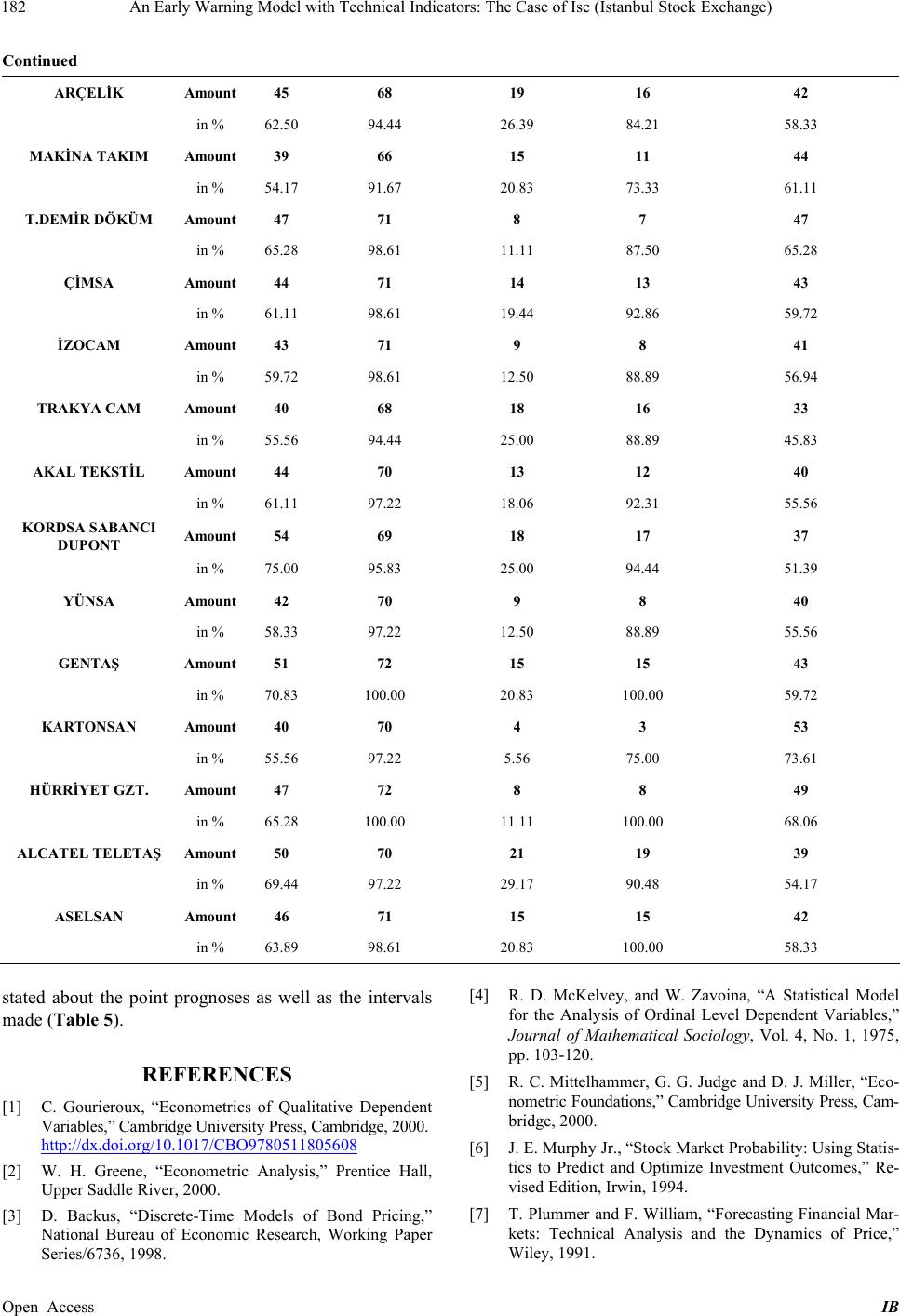

An Early Warning Model with Technical Indicators: The Case of Ise (Istanbul Stock Exchange)

182

Continued

ARÇELİK Amount45 68 19 16 42

in % 62.50 94.44 26.39 84.21 58.33

MAKİNA TAKIM Amount39 66 15 11 44

in % 54.17 91.67 20.83 73.33 61.11

T.DEMİR DÖKÜM Amount47 71 8 7 47

in % 65.28 98.61 11.11 87.50 65.28

ÇİMSA Amount44 71 14 13 43

in % 61.11 98.61 19.44 92.86 59.72

İZOCAM Amount43 71 9 8 41

in % 59.72 98.61 12.50 88.89 56.94

TRAKYA CAM Amount40 68 18 16 33

in % 55.56 94.44 25.00 88.89 45.83

AKAL TEKSTİL Amount44 70 13 12 40

in % 61.11 97.22 18.06 92.31 55.56

KORDSA SABANCI

DUPONT Amount54 69 18 17 37

in % 75.00 95.83 25.00 94.44 51.39

YÜNSA Amount42 70 9 8 40

in % 58.33 97.22 12.50 88.89 55.56

GENTAŞ Amount51 72 15 15 43

in % 70.83 100.00 20.83 100.00 59.72

KARTONSAN Amount40 70 4 3 53

in % 55.56 97.22 5.56 75.00 73.61

HÜRRİYET GZT. Amount47 72 8 8 49

in % 65.28 100.00 11.11 100.00 68.06

ALCATEL TELETAŞ Amount50 70 21 19 39

in % 69.44 97.22 29.17 90.48 54.17

ASELSAN Amount46 71 15 15 42

in % 63.89 98.61 20.83 100.00 58.33

stated about the point prognoses as well as the intervals

made (Table 5).

REFERENCES

[1] C. Gourieroux, “Econometrics of Qualitative Dependent

Variables,” Cambridge University Press, Cambridge, 2000.

http://dx.doi.org/10.1017/CBO9780511805608

[2] W. H. Greene, “Econometric Analysis,” Prentice Hall,

Upper Saddle River, 2000.

[3] D. Backus, “Discrete-Time Models of Bond Pricing,”

National Bureau of Economic Research, Working Paper

Series/6736, 1998.

[4] R. D. McKelvey, and W. Zavoina, “A Statistical Model

for the Analysis of Ordinal Level Dependent Variables,”

Journal of Mathematical Sociology, Vol. 4, No. 1, 1975,

pp. 103-120.

[5] R. C. Mittelhammer, G. G. Judge and D. J. Miller, “Eco-

nometric Foundations,” Cambridge University Press, Cam-

bridge, 2000.

[6] J. E. Murphy Jr., “Stock Market Probability: Using Statis-

tics to Predict and Optimize Investment Outcomes,” Re-

vised Edition, Irwin, 1994.

[7] T. Plummer and F. William, “Forecasting Financial Mar-

kets: Technical Analysis and the Dynamics of Price,”

Wiley, 1991.

Open Access IB

An Early Warning Model with Technical Indicators: The Case of Ise (Istanbul Stock Exchange) 183

[8] T. Laitila, “A Pseudo-R2 Measure for Limited and Quali-

tative Dependent Variable Models,” Journal of Econo-

metrics, Vol. 56, No. 3, 1993, pp. 341-345.

[9] R. S. Pindyck and D. L. Rubinfeld, “Econometric Models

and Economic Forecasts,” McGraw-Hill, 1998.

[10] IMKB, 2001. http://www.imkb.gov.tr/endeksler.htm

Open Access IB