The 3D Computer Image of the Anterior Corneal Surface

doi:10.4236/eng.2013.510B098

Paper Menu >>

Journal Menu >>

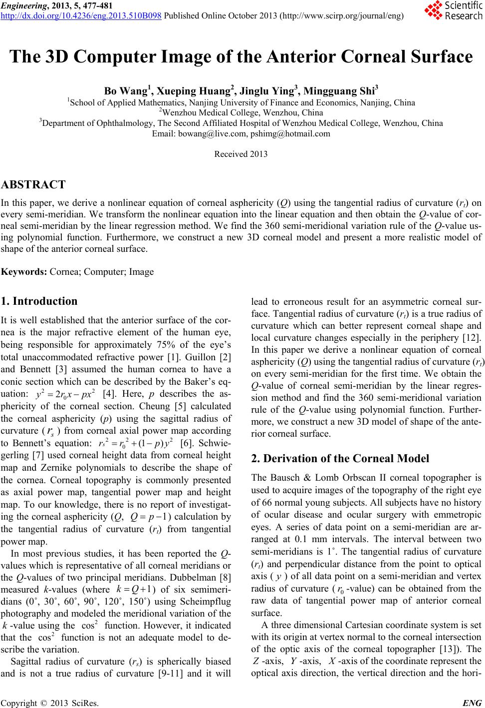Engineering, 2013, 5, 477-481

http://dx.doi.org/10.4236/eng.2013.510B098 Published Online October 2013 (http://www.scirp.org/journal/eng)

The 3D Computer Image of the Anterior Corneal Surface

Bo Wang1, Xueping Huang2, Jinglu Ying3, Mingguang Shi3

1School of Applied Mathematics, Nanjing University of Finance and Economics, Nanjing, China

2Wenzhou Medical College, Wenzhou, China

3Department of Ophthalmology, The Second Affiliated Hospital of Wenzhou Medical College, Wenzhou, China

Email: bowa ng@live.com, [email protected]

Received 2013

ABSTRACT

In this paper, we derive a nonlinear equation of corneal asphericity (Q) using the tangential radius of curvature (rt) on

every semi-meridian. We transform the nonlinear equation into the linear equation and then obtain the Q-value of cor-

neal semi-meridian by the linear regression method. We find the 360 semi-meridional v ariation rule of the Q-value us-

ing polynomial function. Furthermore, we construct a new 3D corneal model and present a more realistic model of

shape of the anterior corneal surface.

Keywords: Cornea; Computer; Image

1. Introduction

It is well established that the anterior surface of the cor-

nea is the major refractive element of the human eye,

being responsible for approximately 75% of the eye’s

total unaccommodated refractive power [1]. Guillon [2]

and Bennett [3] assumed the human cornea to have a

conic section which can be described by the Baker’s eq-

uation:

2yr xpx= −

[4]. Here, p describes the as-

phericity of the corneal section. Cheung [5] calculated

the corneal asphericity (p) using the sagittal radius of

curvature (

) from corneal axial power map according

to Bennett’s equation:

22 2

(1 )

r rpy= +−

[6]. Schwie-

gerling [7] used corneal height data from corneal height

map and Zernike polynomials to describe the shape of

the cornea. Corneal topography is commonly presented

as axial power map, tangential power map and height

map. To our knowledge, there is no report of investigat-

ing the corneal asphericity (Q,

1Qp= −

) calculation by

the tangential radius of curvature (rt) from tangential

power map.

In most previous studies, it has been reported the Q-

values which is representative of all corneal meridians or

the Q-values of two principal meridians. Dubbelman [8]

measured k-values (where

1kQ= +

) of six semimeri-

dians (0˚, 30˚, 60˚, 90˚, 120˚, 150˚) using Scheimpflug

photograph y and modeled the meridional variatio n of the

-value using the

cos

function. However, it indicated

that the

cos

function is not an adequate model to de-

scribe t he va riati on.

Sagittal radius of curvature (rs) is spherically biased

and is not a true radius of curvature [9-11] and it will

lead to erroneous result for an asymmetric corneal sur-

face. Tangential radius of curvature (rt) is a true radius of

curvature which can better represent corneal shape and

local curvature changes especially in the periphery [12].

In this paper we derive a nonlinear equation of corneal

asphericity (Q) using the tangential radius of curvature (rt)

on every semi-meridian for the first time. We obtain the

Q-value of corneal semi-meridian by the linear regres-

sion method and find the 360 semi-meridional variation

rule of the Q-value using polynomial function. Further-

more, we construct a new 3D model of shape of the ante-

rior corneal surface.

2. Derivation of the Corneal Model

The Bausch & Lomb Orbscan II corneal topographer is

used to acquire images of the topography of the right eye

of 66 normal young subj ects. All subj ec ts have no history

of ocular disease and ocular surgery with emmetropic

eyes. A series of data point on a semi-meridian are ar-

ranged at 0.1 mm intervals. The interval between two

semi-meridians is 1˚. The tangential radius of curvature

(rt) and perpendicular distance from the point to optical

axis (

) of all data point on a se mi-meridian and vertex

radius of curvature (

-value) can be obtained from the

raw data of tangential power map of anterior corneal

surface.

A three dimensional Car tesian coordinate system is set

with its origin at vertex nor mal to the corn eal interse ction

of the optic axis of the corneal topographer [13]). The

-axis,

-axis of the coordinate represent the

optical axis direction, the vertical direction and the hori-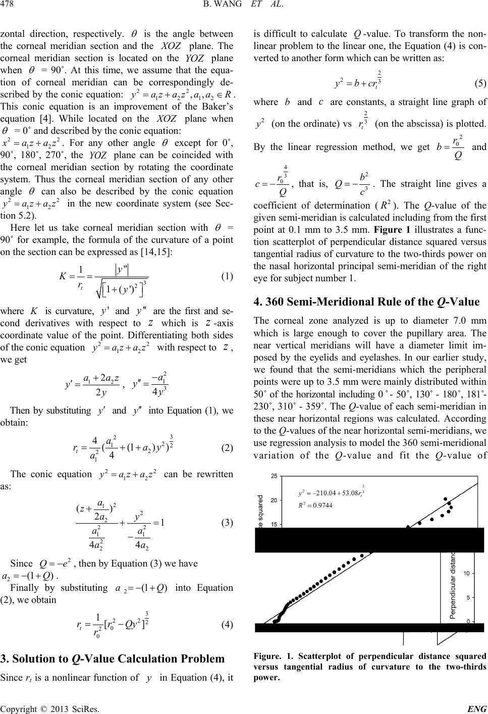

B. WANG ET AL.

478

zontal direction, respectively.

is the angle between

the corneal meridian section and the

XOZ

plane. The

corneal meridian section is located on the

YOZ

plane

when

= 90˚. At this time, we assume that the equa-

tion of corneal meridian can be correspondingly de-

scribed by the conic equation:

12 12

,,yazaza aR=+∈

This conic equation is an improvement of the Baker’s

equation [4]. While located on the

XOZ

plane when

= 0˚ and described by the conic equation:

xaz az= +

. For any other angle

except for 0˚,

90˚, 180˚, 270˚, the

YOZ

plane can be coincided with

the corneal meridian section by rotating the coordinate

system. Thus the corneal meridian section of any other

angle

can also be described by the conic equation

yaz az= +

in the new coordinate system (see Sec-

tion 5.2) .

Here let us take corneal meridian section with

90˚ for example, the formula of the curvature of a point

on the section can be expressed as [14,15]:

1( ')

Kry

= =





(1)

where

is curvature,

and

''y

are the first and se-

cond derivatives with respect to

which is

-axis

coordinate value of the point. Differentiating both sides

of the conic equation

yaz az= +

with respect to

we get

a az

′=

−

′′ =

Then by substituting

y′

and

y′′

into Equation (1), we

obtain:

4((1) )

r ay

= ++

(2)

The conic equation

yaz az= +

can be rewritten

as:

()

zay

−

(3)

Since

Qe= −

, then by Equation (3) we have

(1 )aQ=−+

Finally by substituting

(1 )aQ=−+

into Equation

(2), we obtain

1[]

rr Qy

= −

(4)

3. Solution to Q-Value Calculation Problem

Since rt is a nonlinear function of

in Equation (4), it

is difficult to calculate

-value. To transform the non-

linear problem to the linear one, the Equation (4) is con-

verted to another form which can be written as:

yb cr= +

(5)

where

and

are constants, a straight line graph of

(on the ordinate) vs

(on the abscissa) is plotted.

By the linear regression method, we get

and

= −

, that is,

= −

. The straight line gives a

coefficient of determination (2

). The Q-value of the

given semi-meridian is calculated includ ing from the first

point at 0.1 mm to 3.5 mm. Figure 1 illustrates a func-

tion scatterplot of perpendicular distance squared versus

tangential radius of curvature to the two-thirds power on

the nasal horizontal principal semi-meridian of the right

eye for subject number 1.

4. 360 Semi-Meridional Rule of the Q-Value

The corneal zone analyzed is up to diameter 7.0 mm

which is large enough to cover the pupillary area. The

near vertical meridians will have a diameter limit im-

posed by the eyelids and eyelashes. In our earlier study,

we found that the semi-meridians which the peripheral

points wer e up to 3.5 mm were mainly distributed within

50˚ of the horizontal including 0˚ - 50˚, 130˚ - 180˚, 181˚-

230˚, 310˚ - 359˚. The Q-value of each semi-meridian in

these near horizontal regions was calculated. According

to the Q-values of the near horizontal semi-meridians, we

use regression analysis to model the 360 semi-meridional

variation of the Q-value and fit the Q-value of

Figure. 1. Scatterplot of perpendicular distance squared

versus tangential radius of curvature to the two-thirds

power.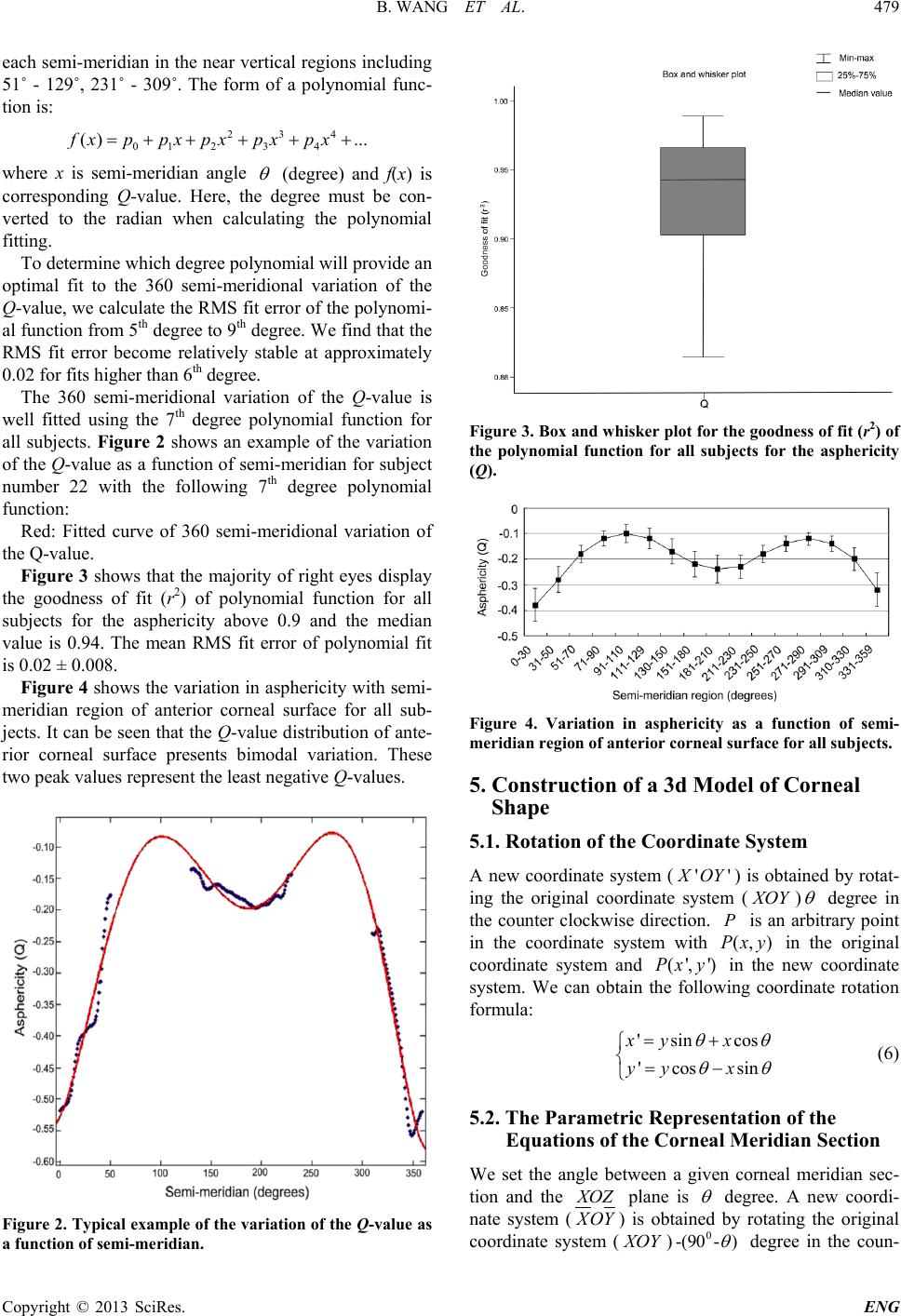

B. WANG ET AL.

479

each semi-meridian in the near vertical regions including

51˚ - 129˚, 231˚ - 309˚. The form of a polynomial func-

tion is:

234

01 234

( )...f xppxpxpxpx=+++++

where x is semi-meridian angle

(degree) and f(x) is

corresponding Q-value. Here, the degree must be con-

verted to the radian when calculating the polynomial

fitting.

To determine which degree polynomial will provide an

optimal fit to the 360 semi-meridional variation of the

Q-value, we calculate the RMS fit error of the polynomi-

al function from 5th degree to 9th degree. We find that the

RMS fit error become relatively stable at approximately

0.02 for fits higher than 6th degree.

The 360 semi-meridional variation of the Q-value is

well fitted using the 7th degree polynomial function for

all subjects. Figure 2 shows an example of the variation

of the Q-value as a function of semi-meridian for subject

number 22 with the following 7th degree polynomial

function:

Red: Fitted curve of 360 semi-meridional variation of

the Q-value.

Figure 3 shows that the majority of right eyes display

the goodness of fit (r2) of polynomial function for all

subjects for the asphericity above 0.9 and the median

value is 0.94. The mean RMS fit error of polynomial fit

is 0.02 ± 0.008.

Figure 4 shows the variation in asphericity with semi-

meridian region of anterior corneal surface for all sub-

jects. It can be seen that the Q-value distribution of ante-

rior corneal surface presents bimodal variation. These

two peak va l ues repres ent the l e a s t negative Q-values.

Figure 2. Typical example of the variation of the Q-value as

a function of semi-meridian.

Figure 3. Box and whisker plot for the goodness of fit (r2) of

the polynomial function for all subjects for the asphericity

(Q).

Figure 4. Variation in asphericity as a function of semi-

meridian region of anterio r corneal surface for all subjects.

5. Construction of a 3d Model of Corneal

Shape

5.1. Rotation of the Coordinate System

A new coordinate system (

''X OY

) is obtained by rotat-

ing the original coordinate system (

XOY

)

degree in

the counter clockwise direction.

is an arbitrary point

in the coordinate system with

(, )Pxy

in the original

coordinate system and

( ',')Px y

in the new coordinate

system. We can obtain the following coordinate rotation

formula:

' sincos

' cossin

xy x

yy x

θθ

= +



= −



(6)

5.2. The Parametric Representation of the

Equations of the Corneal Meridian Section

We set the angle between a given corneal meridian sec-

tion and the

XOZ

plane is

degree. A new coordi-

nate system (

XOY

) is obtained by rotating the original

coordinate system (

XOY

)

-(90 -)

degree in the coun-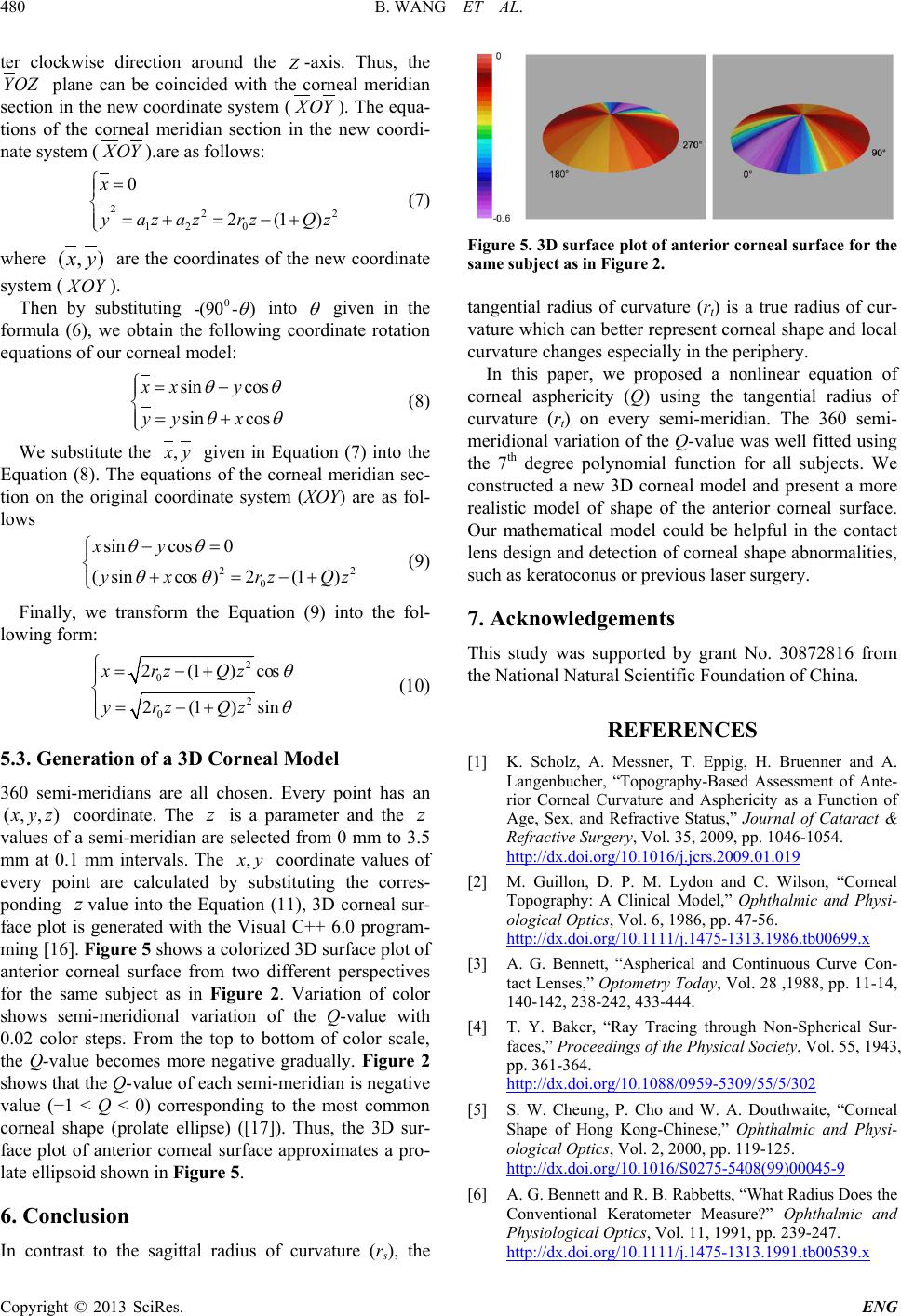

B. WANG ET AL.

480

ter clockwise direction around the

-axis. Thus, the

YOZ

plane can be coincided with the corneal meridian

section in the new coordinate system (

XOY

). The equa-

tions of the corneal meridian section in the new coordi-

nate system (

XOY

).are as follows:

222

12 0

2(1 )

yaz azrzQz

=



= +=−+





(7)

where

(, )xy

are the coordinates of the new coordinate

system (

XOY

Then by substituting

-(90 -)

into

given in the

formula (6), we obtain the following coordinate rotation

equations of our corneal model:

sin cos

xx y

yy x

θθ

= −



= +





(8)

We substitute the

,xy

given in Equation (7) into the

Equation (8). The equations of the corneal meridian sec-

tion on the original coordinate system (XOY) are as fol-

lows

sincos 0

( sincos)2(1)

yxrz Qz

θθ

−=





+= −+





(9)

Finally, we transform the Equation (9) into the fol-

lowing f orm:

2(1)cos

2(1)sin

x rzQz

y rzQz

= −+





= −+



(10)

5.3. Generation of a 3D Corneal Model

360 semi-meridians are all chosen. Every point has an

(,,)xyz

coordinate. The

is a parameter and the

values of a semi-meridian are selected from 0 mm to 3.5

mm at 0.1 mm intervals. The

,xy

coordinate values of

every point are calculated by substituting the corres-

ponding

value into the Equation (11), 3D corneal sur-

face plot is generated with the Visual C++ 6.0 program-

ming [16]. Figure 5 shows a colorized 3D surface plo t of

anterior corneal surface from two different perspectives

for the same subject as in Figure 2. Variation of color

shows semi-meridional variation of the Q-value with

0.02 color steps. From the top to bottom of color scale,

the Q-value becomes more negative gradually. Figure 2

shows that the Q-value of each semi-meridian is negative

value (−1 < Q < 0) corresponding to the most common

corneal shape (prolate ellipse) ([17]). Thus, the 3D sur-

face plot of anterior corneal surface approximates a pro-

late ellipsoid shown in Figu re 5.

6. Conclusion

In contrast to the sagittal radius of curvature (rs), the

Figure 5. 3D surface plot of anterior corneal surface for the

same subject as in Figure 2.

tangential radius of curvature (rt) is a true radius of cur-

vature which can better represent corneal shape and local

curvature changes especially in the periphery.

In this paper, we proposed a nonlinear equation of

corneal asphericity (Q) using the tangential radius of

curvature (rt) on every semi-meridian. The 360 semi-

meridional variation of the Q-value was well fitted using

the 7th degree polynomial function for all subjects. We

constructed a new 3D corneal model and present a more

realistic model of shape of the anterior corneal surface.

Our mathematical model could be helpful in the contact

lens design and detection of corneal shape abnormalities,

such as kerat oconus or previous la s er surger y.

7. Acknowledgements

This study was supported by grant No. 30872816 from

the National Natural Scientific Found a tion of China.

REFERENCES

[1] K. Scholz, A. Messner, T. Eppig, H. Bruenner and A.

Langenbucher, “Topography-Based Assessment of Ante-

rior Corneal Curvature and Asphericity as a Function of

Age, Sex, and Refractive Status,” Journal of Cataract &

Refractive Surgery, Vol. 35, 2009, pp. 1046-1054.

http://dx.doi.org/10.1016/j.jcrs.2009.01.019

[2] M. Guillon, D. P. M. Lydon and C. Wilson, “Corneal

Topography: A Clinical Model,” Ophthalmic and Physi-

ological Optics, Vol. 6, 1986, pp. 47-56.

http://dx.doi.org/10.1111/j.1475-1313.1986.tb00699.x

[3] A. G. Bennett, “Aspherical and Continuous Curve Con-

tact Lenses,” Optometry Today, Vol. 28 ,1988, pp. 11-14,

140-142, 238-242, 433-444.

[4] T. Y. Baker, “Ray Tracing through Non-Spherical Sur-

faces,” Proceedings of the Physical Society, Vol. 55, 1943,

pp. 361-364.

http://dx.doi.org/10.1088/0959-5309/55/5/302

[5] S. W. Cheung, P. Cho and W. A. Douthwaite, “Corneal

Shape of Hong Kong-Chinese,” Ophthalmic and Physi-

ological Optics, Vol. 2, 2000, pp. 119-125.

http://dx.doi.org/10.1016/S0275-5408(99)00045-9

[6] A. G. Bennett and R. B. Rabbetts, “What Radi us Does the

Conventional Keratometer Measure?” Ophthalmic and

Physiological Optics, Vol. 11, 1991, pp. 239-247.

http://dx.doi.org/10.1111/j.1475-1313.1991.tb00539.x

B. WANG ET AL.

481

[7] J. Schwiegerling and J. E. Greivenkamp, “Using Corneal

Height Maps and Polynomial Decomposition to Deter-

mine Corneal Aberrations,” Optometry and Vision Science

Journal, Vol. 74, 1997, pp. 906-916.

http://dx.doi.org/10.1097/00006324-199711000-00024

[8] M. Dubbelman, V. A. D. P. Sicam and G. L. Van der

Heijde, “The Shape of the Anterior and Posterior Surface

of the Aging Human Cornea,” Vision Research, Vol. 46,

2006, pp. 993-1001.

http://dx.doi.org/10.1016/j.visres.2005.09.021

[9] C. Roberts, “Characterization of the Inherent Error in a

Spherically-Biased Corneal Topography System in Map-

ping a Radially Aspheric Surface,” Journal of Cataract &

Refractive Surgery, Vol. 10, 1994, pp. 103-111.

[10] C. Roberts, “Analysis of t he Inherent Error of the TMS-1

Topographic Modeling System in Mapping a Radially

Aspheric Surface,” Cornea, Vol. 14, 1995, pp. 258-265.

http://dx.doi.org/10.1097/00003226-199505000-00006

[11] J. S. Chan, R. B. Mandell, D. S. Burger and R. E. Fusaro,

“Accuracy of Videokeratography for Instantaneous Ra-

dius in Keratoconus,” Optometry and Vision Science

Journal, Vol. 72 , No. 11, 1995, pp. 793-799.

http://dx.doi.org/10.1097/00006324-199511000-00004

[12] L. B. Szczotka and J. Thomas, “Comparison of Axial and

Instantaneous Videokeratographic Data in Keratoconus

and Utility in Contact Lens Curvature Prediction,” The

CLAO Journal, Vol. 24, 1998, pp. 22-28.

[13] R. B. Mandell, C. S. Chiang and S. A. Klein, “Location of

the Major Corneal Reference Points,” Optometry and Vi-

sion Science Journal, Vol. 72, 1995, pp. 776-784.

http://dx.doi.org/10.1097/00006324-199511000-00002

[14] A. Gray, “Modern Differential Geometry of Curves and

Surfaces with Mathematica,” 2nd Edition, CRC Press,

Boca Raton, 1997.

[15] E. Kreyszig, “Differential Geometry,” Dover, New York,

1991.

[16] J. D. Foley, A. V. Dam, S. K. Feiner and J. F. Hughes,

“Computer Graphics: Principles and Practice in C,” 2nd

Edition, Addison-Wesley, Boston, 1995.

[17] P. M. Kiely, G. Smith and L. G. Carney, “The Mean

Shape of the Human Cornea,” Optica Acta, Vol. 29, 1982,

pp. 1027-1040. http://dx.doi.org/10.1080/713820960