The Solutions for the Eco-Epidemic Model with Homotopy Analysis Method

doi:10.4236/eng.2013.510B091

Paper Menu >>

Journal Menu >>

Engineering, 2013, 5, 446-449

http://dx.doi.org/10.4236/eng.2013.510B091 Published Online October 2013 (http://www.scirp.org/journal/eng)

The Solutions for the Eco-Epidemic Model with Homotopy

Analysis Method

Xiurong Chen

Department of Science and Information, Qingdao Agricultural University, Qingdao, China

Email: [email protected]

Received 2013

ABSTRACT

In this paper, the Homotopy Analysis Method (HAM) has been used to solve an eco-epidemic model equation. The al-

gorithm of approximate analytical solution is obtained. HAM contains the auxiliary parameter h which provides us with

a convenient way to adjust and control convergence region and rate of solution series. The results obtained show that

these algorithms are accurate and efficient for the model.

Keywords: Nonlinear Partial Differential Equations; Homotopy Analy s i s Method; Eco-Epidemic Equations

1. Introduction

There has recently been much attention devoted to the

search for better and more efficient solution methods for

determining a solution, approximate or exact, analytical

or numerical, to nonlinear models. Finding approximate

solutions of these nonlinear equations is interesting and

important. Many methods have been developed to solve

nonlinear partial differential equations (NPDEs) such as

biologically-based technologies [1], Adomian decompo-

sition method [2], homotopy perturbation method [3], and

so on.

The HAM first envisioned by Liao [4], is another po-

werful analytical method for nonlinear problem. Many

authors have applied the HAM for solving nonlinear eq-

uations in [5], for solving solitary waves with discontinu-

ity in [6], for s eri e s s olutions of nano boundary layer flows

in [7], for nonlinear equations in [8] and many other

subjects. The technique employed here is very powerful

and has been already successfully applied to various com-

plicated problems [9-13]. Thus, through HAM, explicit

analytic solutions of nonlinear problems are possible.

The application of the HAM in engineering problems

in highly considered by scientists, because HAM pro-

vides us with a convenient way to control the conver-

gence of approximation series, which is a fundamental

qualitative difference in analysis between HAM and oth-

er methods. The purpose of this paper is to implement

HAM to eco-epidemic model equations [1]:

1 12

()

xr xaxbxybxz

yry cxy dyyzyz

zyzd zyz

′=−− −

′= +−+−



′=−+



(1)

where

(),(), ()xtyt zt

are the density of a wild p lant spe-

cies, a susceptible pest and infected pest which live on

the crop. All parameters are positive cons tants.

2. The Solution by Ham

Note

12 13 2121

, ,,,,aaab abbcbd=====

= +

= −

, this leads to the dimensionless equations

11 23

21 23

xr xaxaxyaxz

yryb xybybyz

zd yzdz

′=−−−



′=+− −





′= −



(2)

with the initial conditions

123

(0),(0), (0)x Ay Az A= = =

Due to the governing Equation (2), w e choose the aux-

iliary linear operators as follows:

(; )

[(;)]Xtp

LXtp t

∂

=∂

(3.1)

(; )

[( ;)]Ytp

LYtp t

∂

=∂

(3.2)

(; )

[( ;)]Ztp

L Ztpt

∂

=∂

(3.3)

which satisfy

[]0LC =

(4)

where

and

are integral constants, and the

(; ),(; ),(; )XtpYtp Ztp

are real functions. Furthermore,

due to (2), we define the non-linear operators

X. R. CHEN

447

111 23

[,,]NXYZXrXaXaXYaXZ

′

=−+ ++

(5.1)

22123

[,,]NXYZYrYbXYbYb YZ

′

=−−+ +

(5.2)

3 12

[,,]NXYZZd YZdZ

′

=−+

(5.3)

Then, introducing a non-zero auxiliary h, we construct

the zero-order deformation equations

10111

(1)[(; )()]()[,, ]pLXtpxthHtpNXYY− −=

(6.1)

2022 2

(1)[(;)()]()[,,]pLYtpy thHtpNXYY− −=

(6.2)

3033 3

(1)[ (;)()]()[, ,]pLZtpz thHtpNXYY− −=

(6.3)

Obviously, when

0p=

and

1p=

, we have the so-

lutions

000

( ;0)( ),(;0)(),(;0)( )XtxtYtytZtzt= ==

, (7)

( ;1)( ),( ;1)( ),( ;1)( )XtxtYtytZtzt= ==

(8)

Therefore, as the embedding parameter p increases

from 0 to 1,

(; ),(; )XtpYtp

and

(; )Ztp

vary from the

initials

(), ()xtyt

and

()zt

to the exa c t s o lu ti on

()xt

()yt

and

()zt

governed by (2). This is the basic idea

of the homotopy and this kind of variation is called de-

formations in topology.

Thus, by Taylor’s theorem and (7), we can express

( ,,)()()

Xxtpx tx tp

∞

= +

∑

(9.1 )

( ,,)()()

Yxtpy ty tp

∞

=+∑

(9.2 )

( ,,)()()

Zxtpz tz tp

∞

= +

∑

(9.3 )

where

1(;)

() !

Xtp

xt kp

∂

=∂

(10.1)

1(; )

(,)!

Ytp

y xtkp=

∂

=∂ (10.2)

1(; )

(,)!

Ztp

z xtkp=

∂

=∂ (10.3)

If the auxiliary linear parameter, the initial conditions,

and the auxiliary parameters

123

,,hhh

( ),(),HtHt

()Ht

are chosen, the above series converge at

1p=

and one has

() ()()

xtx txt

∞

=+ ∑

(11 .1 )

() ()()

yty ty t

∞

= +

∑

(11 .2 )

() ()()

ztz tzt

∞

= +

∑

(11 .3 )

Let

123

hhhh== =

and

123

()()()1HtHtHt== =

Differentiating the zero-order deformation Equations (6)

m times with resp ect to p and then dividing them by

and finally setting

0p=

, the mth-order deformation

equations read

111 111

[ ()()][,,]

mmmm mmm

L xtxthRxyz

−− −−

−=

(12.1)

212 111

[ ()()][,,]

mmmm mmm

L ytythRxyz

−− −−

−=

(12.2)

313 111

[ ()()][,,]

mmmm mmm

L ztzthRxyz

−− −−

−=

(12.3)

with the initial conditions (

1m≥

)

(0) 0,(0) 0,(0) 0

mmm

xyy===

(13)

where

1111 1121

()

m m mjmjjmj

jmj

Rtxrxax xaxy

a xz

−−

− −−−−−

= =

−

−−

′

=−+ +

∑∑

∑

(14.1)

2111121

()

mmrmjm jjm j

jmj

R tyrybxybyy

b xz

−−

− −−−−−

= =

−

−−

′

=−− +

∑∑

∑

(14.2)

3111 21

()

mmjm jjmj

R tzdyzdzz

−−

− −−−−

= =

′

=−+

∑∑

(14.3)

and



=≤



(15)

Now, the solutions of the mth-order deformation Equ-

ations (12) for

1m≥

become

()

m mmm

xxhR d

χ ττ

−

= +

∫

(16.1)

()

m mmm

yy hR d

χ ττ

−

=+ ∫

(16.2)

0()

m mmm

zz hRd

χ ττ

−

=+ ∫

(16.3 )

Mathematica software is used to solve the linear Equa-

tions (16) under the initial conditions up to first few or-

der of approxim a t ions. We ha ve :

()xt A=

;

()yt A=

;

()zt A=

(17)

1 11

()xthAhtE= +

(1 8.1)

1 21

()y thAhtF=+

(18 .2 )

1 31

()z thAhtH= +

(18 .3 )

2 22

211 2122

()(1 )(1 )xthhAhhtEh tEh tE=+++++

(19.1)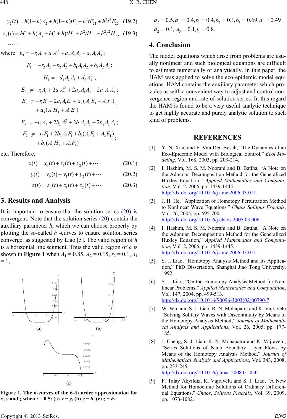

X. R. CHEN

448

2 22

2212122

()(1 )(1 )ythhAhhtFh tFh tF=+++++

(19.2)

2 22

231 2122

()(1 )(1 )zthhAhhtHh tHh tH=+++++

(19.3)



where

111 11212313

ErAaAa AAaAA=−+ ++

;

122 22112323

F rAbAbAAbAA=−+ ++

;

112323

HdAA dA=−+

;

21 1111212313

22 2ErAaAa AAaAA=−+ ++

;

22111112 2111

31 131

2( )

()

ErEaAEa AEAF

a AHAE

=−+ +−

;

21 2222112323

22 2FrAbAbAAbAA=−+ ++

;

22212 2111121

32131

2( )

()

FrFbAFbAFAE

b AHAF

=−++ +

++ ;

etc. Therefore,

012

()() ()()xtxtxtxt=+++

(20.1)

012

()() ()()ytytytyt= +++

(20.2 )

012

()()()()ztztztzt= +++

(20.3 )

3. Results and Analysis

It is important to ensure that the solution series (20) is

convergent. Note that the solution series (20) contain the

auxiliary parameter h, which we can choose properly by

plotting the so-called h -curves to ensure solution series

converge, as suggested by Liao [5]. The valid region of h

is a horizontal line segment. Thus the valid region of h is

shown in Figure 1 when A1 = 0.85, A2 = 0.15, r2 = 0.1, a1

= 1,

(a) (b)

(c)

Figure 1. The h-curves of the 6-th order approximation for

x, y and z when t = 0.5 : (a) x − y, (b) y − h, (c) z − h.

2 31231

2 31

0.5,0.4, 0.4,0.1,0.69,0.49

0.1,0.1, 0.8.

a abbbd

d Ar

== == ==

== =

4. Conclusion

The model equations which arise from problems are usu-

ally nonlinear and such biological equations are difficult

to estimate numerically or analytically. In this paper, the

HAM was applied to solve the eco-epidemic model equ-

ations. HAM contains the auxiliary parameter which pro-

vides us with a convenient way to adjust and control con-

vergence region and rate of solution series. In this regard

the HAM is found to be a very useful analytic technique

to get highly accurate and purely analytic solution to such

kind of pro blems.

REFERENCES

[1] Y. N. Xiao and F. Van Den Bosch, “The Dynam ics of an

Eco-Epidemic Mod el with Biologieal Eontrol,” Eeol Mo-

deling, Vol. 168, 2003, pp. 203-214.

[2] I. Hashim, M. S. M. Noorani and B. Batiha, “A Note on

the Adomian Decomposition Method for the Generalized

Huxley Equation,” Applied Mathematics and Computa-

tion, Vol. 2, 2006, pp. 1439-1445.

http://dx.doi.org/10.1016/j.amc.2006.03.011

[3] J. H. He, “Application of Homotopy Perturbation Method

to Nonlinear Wave Equations,” Chaos Solitons Fractals,

Vol. 26, 2005, pp. 695-700.

http://dx.doi.org/10.1016/j.chaos.2005.03.006

[4] I. Hashim, M. S. M. Noorani and B. Batiha, “A Note on

the Adomian Decomposition Method for the Generalized

Huxley Equation,” Applied Mathematics and Computa-

tion, Vol. 2, 2006, pp. 1439-1445.

http://dx.doi.org/10.1016/j.amc.2006.03.011

[5] S. J. Liao, “Homotopy Analysis Method and Its Applica-

tion,” PhD Dissertation, Shanghai Jiao Tong University,

1992.

[6] S. J. Liao, “On the Homotopy Analysis Method for Non-

linear Problems,” Applied Mathematics and Computation,

Vol. 147, 2004, pp. 499-513.

http://dx.doi.org/10.1016/S0096-3003(02)00790-7

[7] W. Wu. and S. J. Liao, R. N. Mohapatra and K. Vajravelu,

“Solving Solitary Waves with Discontinuity by Means of

the Homotopy Analysis Method,” Journal of Mathemati-

cal Analysis and Applications, Vol. 26, 2005, pp. 177-

185.

[8] J. Cheng, S. J. Liao, R. N. Mohapatra and K. Vajravelu,

“Series Solutions of Nano Boundary Layer Flows by

Means of the Homotopy Analysis Method,” Journal of

Mathematical Analysis and Applications, Vol. 343, 2008,

pp. 233-245.

http://dx.doi.org/10.1016/j.jmaa.2008.01.050

[9] F. Talay Akyildiz, K. Vajravelu and S. J. Liao, “A New

Method for Homoclinic Solutions of Ordinary Differen-

tial Equations,” Chaos, Solitons Fractals, Vol. 39, 2009,

pp. 1073-1082.

-2 -1.5 -1 -0.5h

0.795

0.805

0.81

0.815

0.82

0.825

-2 -1.5-1 -0.50.5 h

0.12

0.14

0.16

-2 -1.5-1 -0.5 h

0.10345

0.1035

0.10355

0.1036

0.10365

X. R. CHEN

449

http://dx.doi.org/10.1016/j.chaos.2007.04.021

[10] S. J. Liao, “Series Solution of Nonlinear Eigenvalue Pro-

blems by Means of the Homotopy Analysis Method,”

Nonlinear Analysis: Real World Applications, Vol. 10,

2009, pp. 2455-2470.

http://dx.doi.org/10.1016/j.nonrwa.2008.05.003

[11] A. R. Ghotbi, Bararnia, G. Domairry and A. Barari, “In-

vestigation of a Powerful Analytical Method into Natural

Convection Boundary Layer Flow,” Communications in

Nonlinear Science and Numerical Simulation, Vol. 14,

2009, pp. 2222-2228.

http://dx.doi.org/10.1016/j.cnsns.2008.07.020

[12] M. Khan, Z. Abbas and T. L. Hayat, “Analytic Solution

for Flow of Sisko Fluid through a Porous Medium Au-

thors,” Transport in Porous Media, Vol. 71, 2008, pp. 23-

37. http://dx.doi.org/10.1007/s11242-007-9109-4

[13] S. Abbasbandy and A. Shirzadi, “The Series Solution of

Problems in Calculus of Variations via Homotopy Analy-

sis Method,” Zeitschrift für Naturforschung A, Vol. 64,

2009, pp. 30-36.