

Paper Menu >>
Journal Menu >>
 Theoretical Economics Letters, 2013, 3, 302-305 Published Online December 2013 (http://www.scirp.org/journal/tel) http://dx.doi.org/10.4236/tel.2013.36051 Open Access TEL International Factor Mobility and Dynamic Paths Hiroshi Goto, Yuji Matsuoka Graduate School of Economics, Kobe University, Kobe, Japan Email: [email protected] Received October 25, 2013; revised November 25, 2013; accepted December 2, 2013 Copyright © 2013 Hiroshi Goto, Yuji Matsuoka. This is an open access article distributed under the Creative Commons Attribution License, which permits unrestricted use, distribution, and reproduction in any medium, provided the original work is properly cited. In accordance of the Creative Commons Attribution License all Copyrights © 2013 are reserved for SCIRP and the owner of the intellectual property Hiroshi Goto, Yuji Matsuoka. All Copyright © 2013 are guarded by law and by SCIRP as a guardian. ABSTRACT The aim of this paper is to consider the adjustment process of the spatial structure in a two-country economy where both labor and capital are mobile. For this purpose, we combine the model of New Econo mic Geograph y with the phase dia- gram technique. We show that the agglomeration processes are not always monotonic since the mobile factors interact with each other. More specifically, even when both factors are eventually agglomerated to one country, it is possible that labor and capital move in oppo site directions in the adjustment process. Differences in factor endowment ratio and market size play significant roles in this transition path. Keywords: Labor Mobility; Capital Mobility; Spatial Equilibrium; Adjustment Process; Phase Diagram 1. Introduction This paper examines dynamic paths of agglomeration. We construct a two-country, two-good, and two-factor model, and let both factors move between countries gra- dually. Because the adjustment processes of the two fac- tors interact with each other, we expect that dynamic paths of agglomeration would become complex. Related to our concerns, the New Economic Geogra- phy (NEG) literature has provided rich theoretical in- sights on the factor mobility and distribution of economic activity across the geographical space. However, while it has mainly focused on sp atial equilibrium, it seldom pre- sents explicit details on dynamic paths of agglomeration. This paper aims at filling the gap1. Our results show that agglomeration processes are not always monotonic. When the difference in the factor en- dowment ratio between countries is large, the factors are adjusted toward the symmetric equilibrium, reducing the factor endowment differentials. Once the difference be- comes sufficiently small, both factors are fully agglomer- ated to one country because of the scale merit. As a result, dynamic paths of agglomeration acqui re a distort ed shape. The remainder of this paper is organized as follows. Section 2 presents the model. In Section 3, we describe the transition of the spatial structure. Section 4 con- cludes. 2. The Model Our model is based on the footloose capital model, which is established by Martin and Rogers [2]. We consider an economy with two countries (Home and Foreign), which are denoted by H and F , respectively. In this econ- omy, there are two sectors: one is the homogeneous ag- ricultural goods sector and the other is the differentiated manufactured go ods sector. We assume that there are individuals. Each indi- vidual owns one unit of labor and on e unit of capital and decides where to live and invest. The preference of an individual is represented by the following Cobb-Douglas utility function: L () 1 1 1, 1 UMA μμ μ μ μμ − − =− where μ is the share of expenditure on manufactured goods, A is the consumption of agricultural goods, and M is the quantity index of manufactured goods. The quan- tity index of manufactured goods takes the following Dixit and Stiglitz [3] type CES function: 1We can refer to Baldwin and Venables [1] as a related paper. To con- sider the international factor mobility, they have shed light on roles o f distortion and expectation, while the key factors in our model are factor endowment ratio and market size. See their p a p er for more details. () 11 d,Mq σ σσ σ ωωσ −− Ω => 1,  H. GOTO, Y. MATSUOKA 303 where is the set of varieties in the manufacturing sector, is the consumption of variety , and is the elasticity o f substitution among varieties. Then , the well-known price index corresponding to M is written as follows: Ω q () ω ω ∈Ω σ () 1 11 dPp σσ ωω −− Ω = , ) (1) where is the price of variety . () p ω ω Next, we describe producers’ behavior. In the agricul- tural sector, labor is the only input and technology pro- vides constant returns to scale; hence, one unit of labor is required for one unit of output. We assume that this sec- tor is perfectly competitive and that agricultural goods can be traded between countries at zero transportation cost. If we use this agricultural good as the numeraire, as long as it is produced in both countries, the wage rate in both countrie s can be fi xed to unity. Firms in the manufacturing sector use one unit of capi- tal as the fixed input and units of labor as the margi- nal input. We further assume an iceberg-type transporta- tion cost in the trade of differentiated manufac- tured goods between c ountries. a ( 1 τ > The profit function of each firm located in country is ω ∈Ω () ,ii HF= ()() ()() () () () , iiiiiijij iiij i pq pq aq q r πωω ωω ω ωτ ω =+ −+− where is the price of the variety produced in country and sold in country , is the quan- tity of the variety produced in country and sold in country , and is country i’s rental rate of capital. () ij p ω i j j () ij q ω i i Each firm sets its price to maximize its profit. Then, the price becomes2 r () () ,,, 11 ii ij aa ,. p pij στσ ωω σσ === −− HF (2) With these prices, we can rewrite country i’s price in- dex, , in the following way: i P () 1 1,,, ,, 1 iij a PnnijHFi σ σφ σ − =+ = −j≠ where represents the freeness of trade, which takes 0 to 1, while i is the number of firms located in country . Since each firm uses one unit of capital as the fixed input, equals the amount of capital invested in country . () 1 σ φτ − = i i n i n Given the zero profit condition , the rental rate of capi- tal in country is i ,, 1 i i aq riH σ == − where iii ij is the total output of the firms lo- cated in country . qq q τ =+ i Since the market must be clear, , is written as i q ,,, ,, jj ii iiiij ii EP EP qi PpPp σσ φ μ =+ = jHFij ≠ (3) where is the total expenditure of country . i Using the above results, we can obtain the rental rate of capital in country in the following way: Ei i ,,, ,. j i iijij E E rij nn nn φ μ σφφ =+ = ++ HFij ≠ (4) 3. Adjustment Process to Spatial Equilib ria For convenience, hereafter, we normalize the values of labor and capital to unity and consider the model ac- cording to a share basis. We also introduce a new vari- able, H λ , which represents the share of capital invested in the Home country. To consider the adjustment process of capital, follow- ing standard NEG models, we introduce the following adjustment process: [ ] () 1, HKHFH H ar r λλ =− − λ where is the adjustment speed parameter of capital. With these dynamics and by using Equation (4) and certain calculations, we can obtain the following result: () 0 K a> () 21 0 as , 1 H H HH s s φ λλ φ − +− (5) where H s is the share of labor in the Home country. This result shows the direction of the ad justment of capi- tal. Next, we consider the adjustment process of labor. Because wages are fixed to unity, the real income of a worker who lives in country and invests in country becomes i j () 1,,,rPijHF μ += ji . Workers pr efer the country in which they can earn higher real incomes with the given investment destinations. Therefore, we con- sider the fol l owing dyn amics: () 11 11 1, HF HH FF HL L HF HF HH rr rr sa a PP PP ss μμ μμ ++ ++ =−+− − where is the adjustment speed para- meter of labor in the Home (Foreign) country. The point of this adjustmen t process is to show that under the situ a- tion of not changing where to invest, each worker chooses his or her residence by comparing levels of real income. We can thus easily show the direction of the ( 0 HF LL aa>> ) 0 , F 2Hereafter, since every firm sets the same price, we omit the variety index. Open Access TEL 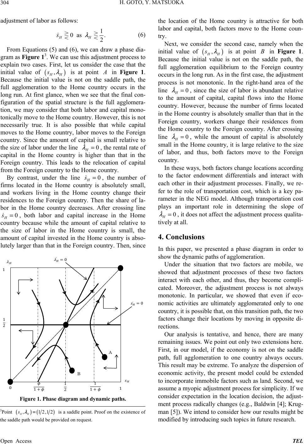 H. GOTO, Y. MATSUOKA 304 adjustment of labor as follows: 1 0 as . 2 HH s λ (6) From Equations (5) and (6), we can draw a phase dia- gram as Figure 13. We can use this adjustment process to explain two cases. First, let us consider the case that the initial value of ( is at point ) , HH s λ A in Figure 1. Because the initial value is not on the saddle path, the full agglomeration to the Home country occurs in the long run. At first glance, when we see that the final con- figuration of the spatial structure is the full agglomera- tion, we may consider that both labor and capital mono- tonically move to the Home country. However, this is not necessarily true. It is also possible that while capital moves to the Home country, labor moves to the Foreign country. Since the amount of capital is small relative to the size of labor under the line , the rental rate of capital in the Home country is higher than that in the Foreign country. This leads to the relocation of capital from the Foreign country to th e Home country. 0 H λ = By contrast, under the line , the number of firms located in the Home country is absolutely small, and workers living in the Home country change their residences to the Foreign country. Then the share of la- bor in the Home country decreases. After crossing line , both labor and capital increase in the Home country because while the amount of capital relative to the size of labor in the Home country is small, the amount of capital invested in the Home country is abso- lutely larger than that in the Foreign country. Th en, since 0 H s= 0 H s= 1 1 1 1 2 0 0 1 1 0 1 2 A B Figure 1. Phase diagram and dynamic paths. the location of the Home country is attractive for both labor and capital, both factors move to the Home coun- try. Next, we consider the second case, namely when the initial value of ( is at point in Figure 1. Because the initial value is not on the saddle path, the full agglomeration equilibrium to the Foreign country occurs in the long run. As in the first case, the adju stment process is not monotonic. In the right-hand area of the line , since the size of labor is abundant relative to the amount of capital, capital flows into the Home country. However, because the number of firms located in the Home country is absolutely smaller than that in the Foreign country, workers change their residences from the Home country to the Foreign country. After crossing line , while the amount of capital is absolutely small in the Home country, it is large relative to the size of labor, and thus, both factors move to the Foreign country. ) , HH s λ B 0 H λ = 0 H λ = In these ways, both factors change locations according to the factor endowment differentials and interact with each other in their adjustment processes. Finally, we re- fer to the role of transportation cost, which is a key pa- rameter in the NEG model. Although transportation cost plays an important role in determining the slope of , it does not affect the adjustment process qualita- tively at all. 0 H λ = 4. Conclusions In this paper, we presented a phase diagram in order to show the dynamic pat hs o f agglome ra t ion. Under the situation that two factors are mobile, we showed that adjustment processes of these two factors interact with each other, and thus, they become compli- cated. Moreover, the adjustment process is not always monotonic. In particular, we showed that even if eco- nomic activities are ultimately agglomerated only to one country, it is possible th at, on this tran sition path , the two factors change their locations by moving in opposite di- rections. Our analysis is tentative, and hence, there are many remaining issues. We point out only two extensions here. First, in our model, if the economy is not on the saddle path, full agglomeration to one country always occurs. This result may be extreme. To analyze the dispersion of economic activity, the present model could be extended to incorporate immobile factors such as land. Second, we assume a myopic adjustment process for simplicity. If we consider expectation in the location decision, the adjust- ment process radically changes (e.g., Baldwin [4]; Krug- man [5]). We intend to consider how our results might be modified by introducing such topics in future research. 3Point ()( ,12,1 HH s λ = ) 2 is a saddle point. Proof on the existence o f the saddle path would be provided on request. Open Access TEL  H. GOTO, Y. MATSUOKA Open Access TEL 305 5. Acknowledgements The authors thanks to No ritsugu Nakanishi, No buaki Ha- maguchi, Fumio Dei, Yasukazu Ichino, Takashi Shibata, Yang Xi, Chihiro Inaba, Miwa Nakai and participants of Rokko Forum at Kobe University, the 23th KMSG at Kushiro Public Un iversity of Economics and the seminar at Konan University. The second author was a JSPS re- search fellow and this work was financially supported by Grant-in-Aid for JSPS Fellows (No. 10J02314). This work was also supported in part by Grants for Excellent Graduate Schools, MEXT, Japan. Needless to say, any errors remaining in this paper are the responsibility of the authors. REFERENCES [1] R. E. Baldwin and A. J. Venables, “International Migra- tion, Capital Mobility and Transitional Dynamics,” Eco- nomica, Vol. 61, No. 243, 1994, pp. 285-300. http://dx.doi.org/10.2307/2554616 [2] P. Martin and C. A. Rogers, “Industrial Location and Public Infrastructure,” Journal of International Econom- ics, Vol. 39, No. 3-4, 1995, pp. 335-351. http://dx.doi.org/10.1016/0022-1996(95)01376-6 [3] A. K. Dixit and J. E. Stiglitz, “Monopolistic Competition and Optimum Product Diversity,” American Economic Review, Vol. 67, No. 3, 1977, pp. 297-308. [4] R. E. Baldwin, “Core-Periphery Model with Forward- Looking Expectations,” Regional Science and Urban Eco- nomics, Vol. 31, No. 1, 2001, pp. 21-49. http://dx.doi.org/10.1016/S0166-0462(00)00068-5 [5] P. Krugman, “History versus Expectations,” Quarterly Journal of Economics, Vol. 106, No. 2, 1991, pp. 651- 667. http://dx.doi.org/10.2307/2937950 |