Applying a Mathematical Model to the Performance of a Female Monofin Swimmer

doi:10.4236/am.2013.412228

Paper Menu >>

Journal Menu >>

Applied Mathematics, 2013, 4, 1673-1681

Published Online December 2013 (http://www.scirp.org/journal/am)

http://dx.doi.org/10.4236/am.2013.412228

Open Access AM

Applying a Mathematical Model to the Performance of a

Female Monofin Swimmer

Elisée Gouba1, Balira Ousmane Konfe2, Ousseynou Nakoulima3, Blaise Some1, Olivier Hue4

1Laboratoire LANIBIO, U.F.R. S.E.A., Université de Ouagadougou,

Ouagadougou, Burkina Faso

2Laboratoire LAIMA, Institut Africain d’Informatique, Libreville, Gabon

3Département de Mathématiques et Informatique, Université Antilles-Guyane,

Pointe-à-Pitre, France

4Laboratoire A.C.T.E.S., UPRES-EA 3596, U.F.R. S.T.A.P.S.-U.A.G.,

Faculté de Médecine, Pointe-à-Pitre, France

Email: [email protected], [email protected], [email protected], [email protected], [email protected]

Received March 6, 2013; revised April 6, 2013; accepted April 13, 2013

which permits unrestricted use, distribution, and reproduction in any medium, provided the original work is properly cited.

ABSTRACT

This study sought to determine the best method to quantify training based on heart rate data. It proposes a modification

of Banister’s original performance model to improve the accuracy of predicted performance. The new formulation in-

troduces a variable that accounts for changes in the subject’s initial performance as a result of the quantity of training.

The two systems models were applied to a well-trained female monofin swimmer over a 24-week training period. Each

model comprised a set of parameters unique to the individual and was estimated by fitting model-predicted performance

to measured performance. We used the Alienor method associated to Optimization-Preserving Operators to identify

these parameters. The quantification method based on training intensity zones gave a better estimation of predicted per-

formance in both models. Using the new model in sports in which performance is generally predicted (running, swim-

ming) will help us to define its real interest.

Keywords: Training Quantification; Banister’s Model

1. Introduction

In 1975, Banister et al. [1-4] proposed a systems model

to predict athletic performance. This model (and its ex-

tensions) is based on two antagonistic functions: the

positive function can be compared to a fitness impulse

resulting from the organism’s adaptation to training and

the negative function is similar to a fatiguing impulse.

Each function comprises a set of parameters that are in-

terpreted as the individual’s response profile, which can

be used for training prescription. Parameters include, for

example, time to recover performance and time to peak

performance after training completion.

Monofin swimming is a relatively new sport (recog-

nized by the IOC in 1986) that consists of propelling the

body at the water surface or underwater with an undula-

tion accentuated by the monofin [5,6]. Very high swim

velocities can thereby be reached (up to 14 km·h−1), and

this sport is attracting a growing number of enthusiasts.

Although a few studies have investigated the techniques

of monofin swimming [5,7-9], little is actually known

about fin swimmers and the parameters that contribute to

performance. In 2005, O. Hue et al. found that both an-

thropometric and physiological (aerobic and anaerobic

components) factors contributed to the performances of

French West Indian monofin swimmers. The finding that

both maximal oxygen uptake and the second ventilatory

threshold were significantly correlated with performance

[10], suggested that monofin swimming performance,

like running [11,12], swimming [13,14] and cycling [15],

could be extrapolated using Banister’s model. However,

this model had been criticized by several authors [16-19]

who reported that the practical interpretation of the posi-

tive and negative influences might be difficult. For ex-

ample, Taha and Thomas [19] criticized the models stem-

ming from Banister’s original model [13], stressing their

inability to accurately predict future performance, the

difference between the estimated time course of perform-

ance changes and experimental observations, and the fact

E. GOUBA ET AL.

1674

that most of these models were poorly corroborated by

physiological mechanisms.

In Banister’s model, performance is mathematically

related to the training load using any one of the three

basic methods of training quantification: a method using

the mathematical formula developed by Banister and

Hamilton [20], another using the three intensity zones

defined by the aerobic and anaerobic ventilatory thresh-

olds, and the last using five intensity zones. Although

several authors have used one or another method to

quantify training without providing justification (for ex-

ample [21-23] used the mathematical formula; and [12,

14,24] used the training quantification method with five

intensity zones), we cannot rule out the possibility that

using various training quantification methods may affect

the accuracy of performance prediction with Banister’s

model.

Our main objectives in this study of an internationally

ranked monofin swimmer were the followings: 1) to de-

termine the best method of quantifying training that pro-

vides a pertinent model over a 24-week training period

and for each time that performance is measured; and 2)

to propose a new model based on Banister’s original

model that would improve the accuracy of predicting

performance.

2. Methods

2.1. Subject

A 17-year-old female monofin swimmer, weighing 64 kg

for 164 cm, was recruited. The subject had previous

competitive swimming experience and at the time of the

study was among the top 15 monofin swimmers in the

Junior World ranking. The subject was fully informed of

the study conditions and gave written consent in accor-

dance with the regional ethics committee before partici-

pating.

2.2. The Progressive and Maximal Exercise Test

The ramp exercise test began with a 3-minute warm-up at

30 W, and the load was increased by 15 W every minute

until exhaustion. Pedaling speed remained constant at 70

rpm during the entire test.

Gas exchanges were measured during the first and

third repetitions using a breath-by-breath automated ex-

ercise metabolic system (Zan 680, Zan, Oberthulba, Ger-

many) and oxygen uptake was considered maximal (i.e.,

VO2max) if at least three of the following four criteria

were met:

1) a respiratory exchange ratio greater than 1.10,

2) attainment of age-predicted maximal heart rate

(HRmax) [210− (0.65 × age) ± 10%],

3) an increase in oxygen uptake (VO2) lower than 100

ml with the last increase in work rate, and

4) an inability to maintain the required pedaling fre-

quency (70 rpm) despite maximum effort and verbal en-

couragement. The heart rate at rest (HRrest) and the maxi-

mal aerobic power (MAP) were also determined. A 10-

lead electrocardiogram (12-lead ECG, Del Mar Deynolds,

Spacelabs, Healthcare Inc., UK) was used to monitor

heart rate continuously. The results are shown in Table

2.3. Ventilatory Threshold Determination

The ventilatory thresholds were visually determined ac-

cording to the method of Wasserman et al. [25,26],

which describes the inflection points in pulmonary ven-

tilation during incremental exercise. The ventilatory

thresholds (VTs) were identified when breakpoints oc-

curred in the VE/VO2 and VE/VCO2 curves. The first

ventilatory threshold (VT1) was identified by the point of

non-linear increase in VE and a clear increase in VE/VO2.

At the same time, VE/VCO2 remained constant or slightly

decreased. VT1 was also determined by the V-slope me-

thod of [27], which consisted of plotting VCO2 against

VO2 to identify a steep rise in VCO2 compared with the

rise in VO2 with increasing intensity. The second venti-

latory threshold (VT2), which corresponds to the respi-

ratory decompensation for metabolic acidosis, was iden-

tified by a second non-linear increase in VE and a second

clear increase in VE/VO2. At this point, VE rose more

rapidly than VCO2, leading to a rise in VCO2. Three ex-

perienced investigators independently deter- mined these

thresholds (Table 1).

2.4. Experimental Design

During a 24-week period, the subject continued her re-

gular training regime and recorded details of each train-

ing session. In addition, she completed performance tests

and fatigue questionnaires. The performance tests were

not conducted during periods of national or international

competition.

2.5. Fatigue Questionnaire

Before each performance test, the subject completed the

original version of the Profile of Mood States (POMS)

questionnaire developed in 1971 by McNair, Lorr &

Droppleman [28]. The subject used a 5-point scale (0 =

“not at all” to 4 = “extremely”) to respond to each item.

In the present study, only the responses to the fatigue

subset of the POMS were considered.

2.6. Performance Test

Performance tests over a distance of 700 m were made

every three weeks. During training sessions and per-

formance tests, the subject wore a heart rate monitor

Open Access AM

E. GOUBA ET AL.

Open Access AM

1675

Table 1. Physiological performance obtained for the subject.

VO2max VT1 VT2 MAP MAP (VT1)MAP (VT2)HRmax HR (VT1) HR (VT2)

ml·min−1·kg−1 % VO2max % VO2max watts watts watts bpm bpm bpm

45.5 61.5 82.1 232 151 202 194 155 181

VO2max, maximal oxygen uptake; VT1, ventilatory threshold; VT2, respiratory compensation threshold; MAP, maximal aerobic power (power attained at

VO2max); HRmax, maximal heart rate; MAP (VT1), maximal aerobic power at VT1; HR (VT1), heart rate corresponding to VT1.

(Polar S810i, Polar Electro, Kempele, Finland) that re-

corded heart rate every 5 s. The heart rate data for each

exercise bout was analyzed using Polar Precision soft-

ware.

3. Training Quantification

The exercise training intensity can be quantified using

several methods based on heart rate or lactate response,

the expression of intensity relative to maximum heart

rate or oxygen consumption, or the expression of inten-

sity relative to ventilation or the anaerobic threshold.

However, only the subset of methods generally used in

training-performance modeling were studied.

For each exercise session, training impulse (TRIMP)

was quantified three ways (Figure 1):

 With the mathematical formula developed by Banister

and Hamilton [20],

 Based on a repartition of heart rate into three zones of

intensity [29],

 Based on a breakdown of heart rate into five zones of

intensity [14].

3.1. Mathematical Formula

The mathematical formula is given by:



wtd k x

where is the exercise duration expressed in minutes,

is defined by:

exercise rest

max rest

RHR

xHR HR





and is related to the subject’s gender; in our study,

the subject was female, thus

1.67

0.86 e

k

Here rest

R indicates the lowest measure of heart rate

recorded when the subject is awake and max

R, the

highest recorded during incremental testing on a cycle

ergometer.

3.2. Training Quantification with Three Intensity

Zones

The three intensity zones were defined taking into ac-

count the HR corresponding to the ventilatory thresholds.

Zone 1 includes all HR below the first ventilatory

threshold, zone 2 contains the HR between the two

thresholds, and zone 3 includes all HR above the second

threshold.

The amount of training in each zone is equal to the ex-

ercise duration in minutes in this area, multiplied by the

physiological stress weighting factor for that intensity

zone (zone 1 → 1, zone 2 → 2, zone 3 →3). The training

impulse for each exercise bout was thus recorded as the

sum of the training impulse scores for each intensity

zone.

3.3. Training Quantification with Five Intensity

Zones

The five intensity zones were defined according to the

study of Wood et al. [12]. The physiological stress

weighting factor used for each training intensity zone has

been reported elsewhere [14].

Figure 1 present training loads performed by the sub-

ject during the course of the study; training loads are

quantified with the three methods of training quantifica-

tion

4. Modeling of the Response to Training

We used the model proposed by Banister et al. [13],

which considers the athlete as an open system with the

training impulse as the input and performance as the

output. This type of modeling models “cause” to “effect”

phenomena and usually leads directly to integral equa-

tions [30].

The time functions of performance and training

load







wt are mathematically related as





ptpp gt



(1)

where 0 is an additive term that depends on the initial

training status of the subject and * denotes the product of

convolution.

is a transfer function that depends on

time and is defined by



exp exp

gt kkt



 





 

 

(2)

where 1 and are gain terms and k2



and 2



are

time constants.

The definition of the convolution product leads to: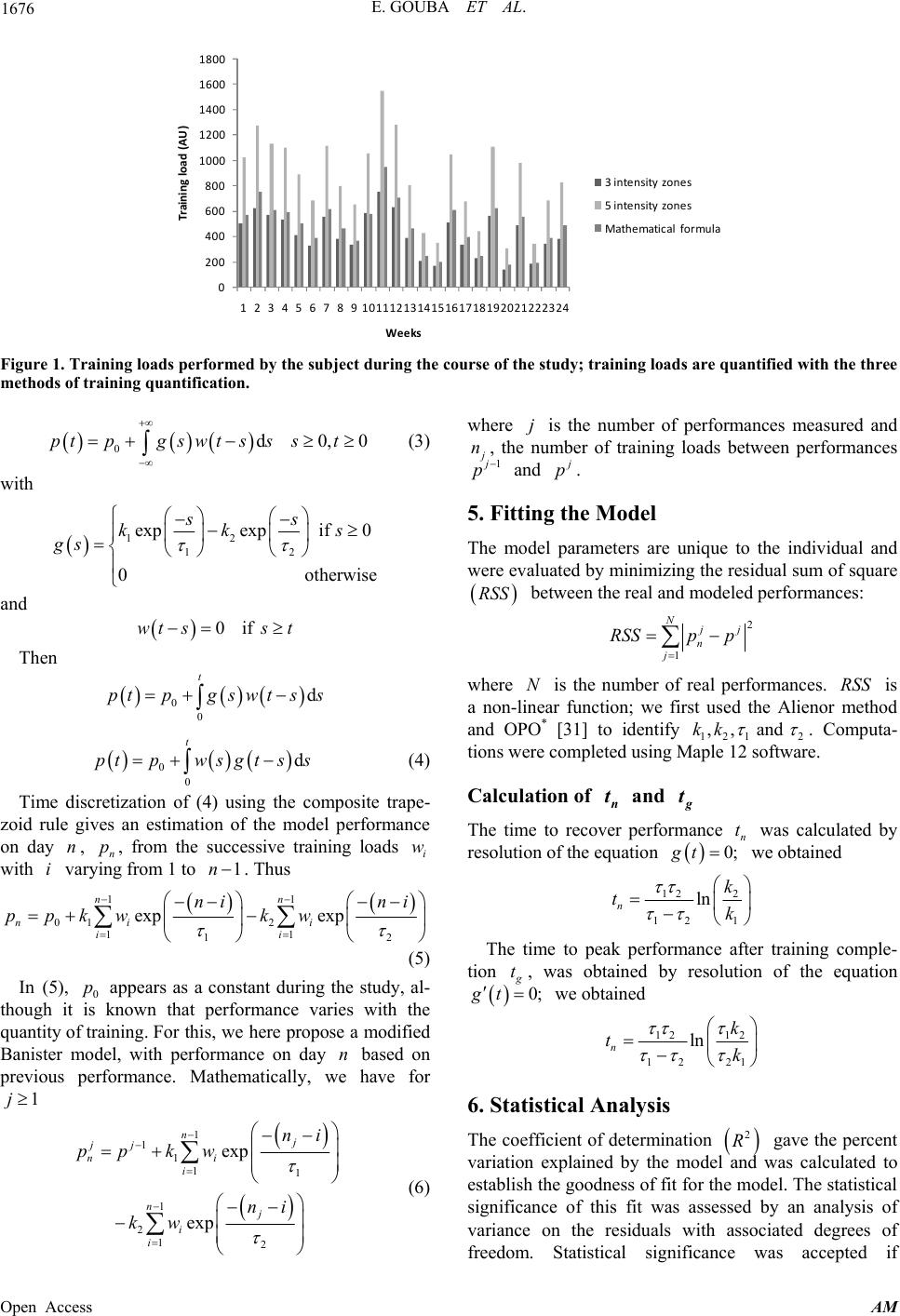

E. GOUBA ET AL.

1676

200

400

600

800

1000

1200

1400

1600

1800

123456789101112131415161718192021222324

Trainingload(AU)

Wee ks

3intensityzones

5intensityzones

Mathematic alformula

Figure 1. Training loads performe d by the subject during the course of the study; tr aining loads are quantified with the three

methods of training quantification.

 

0d0,ptpgswt ss st





 

0

(3)

with



expexpif 0



 





 

 



o

therwise

and



0ifwt sst 

Then

 

ptpgswt ss 



 

ptpwsgt ss 

 (4)

Time discretization of (4) using the composite trape-

zoid rule gives an estimation of the model performance

on day , n, from the successive training loads

with varying from 1 to

npi

i1n



. Thus







01 2

exp exp

ni i

ni ni

ppkw kw







  

 

 

 



(5)

In (5), 0 appears as a constant during the study, al-

though it is known that performance varies with the

quantity of training. For this, we here propose a modified

Banister model, with performance on day based on

previous performance. Mathematically, we have for

1j







exp

pp kw

















 















where is the number of performances measured and

n, the number of training loads between performances



and

5. Fitting the Model

The model parameters are unique to the individual and

were evaluated by minimizing the residual sum of square





RSS between the real and modeled performances:

RSSp p







where is the number of real performances. is

a non-linear function; we first used the Alienor method

and OPO* [31] to identify 121 2

NRSS

,, and kk



. Computa-

tions were completed using Maple 12 software.

Calculation of and

The time to recover performance n was calculated by

resolution of the equation we obtained



gt

12 2

12 1









The time to peak performance after training comple-

tion

t, was obtained by resolution of the equation





0;gt





we obtained

12 12

12 21



 







6. Statistical Analysis

The coefficient of determination gave the percent

variation explained by the model and was calculated to

establish the goodness of fit for the model. The statistical

significance of this fit was assessed by an analysis of

variance on the residuals with associated degrees of

freedom. Statistical significance was accepted if







(6)

Open Access AM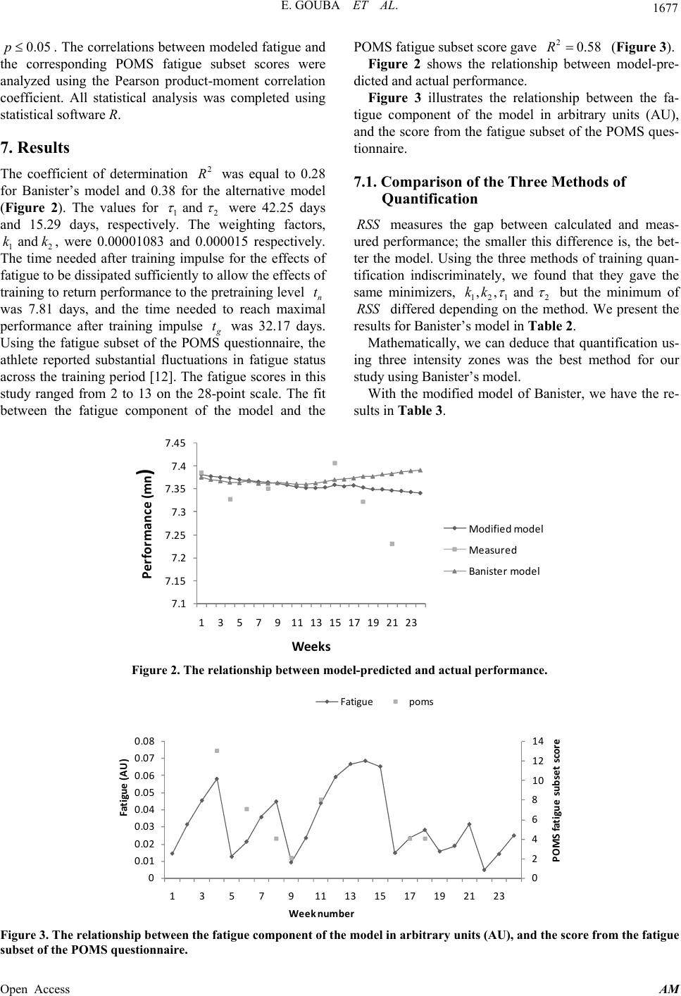

E. GOUBA ET AL. 1677

0.05p. The correlations between modeled fatigue and

the corresponding POMS fatigue subset scores were

analyzed using the Pearson product-moment correlation

coefficient. All statistical analysis was completed using

statistical software R.

7. Results

The coefficient of determination was equal to 0.28

for Banister’s model and 0.38 for the alternative model

(Figure 2). The values for 12

and



were 42.25 days

and 15.29 days, respectively. The weighting factors,

, were 0.00001083 and 0.000015 respectively.

The time needed after training impulse for the effects of

fatigue to be dissipated sufficiently to allow the effects of

training to return performance to the pretraining level n

was 7.81 days, and the time needed to reach maximal

performance after training impulse

and kk

t was 32.17 days.

Using the fatigue subset of the POMS questionnaire, the

athlete reported substantial fluctuations in fatigue status

across the training period [12]. The fatigue scores in this

study ranged from 2 to 13 on the 28-point scale. The fit

between the fatigue component of the model and the

POMS fatigue subset score gave (

Figure 3).

20.58R

Figure 2 shows the relationship between model-pre-

dicted and actual performance.

Figure 3 illustrates the relationship between the fa-

tigue component of the model in arbitrary units (AU),

and the score from the fatigue subset of the POMS ques-

tionnaire.

7.1. Comparison of the Three Methods of

Quantification

RSS measures the gap between calculated and meas-

ured performance; the smaller this difference is, the bet-

ter the model. Using the three methods of training quan-

tification indiscriminately, we found that they gave the

same minimizers, 121 2

,, and kk



but the minimum of

differed depending on the method. We present the

results for Banister’s model in Table 2.

RSS

Mathematically, we can deduce that quantification us-

ing three intensity zones was the best method for our

study using Banister’s model.

With the modified model of Banister, we have the re-

sults in Table 3.

7.1

7.15

7.2

7.25

7.3

7.35

7.4

7.45

1357911131517192123

Performance(mn

)

We eks

Modifiedmode l

Measured

Banistermodel

Figure 2. The relationship between mode l-pr edic ted and actual performance.

0.01

0.02

0.03

0.04

0.05

0.06

0.07

0.08

1357911131517192123

POMSfatiguesubsetscor e

Fat igue(AU)

Weeknumber

Fatigue poms

Figure 3. The relationship between the fatigue component of the model in arbitrary units (AU), and the score from the fatigue

subset of the POMS questionnaire.

Open Access AM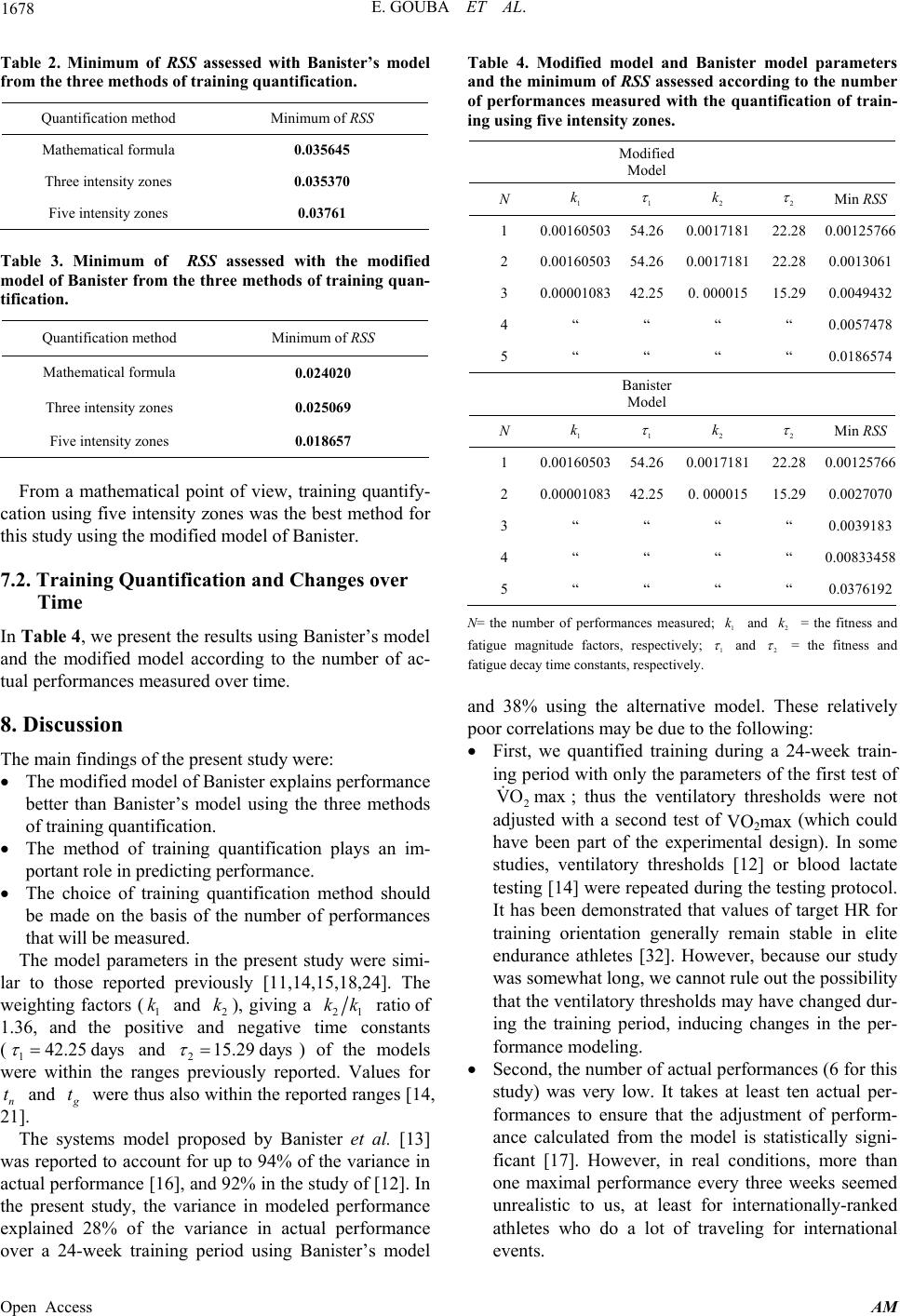

E. GOUBA ET AL.

1678

Table 2. Minimum of RSS assessed with Banister’s model

from the three methods of training quantification.

Quantification method Minimum of RSS

Mathematical formula 0.035645

Three intensity zones 0.035370

Five intensity zones 0.03761

Table 3. Minimum of RSS assessed with the modified

model of Banister from the three methods of training quan-

tification.

Quantification method Minimum of RSS

Mathematical formula 0.024020

Three intensity zones 0.025069

Five intensity zones 0.018657

From a mathematical point of view, training quantify-

cation using five intensity zones was the best method for

this study using the modified model of Banister.

7.2. Training Quantification and Changes over

Time

In Table 4 , we present the results using Banister’s model

and the modified model according to the number of ac-

tual performances measured over time.

8. Discussion

The main findings of the present study were:

 The modified model of Banister explains performance

better than Banister’s model using the three methods

of training quantification.

 The method of training quantification plays an im-

portant role in predicting performance.

 The choice of training quantification method should

be made on the basis of the number of performances

that will be measured.

The model parameters in the present study were simi-

lar to those reported previously [11,14,15,18,24]. The

weighting factors (1 and 2), giving a k k21

kk ratio of

1.36, and the positive and negative time constants

(142.25days



 and 215.29 days



) of the models

were within the ranges previously reported. Values for

n and t

t were thus also within the reported ranges [14,

21].

The systems model proposed by Banister et al. [13]

was reported to account for up to 94% of the variance in

actual performance [16], and 92% in the study of [12]. In

the present study, the variance in modeled performance

explained 28% of the variance in actual performance

over a 24-week training period using Banister’s model

Table 4. Modified model and Banister model parameters

and the minimum of RSS assessed according to the number

of performances measured with the quantification of train-

ing using five intensity zones.

Modified

Model

N 1

k 1



k 2



Min RSS

1 0.0016050354.26 0.0017181 22.28 0.00125766

2 0.0016050354.26 0.0017181 22.28 0.0013061

3 0.0000108342.25 0. 000015 15.29 0.0049432

4 “ “ “ “ 0.0057478

5 “ “ “ “ 0.0186574

Banister

Model

N 1

k 1



k 2



Min RSS

1 0.0016050354.26 0.0017181 22.28 0.00125766

2 0.0000108342.25 0. 000015 15.29 0.0027070

3 “ “ “ “ 0.0039183

4 “ “ “ “ 0.00833458

5 “ “ “ “ 0.0376192

N= the number of performances measured; and 2 = the fitness and

fatigue magnitude factors, respectively;



and 2



= the fitness and

fatigue decay time constants, respectively.

and 38% using the alternative model. These relatively

poor correlations may be due to the following:

 First, we quantified training during a 24-week train-

ing period with only the parameters of the first test of

VO max

; thus the ventilatory thresholds were not

adjusted with a second test of VO2max (which could

have been part of the experimental design). In some

studies, ventilatory thresholds [12] or blood lactate

testing [14] were repeated during the testing protocol.

It has been demonstrated that values of target HR for

training orientation generally remain stable in elite

endurance athletes [32]. However, because our study

was somewhat long, we cannot rule out the possibility

that the ventilatory thresholds may have changed dur-

ing the training period, inducing changes in the per-

formance modeling.

 Second, the number of actual performances (6 for this

study) was very low. It takes at least ten actual per-

formances to ensure that the adjustment of perform-

ance calculated from the model is statistically signi-

ficant [17]. However, in real conditions, more than

one maximal performance every three weeks seemed

unrealistic to us, at least for internationally-ranked

athletes who do a lot of traveling for international

events.

Open Access AM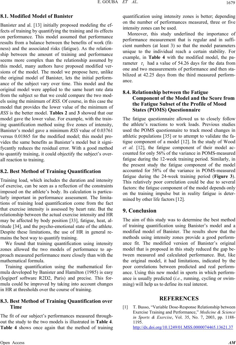

E. GOUBA ET AL. 1679

8.1. Modified Model of Banister

Banister and al. [13] initially proposed modeling the ef-

fects of training by quantifying the training and its effects

on performance. This model assumed that performance

results from a balance between the benefits of work (fit-

ness) and the associated risks (fatigue). As the relation-

ship between the amount of training and performance

seems more complex than the relationship assumed by

this model, many authors have proposed modified ver-

sions of the model. The model we propose here, unlike

the original model of Banister, lets the initial perform-

ance of the subject vary over time. This model and the

original model were applied to the same heart rate data

from the subject so that we could compare the two mod-

els using the minimum of RSS. Of course, in this case the

model that provides the lower value of the minimum of

RSS is the better model. Tables 2 and 3 showed that our

model gave the lower value. For example, with the train-

ing quantification method using five zones of intensity,

Banister’s model gave a minimum RSS value of 0.03761

versus 0.01865 for the modified model; this model pro-

vides the same benefits as Banister’s model but it signi-

fycantly reduces the residual error. With a good method

to quantify training, it could objectify the subject’s over-

all reaction to training.

8.2. Best Method of Training Quantification

Training load, which includes the duration and intensity

of exercise, can be seen as a reflection of the constraints

imposed on the athlete’s body. Its calculation is particu-

larly important in performance assessment. The limita-

tions of training load quantification come from the fact

that exercise intensity is assessed by heart rate. But the

relationship between the actual exercise intensity and HR

may be affected by body position [33], fatigue, heat, al-

titude [34], and the psycho-emotional state of the athlete.

Despite these limitations, the use of HR in general re-

mains the best way to quantify training.

We found that training quantification using intensity

zones allowed the two models of performance to ap-

proach measured performance more closely than with the

mathematical formula.

Training quantification using the mathematical for-

mula developed by Banister and Hamilton (1985) is easy

(logiperf software R2D2, Paris) and precise. This for-

mula could be improved by taking into account changes

in HR at thresholds over the course of training.

8.3. Best Method of Training Quantification over

Time

The fit of our subject’s performances measured through-

out the study to the two models is illustrated in Table 4.

Table 4 shows once again that the method of training

quantification using intensity zones is better; depending

on the number of performances measured, three or five

intensity zones can be used.

Moreover, this study underlined the importance of

performance measurement that is regular and in suffi-

cient numbers (at least 3) so that the model parameters

unique to the individual reach a certain stability. For

example, in Table 4 with the modified model, the pa-

rameter 1



had a value of 54.26 days for the data from

one and two measurements of performance and then sta-

bilized at 42.25 days from the third measured perform-

ance.

8.4. Relationship between the Fatigue

Component of the Model and the Score from

the Fatigue Subset of the Profile of Mood

States (POMS) Questionnaire

The fatigue questionnaire allowed us to closely follow

the athlete’s reactions to work loads. Previous studies

used the POMS questionnaire to track mood changes in

athletic populations [35] or to attempt to validate the fa-

tigue component of a model [12]. In the study of Wood

et al. [12], the fatigue component of their model ac-

counted for only 56% of the variance in POMS-measured

fatigue during the 12-week training period. Similarly, in

the present study the fatigue component of the model

accounted for 58% of the variance in POMS-measured

fatigue during the 24-week training period (Figure 3).

This relatively poor correlation could be due to several

factors: the fatigue component of the model depends only

on the training impulse but in reality fatigue is deter-

mined by other life factors [12].

9. Conclusion

The aim of this study was to determine the best method

of training quantification using Banister’s model and a

modified model of Banister. The results show that the

methods using intensity zones provide a good perform-

ance fit. The modified version of Banister’s original

model that is proposed in this study reduced the gap be-

tween measured and calculated performance. But, like

the original model, it had limitations, indicated by the

poor correlations between predicted and real perform-

ance. Using this new model in sports in which perform-

ance is usually predicted (i.e., running, cycling or swim-

ming) will help us to define its real interest.

REFERENCES

[1] T. Busso, “Variable Dose-Response Relationship between

Exercise Training and Performance,” Medicine & Science

in Sports & Exercise, Vol. 35, No. 7, 2003, pp. 1188-

1195.

http://dx.doi.org/10.1249/01.MSS.0000074465.13621.37

Open Access AM

E. GOUBA ET AL.

1680

[2] T. Busso, C. Denis, R. Bonnefoy, A. Geyssant and J. R.

Lacour, “Modeling of Adaptations to Physical Training

by Using a Recursive Least Squares Algorithm,” Journal

of Applied Physiology, Vol. 82, No. 5, 1997, pp. 1685-

1693.

[3] T. Busso, C. Denis, H. Benoît, R. Bonnefoy, L. Feasson

and J. R. Lacour, “Effects of Training Frequency on the

Dynamics of the Performance Response to a Single Train-

ing Bout,” Journal of Applied Physiology, Vol. 92, No. 2,

2002, pp. 572-580.

[4] T. W. Calvert, E. W. Banister, M. V. Savage and T. Bach,

“Systems Model of the Effect of Training on Physical

Performance,” IEEE Transactions on Systems, Man, and

Cybernetics, Part B, Vol. 6, No. 2, 1976, pp. 94-102.

[5] L. Baly, D. Favier and A. Durey, “Finswimming Techni-

cal Description by 3D Kinematic Study,” Archives of

Physiology and Biochemistry, Vol.109, No. 1, 2001, p.

67.

[6] R. H. Sanders, J. M. Cappaert and R. K. Devlin, “Waves

Characteristics of Butterfly Swimming,” Journal of Bio-

mechanics, Vol. 28, No. 1, 1995, pp. 9-16.

http://dx.doi.org/10.1016/0021-9290(95)80002-6

[7] J. Gautier, L. Baly, P. R. Zanone and B. Watier, “A Ki-

nematic Study of Finswimming at Surface,” Journal of

Sports Science and Medicine, Vol. 3, No. 2, 2004, pp. 91-

95.

[8] M. A. Luersen, R. Leriche, D. Lemosse and O. A. Lemaî-

tre, “A Computationally Efficient Approach to Swimming

Monofin Optimization,” Structural and Multidisciplinary

Optimization, Vol. 31, No. 6, 2006, pp. 488-496.

http://dx.doi.org/10.1007/s00158-006-0001-6

[9] R. Marek and B. Grazyna, “Searching for Criteria in

Evaluating the Monofin Swimming Trun from the Per-

spective of Coaching and Improvement Technique,”

Journal of Sports Science and Medicine, Vol. 7, No. 1,

2008, pp. 67-77.

[10] O. Hue, O. Galy, S. Blonc and C. Hertogh, “Anthropom-

etrical and Physiological Determinants of Performance in

French West Indian Monofin Swimmers: A First Ap-

proach,” International Journal of Sports Medicine, Vol.

27, No. 8, 2006, pp. 605-609.

http://dx.doi.org/10.1055/s-2005-865856

[11] R. H. Morton, J. R. Fitz-Clarke and E. W. Banister, “Mo-

deling Human Performance in Running,” Journal of Ap-

plied Physiology, Vol. 69, No. 3, 1990, pp. 1171-1177.

[12] R. E. Wood, S. Hayter, D. Rowbottom and I. Stewart,

“Applying a Mathematical Model to Training Adaptation

in a Distance Runner,” European Journal of Applied Phy-

siology, Vol. 94, No. 3, 2005, pp. 310-316.

http://dx.doi.org/10.1007/s00421-005-1319-2

[13] E. W. Banister, T. W. Calvert, M. V. Savage and T. M.

Batch, “A Systems Model of Training for Athletic Per-

formance,” Journal of Science and Medicine in Sport, Vol.

7, No. 3, 1975, pp. 57-61.

[14] I. Mujika, T. Busso, L. Lacoste, F. Barale, A. Geyssant

and J. C. Chatard, “Modeled Response to Training and

Taper in Competitive Swimmers,” Medicine & Scienc e in

Sports & Exercise, Vol. 28, No. 2, 1996, pp. 251-258.

http://dx.doi.org/10.1097/00005768-199602000-00015

[15] T. Busso, C. Carosso and J. R. Lacour, “Adequacy of a

Systems Structure in the Modeling of Training Effects on

Performance,” European Journal of Applied Physiology,

Vol. 61, No. 1-2, 1991, pp. 48-54.

http://dx.doi.org/10.1007/BF00236693

[16] T. Busso, K. Hakkinen, A. Pakarinen, C. Carasso, J. R.

Lacour, P. V. Komi and H. Kauhanen, “A Systems Model

of Training Responses and Its Relationships to Hormonal

Responses in Elite Weight-Lifters,” European Journal of

Applied Physiology, Vol. 61, No. 1-2, 1990, pp. 48-54.

http://dx.doi.org/10.1007/BF00236693

[17] J. C. Chatard, T. Busso, F. Barale and L. Lacoste,

“Quantification et Modélisation de l’entraînement en Na-

tation,”STAPS: Sciences et Techniques des Activités Phy-

siques et Sportives, Vol. 33, 1994, pp. 7-17.

[18] P. Hellard, M. Avalos, L. Lacoste, F. Barale, J. C. Cha-

tard and G. P. Millet, “Assessing the Limitations of the

Banister Model in Monotoring Training,” Journal of

Sports Sciences, Vol. 24, No. 5, 2006, pp. 509-520.

http://dx.doi.org/10.1080/02640410500244697

[19] T. Taha and S. G. Thomas, “Systems Modeling of the Re-

lationship between Training and Performance,” Sports

Medicine, Vol. 33, No. 14, 2003, pp. 1061-1073.

http://dx.doi.org/10.2165/00007256-200333140-00003

[20] E. W. Banister and C. L. Hamilton, “Variations in Iron

Status with Fatigue Modeled from Training in Female

Distance Runners,” European Journal of Applied Physi-

ology, Vol. 54, No. 1, 1985, pp. 16-23.

http://dx.doi.org/10.1007/BF00426292

[21] E. W. Banister, J. B. Carter and P. C. Zarkadas, “Training

Theory and Taper: Validation on Triathlon Athletes,” Eu-

ropean Journal of Applied Physiology, Vol. 79, No. 2,

1999, pp. 182-191.

http://dx.doi.org/10.1007/s004210050493

[22] S. Le Bris, B. Ledermann, N. Topin, P. Messner-Pellenc

and D. Le Gallais, “A Systems Model of Training for Pa-

tients in Phase 2 Cardiac Rehabilitation,” International

Journal of Cardiology, Vol. 109, No. 2, 2006, pp. 257-

263. http://dx.doi.org/10.1016/j.ijcard.2005.06.029

[23] G. P. Millet, A. Groslambert, B. Barbier, J. D. Rouillon

and R. B. Candau, “Modelling the Relationships between

Training, Anxiety, and Fatigue in Elite Athletes,” Inter-

national Journal of Sports Medicine, Vol. 26, No. 6, 2005,

pp. 492-498. http://dx.doi.org/10.1055/s-2004-821137

[24] L. Thomas, I. Mujika and T. Busso, “A Model Study of

Optimal Training Reduction during Pre-Event Taper in

Elite Swimmers,” Journal of Sports Science, Vol. 26, No.

6, 2008, pp. 643-652.

http://dx.doi.org/10.1080/02640410701716782

[25] K. Wasserman and M. B. Mcllroy, “Detecting the Thresh-

old of Anaerobic Metabolism in Cardiac Patient during

Exercise,” American Journal of Cardiology, Vol. 14, No.

6, 1964, pp. 844-852.

http://dx.doi.org/10.1016/0002-9149(64)90012-8

[26] K. Wasserman, B. J. Whipp, S. Koyal and W. L. Beaver,

“Anaerobic Threshold and Respiratory Gas Exchange

during Exercise,” Journal of Applied Physiology, Vol. 35,

No. 2, 1973, pp. 236-243.

[27] W. L. Beaver, K. Wasserman and B. J. Whipp, “A New

Open Access AM

E. GOUBA ET AL.

Open Access AM

1681

Method for Detecting Anaerobic Threshold by Gas Ex-

change,” Journal of Applied Physiology, Vol. 60, No. 6,

1986, pp. 2020-2027.

[28] D. M. McNair, M. Lorr and L. F. Droppleman, “Profile of

Mood States Manual,” Educational and Industrial Testing

Service, San Diego, 1971.

[29] S. K. Seiler and ØG. Kjerland, “Quantifying Training

Intensity Distribution in Elite Endurance Athletes: Is There

Evidence for an ‘Optimal’ Distribution?” Scandinavian

Journal of Medicine & Science in Sports, Vol. 16, No. 1,

2006, pp. 49-56.

http://dx.doi.org/10.1111/j.1600-0838.2004.00418.x

[30] Y. Cherruault, “Modèles et Méthodes Mathématiques

Pour les Sciences du Vivant,” Presses Universitaires de

France, 1998.

[31] B. O. Konfé, Y. Cherruault, B. Somé and T. Bennouala,

“Alienor Method Applied to Operational Research,” Ky-

bernetes, Vol. 34, No. 7-8, 2005, pp. 1211-1222.

http://dx.doi.org/10.1108/03684920510605984

[32] A. Lucia, J. Hoyos, M. Pérez and J. L. Chicharro, “Heart

Rate and Performance Parameters in Elite Cyclists: A

Longitudinal Study,” Medicine & Science in Sports &

Exercise, Vol. 32, No. 10, 2000, pp. 1777-1782.

http://dx.doi.org/10.1097/00005768-200010000-00018

[33] R. Perini, C. Orizio, S. Milesi, L. Biancardi, G. Baselli

and A. Veicsteinas, “Body Position Affects the Power

Spectrum of Heart Rate Variability during Dynamic Ex-

ercise,” European Journal of Applied Physiology, Vol. 66,

No. 3, 1993, pp. 207-213.

http://dx.doi.org/10.1007/BF00235095

[34] J. R. Lacour, “Biologie de L’Exercice Musculaire,” Mas-

son, Paris, 1992.

[35] I. M. Cockrill, A. M. Nevill and N. Lyons, “Modelling

Mood States in Athletic Performance,” Journal of Sports

Science, Vol. 9, No. 2, 1991, pp. 205-212.

http://dx.doi.org/10.1080/02640419108729881