Apply of Explicit Finite Element in Seismic Ground Motion Computation

doi:10.4236/jamp.2013.16003

Paper Menu >>

Journal Menu >>

Journal of Applied Mathematics and Physics, 2013, 1, 11-14

Published Online November 2013 (http://www.scirp.org/journal/jamp)

http://dx.doi.org/10.4236/jamp.2013.16003

Open Access JAMP

Apply of Explicit Finite Element in Seismic Ground

Motion Computation*

Yuzhu Bai, Xiwei Xu

Active Tectonics and Volcano Lab, Key Lab of China Earthquake Administration, Beijing, China

Email: [email protected]

Received August 2013

ABSTRACT

In this paper, we will u se the explicit finite element to compute ground motion due to Tangshan earthquake. The expli-

cit finite-element method uses one integration point and an hourglass control scheme. We implement the coarse-grain

method in a structured finite-element mesh straightforw ardly. At the same time, we also apply the coarse -grain method

to a widely used, slightly unstructured finite-element mesh, where unstructured finite elements are only used in the ver-

tical velocity transition zones. By the finite-element methods, we can compute the ground velocity with some distance

to the seismogenic fault in Tangshan earthquake. Through the computation, we can find the main character of ground

motion for the s t r i ke sl ip eart hq uake event s and the hi gh freque nc y vibrat ion moti on of groun d motion.

Keywords: Finite-Element Method; Fault; Ground Motion; Tangshan Earthquake

1. Introduction

In earthquake research, we often mainly apply the finite-

difference and finite-element method to calculate the

ground motion due to the movement of the seismic faults.

The finite-element method, one of the most popular me-

thods in the engineering science, is increasingly used in

earthquake computation (see [1-3]) and earthquake dy-

namic rupture propagatios (see [4,5]). With the help of

irregular elements of different size, geometry, and order

of approximations, the finite-element is efficient to mod-

el complic ate d geomet rica l boundary condi tions at pres ent .

The explicit finite-element method with second-order

elements and one-point integration is widely used. This

method combines the flexibility of the finite-element

method and the efficiency of finite-difference method.

As its efficiency and versatility, this method has been

widely implemented and applied to transient analyses in

engineering and seismology. Here, we refer to this par-

ticular implementation as the explicit finite-element me-

thod.

The following algorithm for th e explicit finite-element

method is easy. Usually, it uses for-node quadrilateral

elements in two dimensions and eight-node hexahedral

elements in three dimensions and applies one integration

point and an hourglass control scheme. Because of the

computational costs and the numerical noise resulting

from the ad hoc mass lumping necessary to generate a

diagonal mass matrix (see [6] ), higher-order elements are

rarely used in researching transient problems. But one-

point integration provides tremendous computational

benefits in dynamic simulations. Comparing with the full

integration, one-point integration has a 3/4 reduction in

computational time in two dimensions and 7/8 reduction

in three dimensions. At the same time, one-point integra-

tion also provides the efficient way to simulate n onlinear

material response (see [7]).

In fact, the one-point integratio n in the elements has its

own drawback which is a mesh instability known as

hourglassing. But the hourglass modes can be eliminated

by well-developed hourglass control schemes (see [8]).

Kosloff and Frazier [9] had showed that a one-point in-

tegration implementation coupled with a stiffness hour-

glass control scheme can produce a more accurate flex-

ural response than fully integrated elements. So in this

article, we will apply the finite-element with one-point

integration developed by Ma [10] to compute the ground

velocity of some location s varyin g with time in the T an g-

shan earthquake.

2. Explicit Finite-Element Algorithm and

Tectonic Background

2.1. Explicit F in it e-Element Algorithm

Here we will use the explicit finite element develop ed by

Ma [10], so we will introduce his method in a simple

*Subsidized by “Discern and evaluation of earthquake risk zone

(2012BAK15B01)”.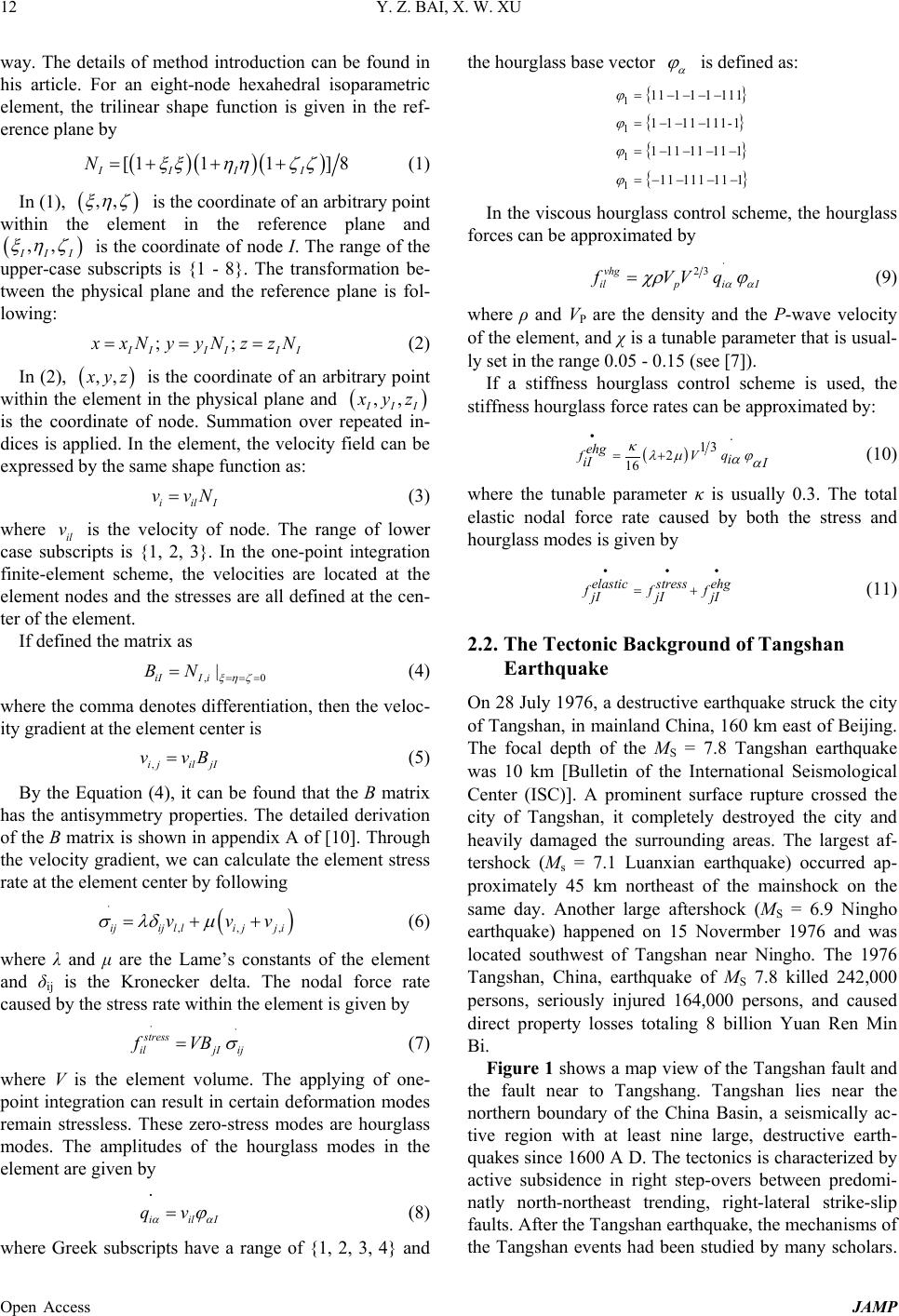

Y. Z. BAI, X. W. XU

Open Access JAMP

way. The details of method introduction can be found in

his article. For an eight-node hexahedral isoparametric

element, the trilinear shape function is given in the ref-

erence plane by

( )()()

[111 ]8

I III

ξξηηζ ζ

=+++

(1)

In (1),

( )

ξηζ

is the coordinate of an arbitrary point

within the element in the reference plane and

( )

III

ξηζ

is the coordinate of node I. The range of the

upper-case subscripts is {1 - 8}. The transformation be-

tween the physical plane and the reference plane is fol-

lowing:

;;

IIII II

xxNyyN zzN== =

(2)

In (2),

( )

,,xyz

is the coordinate of an arbitrary point

within the element in the physical plane and

( )

III

xyz

is the coordinate of node. Summation over repeated in-

dices is applied. In the element, the velocity field can be

expressed by the same shape function as:

iil I

v vN=

(3)

where

is the velocity of node. The range of lower

case subscripts is {1, 2, 3}. In the one-point integration

finite-element scheme, the velocities are located at the

element nodes and the stresses are all defined at the cen-

ter of the element.

If defined the m a trix as

iIIi

ξηζ

= = =

(4)

where the comma denotes differentiation, then the veloc-

ity gradient at the element center is

,i jiljI

v vB=

(5)

By the Equation (4), it can be found that the B matrix

has the antisymmetry properties. The detailed derivation

of the B matrix is shown in appendix A of [10]. Through

the velocity gradient, we can calculate the element stress

rate at the element center by following

( )

, ,,ijijl lijj i

v vv

σ λδµ

⋅

= ++

(6)

where λ and μ are the Lame’s constants of the element

and δij is the Kronecker delta. The nodal force rate

caused by the stress rate within the element is given by

stress

iljI ij

f VB

⋅⋅

(7 )

where V is the element volume. The applying of one-

point integration can result in certain deformation modes

remain stressless. These zero-stress modes are hourglass

modes. The amplitudes of the hourglass modes in the

element are given by

iilI

αα

⋅

(8)

where Greek subscripts have a range of {1, 2, 3, 4} and

the hourglass base vector

is defined as:

{ }

11111111

1 1 11 111-1

11111111

11 111 11 1

= −−−−

=−− −

= −−−−

=−− −−

In the viscous hourglass control scheme, the hourglass

forces can be approximated by

23vhg

ilpi I

fVV q

αα

χρ ϕ

⋅

(9)

where ρ and VP are the density and the P-wave velocity

of the element, and χ is a tunable parameter that is usual-

ly set in the range 0.05 - 0.15 (see [7]).

If a stiffness hourglass control scheme is used, the

stiffness hourglass force rates can be approximated by:

( )

ehg

f Vq

iI I

κλµ ϕ

αα

⋅

= +



(1 0 )

where the tunable parameter κ is usually 0.3. The total

elastic nodal force rate caused by both the stress and

hourglass modes is given by

ehg

elastic stress

f ff

jIjI jI

= +





(11)

2.2. The Tectonic Background of Tangshan

Earthquake

On 28 July 1976, a destructive earthquake struck the city

of Tangshan, in mainland China, 160 km east of Beijing.

The focal depth of the MS = 7.8 Tangshan earthquake

was 10 km [Bulletin of the International Seismological

Center (ISC)]. A prominent surface rupture crossed the

city of Tangshan, it completely destroyed the city and

heavily damaged the surrounding areas. The largest af-

tershock (Ms = 7.1 Luanxian earthquake) occurred ap-

proximately 45 km northeast of the mainshock on the

same day. Another large aftershock (MS = 6.9 Ningho

earthquake) happened on 15 Novermber 1976 and was

located southwest of Tangshan near Ningho. The 1976

Tangshan, China, earthquake of MS 7.8 killed 242,000

persons, seriously injured 164,000 persons, and caused

direct property losses totaling 8 billion Yuan Ren Min

Bi.

Figure 1 shows a map view of the Tangshan fault and

the fault near to Tangshang. Tangshan lies near the

northern boundary of the China Basin, a seismically ac-

tive region with at least nine large, destructive earth-

quakes since 1600 A D. The tectonics is characterized by

active subsidence in right step-overs between predomi-

natly north-northeast trending, right-lateral strike-slip

faults. After the Tangshan earthquake, the mechanisms of

the Tangshan events had been studied by many scholars.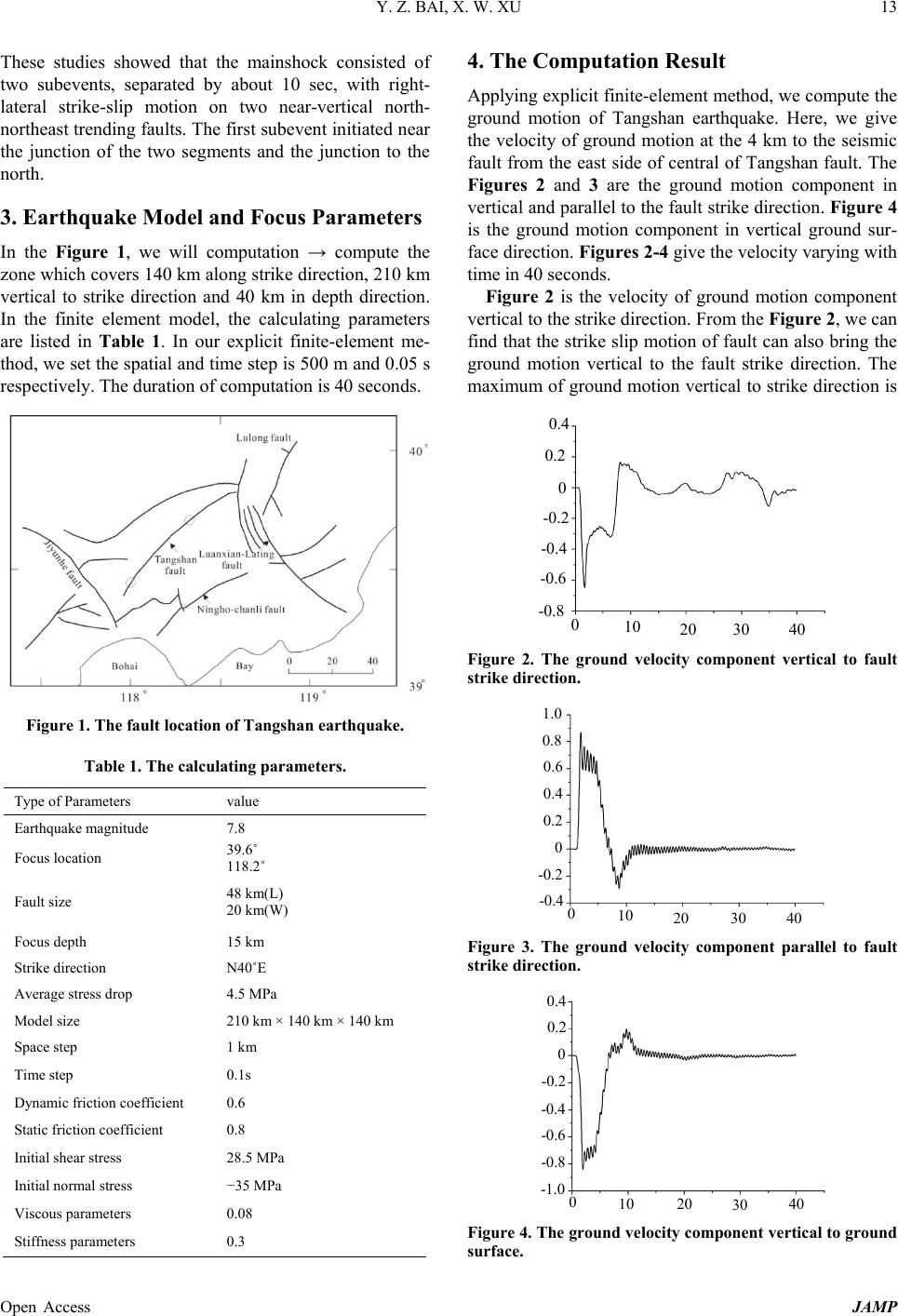

Y. Z. BAI, X. W. XU

Open Access JAMP

These studies showed that the mainshock consisted of

two subevents, separated by about 10 sec, with right-

lateral strike-slip motion on two near-vertical north-

northeast trending faults. The first subev ent initiated near

the junction of the two segments and the junction to the

north.

3. Earthquake Model and Focus Parameters

In the Figure 1, we will computation → compute the

zone which covers 140 km along strike direction, 210 km

vertical to strike direction and 40 km in depth direction.

In the finite element model, the calculating parameters

are listed in Table 1. In our explicit finite-element me-

thod, we set the spatial and time step is 500 m and 0.05 s

respectively. The duration of computation is 40 seconds.

Figure 1. The fault location of Tangshan earthquake.

Table 1. The calculating parameters.

Type of Parameters value

Earthquake magnitude 7.8

Focus location 39.6˚

118.2˚

Fault size 48 k m( L)

20 km( W )

Focus depth 15 km

Strike direction N40˚E

Average stress drop 4.5 MPa

Model size 210 km × 140 km × 140 km

Space step 1 km

Time step 0.1s

Dynamic friction coefficient 0.6

Static friction coefficient 0.8

Initial shear stress 28.5 MPa

Initial normal stress −35 MPa

Viscous parameters 0.08

Stiffness parameters 0.3

4. The Computation Result

Applying explicit finite-element method, we compute the

ground motion of Tangshan earthquake. Here, we give

the velocity of ground motion at the 4 km to the seismic

fault from the east side of central of Tangshan fault. The

Figures 2 and 3 are the ground motion component in

vertical and parallel to the fault strik e direction. Figure 4

is the ground motion component in vertical ground sur-

face direction. Figures 2-4 give the velocity varying with

time in 40 seconds.

Figure 2 is the velocity of ground motion component

vertical to the strike direction. From the Figure 2, w e can

find that the strike slip motion of fault can also bring the

ground motion vertical to the fault strike direction. The

maximum of ground motion vertical to strike direction is

-0.8

-0.6

-0.4

-0.2

0.2

0.4

Figure 2. The ground velocity component vertical to fault

strike direction.

0.4

0.2

-0.4

-0.2

0.6

0.8

1.0

Figure 3. The ground velocity component parallel to fault

strike direction.

-0.6

-0.4

0.4

-0.2

-0.8

-1.0

0.2

Figure 4. The ground velocity component vertical to ground

surface.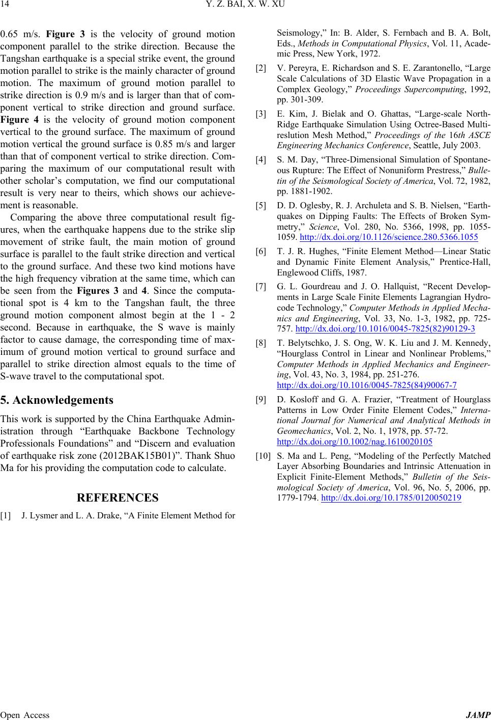

Y. Z. BAI, X. W. XU

Open Access JAMP

0.65 m/s. Figure 3 is the velocity of ground motion

component parallel to the strike direction. Because the

Tangshan earthquake is a special strike event, the ground

motion parallel to strike is the mainly character of ground

motion. The maximum of ground motion parallel to

strike direction is 0.9 m/s and is larger than that of com-

ponent vertical to strike direction and ground surface.

Figure 4 is the velocity of ground motion component

vertical to the ground surface. The maximum of ground

motion vertical the ground surface is 0.85 m/s and larg er

than that of component vertical to strike direction. Com-

paring the maximum of our computational result with

other scholar’s computation, we find our computational

result is very near to theirs, which shows our achieve-

ment is reasonable.

Comparing the above three computational result fig-

ures, when the earthquake happens due to the strike slip

movement of strike fault, the main motion of ground

surface is parallel to the fault strike direction and vertical

to the ground surface. And these two kind motions have

the high frequency vibration at the same time, which can

be seen from the Figures 3 and 4. Since the computa-

tional spot is 4 km to the Tangshan fault, the three

ground motion component almost begin at the 1 - 2

second. Because in earthquake, the S wave is mainly

factor to cause damage, the corresponding time of max-

imum of ground motion vertical to ground surface and

parallel to strike direction almost equals to the time of

S-wave travel to the computational spot.

5. Acknowledgements

This work is supported by the China Earthquake Admin-

istration through “Earthquake Backbone Technology

Professionals Foundations” and “Discern and evaluation

of earthquake risk zone (2012BAK15B01)”. Thank Shuo

Ma for his providing the computation code to calculate.

REFERENCES

[1] J. Lysmer and L. A. Drake, “A Finite E le ment M ethod for

Seismology,” In: B. Alder, S. Fernbach and B. A. Bolt,

Eds., Methods in Computational Physics, Vol. 11, Acade-

mic Press, New York, 1972.

[2] V. Pereyra, E. Richardson and S. E. Zarantonello, “Large

Scale Calculations of 3D Elastic Wave Propagation in a

Complex Geology,” Proceedings Supercomputing, 1992,

pp. 301-309.

[3] E. Kim, J. Bielak and O. Ghattas, “Large-scale North-

Ridge Earthquake Simulation Using Octree-Based Multi-

reslution Mesh Method,” Proceedings of the 16th ASCE

Engineering Mechanics Conference, Seattle, July 2003.

[4] S. M. Day, “Three-Dimensional Simulation of Spontane-

ous Rupture: The Effect of Nonuniform Prestress,” Bulle-

tin of t he Sei smological Society of America, Vol. 72, 1982,

pp. 1881-1902.

[5] D. D. Oglesby, R. J. Archuleta and S. B. Nielsen, “Earth-

quakes on Dipping Faults: The Effects of Broken Sym-

metry ,” Science, Vol. 280, No. 5366, 1998, pp. 1055-

1059. http://dx.doi.org/10.1126/science.280.5366.1055

[6] T. J. R. Hughes, “Finite Element Method—Linear Static

and Dynamic Finite Element Analysis,” Prentice-Hall,

Englewood Cliffs, 1987.

[7] G. L. Gourdreau and J. O. Hallquist, “Recent Develop-

ments in Large Scale Finite Elements Lagrangian Hydro-

code Technology,” Computer Methods in Applied Mecha-

nics and Engineering, Vol. 33, No. 1-3, 1982, pp. 725-

757. http://dx.doi.org/10.1016/0045-7825(82)90129-3

[8] T. Belytschko, J. S. Ong, W. K. Liu and J. M. Kennedy,

“Hourglass Control in Linear and Nonlinear Problems,”

Computer Methods in Applied Mechanics and Engineer-

ing, Vol. 43, No. 3, 1984, pp. 251-276.

http://dx.doi.org/10.1016/0045-7825(84)90067-7

[9] D. Kosloff and G. A. Frazier, “Treatment of Hourglass

Patterns in Low Order Finite Element Codes,” Interna-

tional Journal for Numerical and Analytical Methods in

Geomechanics, Vol. 2, No. 1, 1978, pp. 57-72.

http://dx.doi.org/10.1002/nag.1610020105

[10] S. Ma and L. Peng, “Modeling of the Perfectly Matched

Layer Absorbing Boundaries and Intrinsic Attenuation in

Explicit Finite-Element Methods,” Bulletin of the Seis-

mological Society of America, Vol. 96, No. 5, 2006, pp.

1779-1794. http://dx.doi.org/10.1785/0120050219