Saddle Point Solution for System with Parameter Uncertainties

doi:10.4236/apm.2013.38092

Paper Menu >>

Journal Menu >>

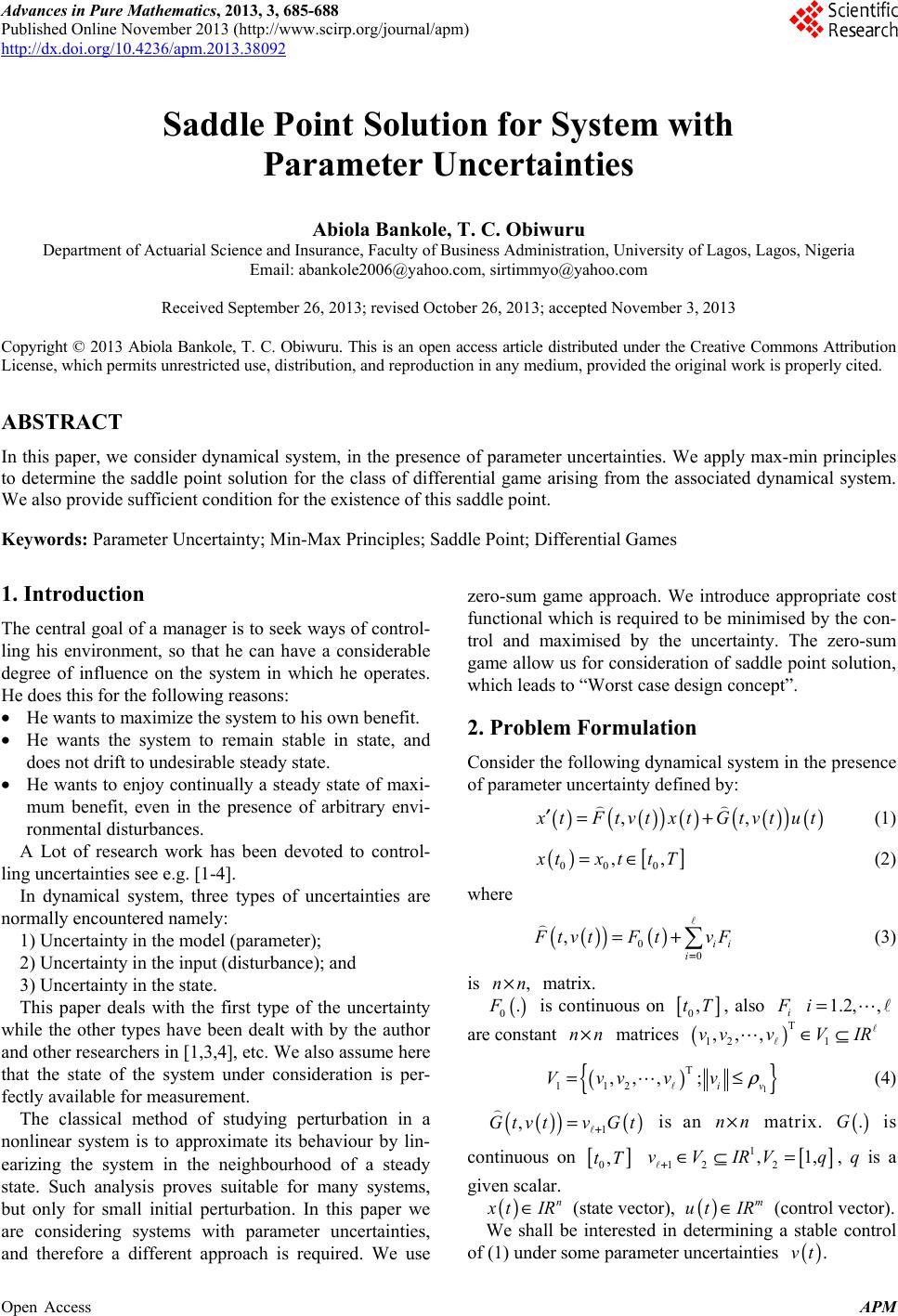Advances in Pure Mathematics, 2013, 3, 685-688

Published Online November 2013 (http://www.scirp.org/journal/apm)

http://dx.doi.org/10.4236/apm.2013.38092

Open Access APM

Saddle Point Solution for System with

Parameter Uncertainties

Abiola Bankole, T. C. Obiwuru

Department of Ac tuarial Scienc e and Insurance, Faculty of Business Administration, University of Lagos, Lagos, Nigeria

Email: [email protected], [email protected]

Received September 26, 2013; revised October 26, 2013; accepted November 3, 2013

License, which permits unrestricted use, distribution, and reproduction in any medium, provided the original work is properly cited.

ABSTRACT

In this paper, we consider dynamical system, in the presence of parameter uncertainties. We apply max-min principles

to determine the saddle point solution for the class of differential game arising from the associated dynamical system.

We also provide sufficient condition for the existence of this saddle point.

Keywords: Parameter Uncertainty; Min-Max Principles; Saddle Point; Differential Games

1. Introduction

The central goal of a manager is to seek ways of control-

ling his environment, so that he can have a considerable

degree of influence on the system in which he operates.

He does this for the following reasons:

• He wants to maximize the system to his own benefit.

• He wants the system to remain stable in state, and

does not dri ft to und esi rable steady state.

• He wants to enjoy continually a steady state of maxi-

mum benefit, even in the presence of arbitrary envi-

ronmental disturbances.

A Lot of research work has been devoted to control-

ling uncertainties see e.g . [1 -4].

In dynamical system, three types of uncertainties are

normally encountered na mely:

1) Uncertainty in the model (parameter);

2) Uncertainty in the input (disturbance); and

3) Uncertainty in the state.

This paper deals with the first type of the uncertainty

while the other types have been dealt with by the author

and other researchers in [1,3,4], etc. We also assume here

that the state of the system under consideration is per-

fectly available for measurement.

The classical method of studying perturbation in a

nonlinear system is to approximate its behaviour by lin-

earizing the system in the neighbourhood of a steady

state. Such analysis proves suitable for many systems,

but only for small initial perturbation. In this paper we

are considering systems with parameter uncertainties,

and therefore a different approach is required. We use

zero-sum game approach. We introduce appropriate cost

functional which is required to be minimised by the con-

trol and maximised by the uncertainty. The zero-sum

game allow us for consideration of saddle point solution,

which leads to “Worst case design concept”.

2. Problem Formulation

Consider the following dynamical system in the presence

of parameter uncertainty defined by:

() ()

()

() ()

()

tF tvtxtGtvtut

′=+



(1)

()

[

]

00 0

txttT=∈ (2)

where

()

,ii

tvtF tvF







(3)

is matrix.

,nn×

()

0.F is continuous on

[

]

0,tT, also i

1.2, ,i=



are constant matrices

nn×

()

12 1

,,,vvvV IR∈⊆



T

()

{

}

112

,,, ;iv

Vvvvv



≤

(4)

()

,Gtvtv Gt

=



is an matrix. is nn×

()

continuous on

[

]

0,tT

[

]

12 2

,1,vVIRV q

+∈⊆ =

, q is a

given scalar.

()

tIR∈ (state vector), (control vector).

()

ut IR∈

We shall be interested in determining a stable control

of (1) under some parameter uncertainties

()

.vt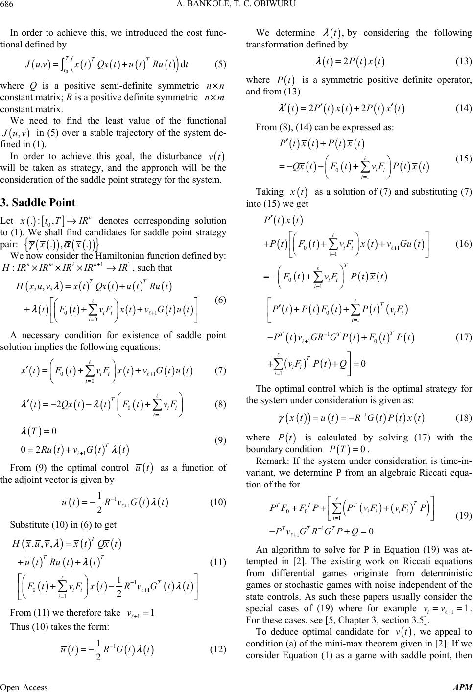

A. BANKOLE, T. C. OBIWURU

686

In order to achieve this, we introduced the cost func-

tional defined by

( )()()()()

()

TTT

uvx tQx tutRu tt=+

 (5)

where Q is a positive semi-definite symmetric

constant matrix; R is a positive definite symmetric

constant matrix.

nn×

nm×

We need to find the least value of the functional

(

)

uv in (5) over a stable trajectory of the system de-

fined in (1).

In order to achieve this goal, the disturbance

will be taken as strategy, and the approach will be the

consideration of the saddle point strategy for the system.

()

3. Saddle Point

Let

()

[

]

.: ,n

tT IR→ denotes corresponding solution

to (1). We shall find candidates for saddle point strategy

pair:

()

{

}

., .xx

γα

We now consider the Ham i ltonia n fu nction defined by:

:nmn 1

IRIRIR IRIR

××× →

, such that

()()() ()()

()()()() ()

,,,TT

Hxuvxt QxtutRut

tFt vFxtvGtut





+++













(6)

A necessary condition for existence of saddle point

solution implies the following equations:

()()()() ()

0ii

tFtvFxtvGtut



′=+ +









 (7)

()() ()()

tQxttFtvF

λλ



′=− −+







 (8)

()

()() ()

02 T

Ru tvG tt



(9)

From (9) the optimal control

()

ut as a function of

the adjoint vector is given by

() () ()

utRv Gtt

−

=−  (10)

Substitute (10) in (6) to get

()() ()

()()()

() ()() ()

,,,

HxuvxtQxt

ut Rutt

tvFxtRvGtt

−





+−



















(11)

From (11) we therefore take

11v+=



Thus (10) takes the form:

()() ()

utRGt t

−

=− (12)

We determine by considering the following

transformation define d by

()

()()()

2tPtxt

= (13)

where is a symmetric positive definite operator,

and from (13)

()

()() ()()()

22tPtxt Ptxt

′′ ′

=+ (14)

From (8), (14) can be expressed as:

() ()() ()

()()() ()

01ii

Ptxt Ptxt

Qx tFtvFPt x t

′+



=− −+







 (15)

Taking

()

t as a solution of (7) and substituting (7)

into (15) we get

() ()

() ()() ()

()() ()

Ptxt

PtF tvFxtvGut

FtvF Ptxt

−

′







+++















=− +









(16)

()() ()()

()

()()() ()

()

P tPtFtPtvF

PtvGRGPt FtPt

vFP tQ

−

′++





−+



++=









(17)

The optimal control which is the optimal strategy for

the system under consideration is given as:

()

()()() ()

tut RGtPtxt

−

==− (18)

where is calculated by solving (17) with the

boundary condition .

()

0PT =

Remark: If the system under consideration is time-in-

variant, we determine P from an algebraic Riccati equa-

tion of the for

()( )

()

00 1

TT T

ii ii

TTT

PFFPPvFvFP

PvGRGP Q

−





++ +









−+=





(19)

An algorithm to solve for P in Equation (19) was at-

tempted in [2]. The existing work on Riccati equations

from differential games originate from deterministic

games or stochastic games with noise independent of the

state controls. As such these papers usually consider the

special cases of (19) where for example .

For these cases, see [5, Chapter 3, section 3.5]. 11



To deduce optimal candidate for , we appeal to

condition (a) of the mini-max theorem given in [2]. If we

consider Equation (1) as a game with saddle point, then

()

Open Access APM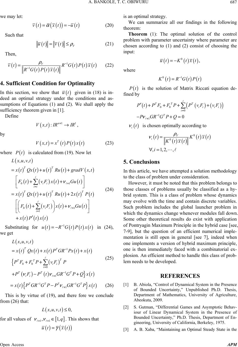

A. BANKOLE, T. C. OBIWURU 687

we may let:

() ()

()

vtxt ut

==− (20)

Such that

() ()

ut vt

=≤ (21)

Then,

() ()() () ()() ()

vt RGtPtxt

RGtPtxt

−

= (22)

4. Sufficient Condition for Optimality

In this section, we show that

()

ut given in (18) is in-

deed an optimal strategy under the conditions and as-

sumptions of Equations (1) and (2). We shall apply the

sufficiency theorem given in [1].

Define

()

,: n

Vxt IRIR

+→,

()()() ()

VxtxtPtxt= (23)

where is calculated from (19). Now let

()

()()()()()

()

() ()

()()()()() ()

()

() ()

()() ()

,,,

TT T

Lxuvt

tQxtutRutgradVx t

FtvFxt Gut

tQxt utRutxtPt

FtvF xtGut

xtP txt

=++







=++













′

















(24)

Substituting for in (24),

we get

()()()()

ut RGtPtxt

−

=−

()

()() ()() ()

{

()

}

()

00 0

,,,

TT ii

TT T

Lxuvt

tQxt xtPGRPxtxt

PFF PvFP

PFPtGRGPQxt

νν

−

=+ +

+− +





(25)

()

{

}

()

TTT T

tPGRGPP GRGPxt

−−

=−

 (26)

This is by virtue of (19), and there fore we conclude

from (26) that:

()

,,,0,Lxuvt≤

for all values of

[

]

,1,q

νν

∈

 . This shows that

() ()

()

ut xt

is an optimal strategy.

We can summarize all our findings in the following

theorem:

Theorem (1): The optimal solution of the control

problem with parameter uncertainty where parameter are

chosen according to (1) and (2) consist of choosing the

input:

()() ()

0,utK txt=−

where

()() ()

tRGtPt

−

()

Pt is the solution of Matrix Riccati equation de-

fined by

()

()( )

()

00 0

TT T

ii ii

PtPFFPP vFvF

PGRGPQ

−

′++++

−+=





()

is chosen optimally according to

() () () () ()

,1,2,,

itK

Ktxt

∀= 

txt

5. Conclusions

In this article, we have attempted a solution methodology

to the class of problem under consideration.

However, it must be noted that this problem belongs to

those classes of problems usually be classified as a hy-

brid system. This is a class of problem whose dynamics

may evolve with the time and contain discrete variables.

Such problem includes the global launcher problem in

which the dynamics change whenever modules f all down .

Some other theoretical results do exist with application

of Pontryagin Maximum Principle in the hybrid case [see,

7-9], but the question of an efficient numerical imple-

mentation is still open in general [see 7], indeed when

one implements a version of hybrid maximum principle,

one is then immediately faced with a combinatorial ex-

plosion. An efficient method to handle this class of prob-

lem needs to be developed.

REFERENCES

[1] B. Abiola, “Control of Dynamical System in the Presence

of Bounded Uncertainty,” Unpublished Ph.D. Thesis,

Department of Mathematics, University of Agriculture,

Abeokuta, 2009.

[2] S. Gutman, “Differential Games and Asymptotic Behav-

iour of Linear Dynamical System in the Presence of

Bounded Uncertainty,” Ph.D. Thesis, Department of En-

gineering, University of California, Berkeley, 1975.

[3] A. B. Xaba, “Maintaining an Optimal Steady State in the

Open Access APM

A. BANKOLE, T. C. OBIWURU

Open Access APM

688

Presence of Persistence Disturbance,” Ph.D. Dissertation,

University of Arizona, Tucson, 1984.

[4] C. S. Lee and Leitmann, “Uncertain Dynamical Systems:

An Application to River Pollution Control,” Modelling

and Management, Resources Uncertainty Workshop, Ea st-

West Centre, Honolulu, 1985.

[5] H. Kwakernaak, “Linear Optimal Control Systems,” Wi-

ley-Interscience, New York, 1972.

[6] F. H. Clarke, “Optimization of Nonsmooth Analysis, Ca-

nadian Mathematical Society Series of Monographs and

Advanced Texts,” John Wiley & Sons, Inc., New York,

1983.

[7] R. F. Hart, S. P. Sethi and R. G. Vickson, “A Survey of

the Maximum Principle for Optimal Control Problems

with State Constraints,” SIAM Review, Vol. 37, No. 2,

1995, pp. 181-218. http://dx.doi.org/10.1137/1037043

[8] T. Haberkorn and E. Trélat, “Convergence Results for

Smooth Regularizations of Hy brid Nonlinear Optimal Con-

trol Problems,” SIAM Journal on Control Optimization,

Vol. 49, No. 4, 2011, pp. 1498-1522.

http://dx.doi.org/10.1137/100809209

[9] R. Vinter, “Optimal Control, Systems & Control: Foun-

dations & Applications,” Birkauser, Boston, 2000.